Robotics-inspired methods to enhance protein design

(1)

HAL Id: tel-01591457

https://hal.laas.fr/tel-01591457

Submitted on 21 Sep 2017

HAL is a multi-disciplinary open access archive for the deposit and dissemination of sci-entific research documents, whether they are pub-lished or not. The documents may come from teaching and research institutions in France or abroad, or from public or private research centers.

L’archive ouverte pluridisciplinaire HAL, est destinée au dépôt et à la diffusion de documents scientifiques de niveau recherche, publiés ou non, émanant des établissements d’enseignement et de recherche français ou étrangers, des laboratoires publics ou privés.

Robotics-inspired methods to enhance protein design

Laurent Denarie

To cite this version:

Laurent Denarie. Robotics-inspired methods to enhance protein design. Robotics [cs.RO]. INP DE TOULOUSE, 2017. English. �tel-01591457�

(2)

THÈSE

En vue de l’obtention du

DOCTORAT DE L’UNIVERSITÉ FÉDÉRALE

TOULOUSE MIDI-PYRÉNÉES

Délivré par :

l’Institut National Polytechnique de Toulouse (INP Toulouse)

Présentée et soutenue le 12/04/2017 par :

Laurent DENARIE

Robotics-inspired methods to enhance protein design

JURY

Rachid ALAMI Directeur de Recherche Président du Jury

Charles ROBERT Directeur de Recherche Rapporteur

Marilena VENDITTELLI Professeur Assistant Rapporteur

Stéphane REDON Chargé de Recherche Examinateur

Thierry SIMÉON Directeur de Recherche Directeur de thèse Juan CORTÉS Directeur de Recherche Co-directeur de thèse

École doctorale et spécialité :

MITT : Domaine STIC : Intelligence Artificielle

Unité de Recherche :

Laboratoire d’analyse et d’architecture des systèmes

Directeur(s) de Thèse :

Thierry SIMÉON et Juan CORTÉS

Rapporteurs :

(3)

(4)

i

Acknowledgments

Cette thèse est le fruit de plus de trois années de travail au cours desquelles j’ai pu bénéficier de nombreux soutiens. Cette section est dédiée à toutes celles et ceux qui ont contribué, de près ou de loin, à la réussite de ce projet.

Je remercie chaleureusement mon directeur et mon co-directeur de thèse, Thierry SIMÉON et Juan CORTÉS. Thierry a été présent dans les moments im-portants et a toujours su donner des conseils avisés. Juan a été un soutien sans faille durant ces trois années de travail. Toujours présent lors de mes nombreuses sollicitations, il a su guider mes pas sur le chemin difficile du doctorat, faisant sans cesse naître de nouvelles idées.

Je remercie Charles ROBERT et Marilena VENDITTELLI, tout deux rappor-teurs de mon manuscrit de thèse, pour m’avoir fait l’honneur d’accepter d’évaluer mon travail et de me faire bénéficier de leur expertise.

Je remercie également Stéphane REDON pour avoir accepté de siéger en tant qu’examinateur au sein mon jury.

Je remercie Rachid ALAMI pour m’avoir accueilli au sein de son équipe au LAAS-CNRS et pour avoir accepté de siéger en tant qu’examinateur au sein mon jury.

Je souhaite également remercier mes collègues qui ont contribué d’une manière ou d’une autre à ce travail et plus particulièrement :

• Marc VAISSET pour ses conseils toujours avisés, sa disponibilité, et son effi-cacité à résoudre les bugs. Son professionnalisme et à sa bonne humeur font de lui un collègue hors pair.

• Kevin MOLLOY pour ses nombreux conseils et pour sa convivialité. Mon travail n’aurait pas été aussi abouti sans son aide précieuse. Nos chemins se recroiseront.

• Didier DEVAURS pour sa disponibilité.

• Ellon PAIVA MENDES pour son aide précieuse en LA_TEX.

• Alejandro ESTAÑA, Amélie BAROZET, et Maud JUSOT pour m’avoir sup-porté pendant tout ce temps, pour avoir mis le nez dans mon code, et pour avoir contribué à la bonne humeur de l’équipe.

Je remercie Stéphane CAMBON pour m’avoir mis en contact avec Rachid ALAMI et pour m’avoir permis de commencer cette aventure.

Ces remerciements seraient incomplets sans y inclure toutes les personnes qui ont indirectement permis de mener ce projet à bien.

Je remercie tout d’abord ma compagne, Anne BRUNO, qui a été le socle sur lequel j’ai pu me reposer tout au long de mon doctorat. Elle a su me supporter dans les moments difficiles et a été une source de motivation. Elle a également été une source d’inspiration, et le sera encore.

(5)

ii

Je remercie mes parents qui ont su faire de moi ce que je suis aujourd’hui. Je remercie Pierrick, Elena, Artur, et Aïva pour les moments de détente aussi bien sur les fauteuils de la cafétériat que dans les baudriers.

Je remercie Laurent, Laura, Jessica, et David pour les bouffées d’air pur données au cours de ce marathon.

Je remercie Nicolas, Harmish, Renaud, Alexandre, Marco, Michelangelo, Gré-goire, Ellon (à nouveau), Benjamin, Wuwei, Jules, César, Amandine, Sandra, Sarah, Arthur, Lancelot, Christophe, Clara, Etienne, Raphaël, et Mamoun pour la bonne humeur apportée au sein du laboratoire, et souvent en dehors également, que ce soit autour d’un café, d’une bière ou d’une table de pingpong.

(6)

Glossary

6R Six-revolute. Used to indicate that a serial manipulator has six revolution joints. This corresponds to the shortest full instantaneous mobility of the end frame relatively to the base frame of the manipulator.

C_α α-carbon of an amino acid to which is attached the side-chain. ecDHFR Escherichia coli DHFR

CFN Cost Function Network

CPD Computational Protein Design DEE Dead-End Elimination

DHF 7,8-dihydrofolate EST Expansive-Spaces Trees GA Genetic Algorithms MC Monte Carlo

MD Molecular Dynamics

mDH modified Denavit-Hartenberg NMR Nuclear Magnetic Resonance PCA Principal Component Analysis

PDB Protein Data Bank - Worldwide database of protein structures accessible online (http://www.rcsb.org/)

PRM Probabilistic Roadmap

RMSD Root Mean Square Deviation RRT Rapidly-exploring Random Tree

SDAP Simultaneous Design And Path-planning

SDAP Simultaneously Design And Path-planning algorithm T-RRT Transition-based RRT

(11)

viii Contents

Voronoi regions A Voronoi region is associated to every vertex in a search space. It denotes the region of space that is closer to that vertex than to other vertices.

(12)

Introduction

Proteins probably are the molecules the most representative of life. They are present is all living cells, and they are involved in most of the biological processes. They fulfill a wide range of functions, such as catalysis, regulation, signaling, transport, storage, and structural functions. In addition to their primary importance in biol-ogy, proteins are also key items in other domains. They are pharmaceutical targets of drugs, their catalytic properties are exploited in biotechnology, and they are used as components of nano-devices in the rising field of bionanotechnology. Although the properties of natural proteins can be directly exploited in all these domains, the ability to create new proteins with improved properties or new functions is of major interest.

Proteins are complex molecules. These chains of amino acids are flexible struc-tures whose shape, determined by the amino acid sequence, is strongly related to the function. Thus, designing a protein with the desired function consists in find-ing an amino acid sequence yieldfind-ing the suitable structure. Considerfind-ing the current knowledge on proteins and the experimental tools which are available today, achiev-ing such a task is plausible. Yet, the number of possible sequences to test is so large, and the experimental cost of synthesizing and testing a single sequence is so high that it is necessary to resort to computational methods. Those methods, called Computational Protein Design (CPD) methods, cannot replace experimental test-ing. Nevertheless, they allow to guide the design process toward a narrow number of candidate sequences on which experimental ressources will be focused.

CPD methods have been developed for more than a decade and they have al-ready permitted the creation of a few new proteins. Current CPD methods rely on a common approach that consist in finding, from a goal 3D scaffold, amino acid sequences that will fold into that scaffold. This problem is translated to an opti-mization problem. The main challenge lies in the nature and high dimensionality of the space to explore. This hybrid space has a discrete component, that corresponds to the set of all the possible amino acid sequences, and a continuous component, that corresponds to the possible configurations of the protein. Therefore, solving the optimization problem requires the use of algorithms allowing to efficiently explore such large spaces. In that regard, algorithms coming from the robotic community have demonstrated very promising abilities.

This thesis presents contributions toward the goal of solving such type of op-timization problems in hybrid spaces. These contributions are both at a sampling level, to improve the efficiency of algorithms designed for exploring the conforma-tional space of proteins (e.g. the space of protein’s spatial arrangement), and also at the algorithmic level. The first chapter of this thesis provides some background on protein modeling and design. It first introduces the basics of protein systems modeling. Then, it gives an overview of state of the art algorithms used to explore the conformational landscape of proteins. Finally, the protein design problem, is

(13)

2 Contents

introduced together with the current approaches to solve it and the limitations they suffer.

The second chapter presents a framework to enhance the sampling of proteins conformational space using stochastic algorithms such as Monte Carlo methods. By using a mechanistic representation of proteins, involving segmentation into small fragments of three amino acid residues, this framework simplifies the conception of new local backbone perturbation methods. This framework is demonstrated by the construction of several Monte Carlo move classes, all operating on a common protein representation. These sampling techniques are then compared on two different protein systems.

The third chapter presents a comparison of four conformational space explo-ration algorithms. Two existing ones, the T-RRT algorithm and a simple MC simulation, and two new ones, adapted from the robot motion planning algorithm EST. An empirical comparative analysis shows how T-RRT is superior in its abil-ity to quickly discover transition path between basins in the energy landscape of a protein.

Finally, the fourth chapter deals with an optimization problem that combines design and motion planning. The goal is to find the design (among a large set of possibilities) that optimizes the motion of the system between two given configu-rations. For this, the optimal path for all possible designs has to be searched. An algorithm to solve this problem is proposed and demonstrated on a simple academic system. Then, the application of the approach for designing a protein (or protein fragment) to perform a desired motion is investigated and discussed.

Contributions of the thesis

The work presented in this thesis is part of the development of a robotics-inspired algorithm library for structural biology. The previous developments performed by LAAS-CNRS in this context have shown the promising potential of these techniques for the study of protein flexibility [Cortés 2005]. A practical example of applica-tion of these methods to the simulaapplica-tion of protein-ligand unbinding is available at http://moma.laas.fr/ [Devaurs 2013a].

In the ProtiCAD project founded by the Agence nationale de la recherche (ANR), the goal was to adapt robotics-inspired algorithms to be part of a CPD procedure taking protein flexibility into account. In this context, my scientific con-tributions are on multiple levels:

• Enhancement of local conformation sampling: We extended the sampling methods previously published in [Cortés 2012] by implementing a new move class (the Hinge move class) and by performing a comparative analysis of the different local move class involving the tripeptide decomposition model. This work led to the submission of a journal paper at JCTC [Denarie 2017]. • Study of fast conformational landscape exploration methods: We implemented

(14)

Contents 3

the transition test already used in the T-RRT costspace exploration technique [Jaillet 2010].

• Adaptation of robotics-inspired algorithm for CPD: We formalized a new op-timization problem inspired from CPD and proposed an algorithm, called SDAP, to solve it. This work has been published at the Workshop on the Algorithmic Foundations of Robotics 2016 [Denarie 2016].

(15)

(16)

Chapter 1 Scientific Context

Contents

1.1 Proteins sequence and structure . . . . 5

1.1.1 Amino acids, peptides, and proteins . . . 5

1.1.2 Sequence-function relationship . . . 8

1.2 Protein modeling . . . . 8

1.2.1 Cartesian coordinates . . . 9

1.2.2 Internal coordinates . . . 9

1.2.3 Dimensionality reduction . . . 10

1.2.4 Coarse grained models . . . 11

1.3 Energy landscape . . . . 12

1.3.1 Physical theory . . . 12

1.3.2 Energy functions . . . 13

1.4 Computational methods for the exploration of protein con-formations . . . . 14

1.4.1 Molecular dynamics . . . 15

1.4.2 Monte Carlo methods . . . 16

1.4.3 Robotics-inspired algorithms for the exploration of the confor-mational space . . . 17

1.5 Computational Protein Design . . . . 21

1.5.1 The CPD problem . . . 22

1.5.2 The search space . . . 23

1.5.3 Current methods for CPD . . . 24

1.5.4 CPD challenges . . . 25

Recent advances in computational structural biology are in a large part due to the improvement of simulation algorithms combined with the evolution of protein modeling. This chapter presents the basics of protein constitution and working in order to understand the high complexity of those systems. Some focus is made on the different modeling methods that were developed over the years before intro-ducing the notion of energy landscape. Then, an overview of the methods used to characterize or to explore the energy landscape is performed to finally present the computational protein design problem and explain the current approaches and the future challenges.

(17)

6 Chapter 1. Scientific Context

1.1 Proteins sequence and structure

1.1.1 Amino acids, peptides, and proteins

Amino acids are the building blocks of proteins. They contain an amine group (−NH₂), a carboxylic acid group (−COOH), and a connecting carbon atom, called

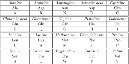
α-carbon (C_α) , to which is attached a group of atoms called the side-chain as shown in Figure 1.1. The side-chain, denoted by R, determines the physico-chemical properties of each amino acid type. In nature, there are twenty different types of side-chains corresponding to twenty different types of amino acids. They are listed in table 1.1 with their one-letter and three-letter codes.

H₂N C_α R C OH O

Figure 1.1: Representation of an amino acid with its α-carbon (black), its amine group (blue), its carboxylic acid group (red), and its side chain (green).

Alanine Arginine Asparagine Aspartic acid Cysteine

Ala Arg Asn Asp Cys

A R N D C

Glutamic acid Glutamine Glycine Histidine Isoleucine

Glu Gln Gly His Ile

E Q G H I

Leucine Lysine Methionine Phenylalanine Proline

Leu Lys Met Phe Pro

L K M F P

Serine Threonine Tryptophan Tyrosine Valine

Ser Thr Trp Tyr Val

S T W Y V

Table 1.1: Amino acids list with their 3-letter and 1-letter codes.

The amine group of an amino acid can react with the carboxylic acid group of another amino acid to form a peptide bond (see Figure 1.2). This process, called condensation, joins two amino acids together forming a dipeptide. When involved in a peptide or a polypeptide, amino acids are referred as residues. The amine group of the first amino acid and the carboxylic acid group from the second amino acid are preserved, so the condensation reaction can be repeated again and again to build a longer chain of amino acid residues. Such a chain is called a peptide,

(18)

1.1. Proteins sequence and structure 7 H₂N C_α R C OH O + C_α H₂N R C OH O H₂N C_α R C O N H C_α R C OH O + H₂O

Figure 1.2: Formation of a peptide bond (red).

H₂N C_α R C O N H C_α R C O N H C_α R C O N H C_α R C O OH

Figure 1.3: Backbone of a 4 residue peptide (in red). The N-terminus is on the left side of the figure while the C-terminus is on the right side of the figure.

or a polypeptide. A continuous thread of covalent bonds can be followed from the first to the last amino acid successively joining an amino nitrogen to an α-carbon, an α-carbon to a carboxylic carbon, and a carboxylic carbon to the next amino nitrogen. This chain of atom is called the backbone. The first residue’s amine group is called the N-terminus, and the last residue’s carboxylic acid group is called the C-terminus. A representation of the backbone can be seen in Figure 1.3. The sequence of a peptide/polypeptide is described by the list of the amino acids in the chain from the N-terminus to the C-terminus. It is usually represented using the one-letter code of the amino acids.

Peptides/polypeptides are flexible molecules and may take different spatial ar-rangements. Such an arrangement is called a conformation. Because of that, atoms from a residue may have interactions not only with adjacent residues’ atoms and external atoms (from the solvent, a ligand, or another peptide) but also with atoms of other residues far away in the polypeptide’s sequence. These interactions can form recognizable local structures, which are relatively stable and which are used

(19)

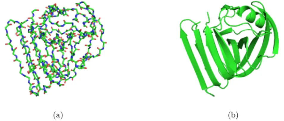
(a) (b)

Figure 1.4: Representation of a conformation of a protein (xylanase) using (a) stick representation (b) cartoon representation. In both figures, only the backbone is represented. The cartoon representation uses some symbol to recognize usual secondary structures like α-helices or β-sheet.

to simplify the representation of a molecule conformation. Figure 1.4 shows an example of such a representation.

Protein is the term employed to describe a polypeptide or a conglomerate of polypeptides bound together that have a biological function.

1.1.2 Sequence-function relationship

Proteins cover a very wide range of biological functions. They can be enzymes that catalyze some chemical reactions. They can be part of the process of signal transmission (this is the case of insulin for instance) or work as receptors of such a signal. They can bind other molecules called ligands, or they can dock on other macromolecules. They can even play structural roles. These different properties all rely on the protein having the correct spatial arrangement.

This functional spatial arrangement is called the native state. As explained later in paragraph 1.3.1, this state is not one rigid conformation but consists of an ensemble of conformations fluctuating around a stable energy minimum. The process of a protein passing from a random conformation to its native state is called

folding. It is determined by the interactions of atoms in the different amino acids of

the protein, relative to their interaction with the solvent. Therefore it is dependent on the sequence of the protein. In the same conditions, two proteins with the same sequence will, in general, always fold to the same biologically-active structure. Many small proteins, when denatured, spontaneously self-assemble into their native biologically-active structure [Anfinsen 1972] and many diseases are believed to be caused by mutations in a protein causing a misfold resulting in a dysfunctional spatial arrangement [Neudecker 2012, Soto C 2008].

(20)

1.2. Protein modeling 9

1.2 Protein modeling

An appropriate mathematical representation of proteins is necessary in order to per-form molecular simulations. It must be suitable to represent the spatial arrangement of the protein and to compute the physical properties while being computationally efficient. Many different representations have been created over the years. This section presents the most used ones.

1.2.1 Cartesian coordinates

The most straightforward representation to geometrically represent a protein is the cartesian coordinates representation. For a protein containing N atoms, a confor-mation C is represented by a vector (A1xA1y A1z... AN xAN x AN z) where Aix AiyAiz are the cartesian coordinates of atom A_i. These coordinates are sufficient for an atomistic description of the protein. Information about chemical bonds can be computed using the distance between atoms and the knowledge about their types. The cartesian coordinates model is generally used for energy calculation as energy functions need to compute distances between pairs of atoms (see paragraph 1.3.2). This model is used by the Protein Data Bank (PDB) [Berman 2000], a database of protein models built by scientists around the world from X-Ray and nuclear magnetic resonance (NMR) measurements.

However using this model to explore the conformational space can be inefficient. Each atom of the protein adds 3 degrees of freedom (DOF). For a protein containing

N atoms, it results in a 3N -dimensional conformational space. Even a small protein

contains several hundred atoms. In addition, the cartesian coordinates of each atom do not generally change independently of the others due to bond geometry constraints. Searching through such constrained, high-dimensional space is very computationally expansive with classical search algorithms.

Another drawback of this model is that it is dependent on the chosen reference frame. For instance, recognizing two representations of the same protein with the same conformation is not straightforward if the reference frames are different. In order to compare two conformations, it is first necessary to align the two struc-tures (using the method proposed in [Kabsch 1976] for example). This operation is computationally expensive.

1.2.2 Internal coordinates

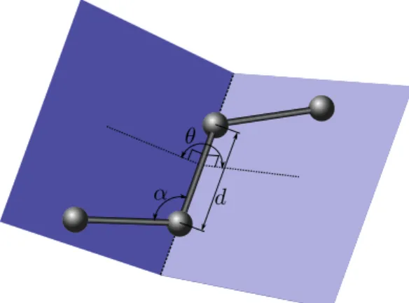
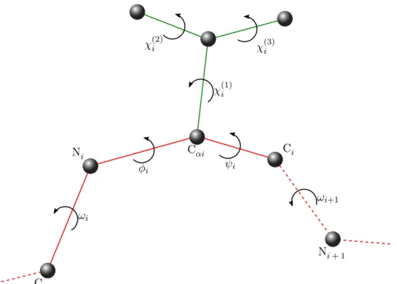
The internal coordinates representation addresses the redundancy existing in the cartesian coordinates model. Knowing the atomic bonds of the protein, the confor-mation of the protein can be fully described using only bond lengths, bond angles, dihedral angles, and the position and orientation of a single frame attached to an atom (See Figure 1.5 for illustration):

• a bond length is the distance between two bonded atoms; • a bond angle is the angle between two consecutive bonds;

(21)

θ

α _d

Figure 1.5: Illustration of the internal coordinate representation parameters. d is a bond length. α is a bond angle. θ is a dihedral angle.

• dihedral angle, also called bond torsion angle, is the angle formed by a group of four consecutively bonded atoms around the central bond.

Using forward kinematics, those parameters allow to recover the cartesian coordi-nates model when needed [Spong 2005].

This representation allows to reduce the number of DOFs by doing quite rea-sonable assumptions. A statistical analysis of protein structures reveals that bond lengths and bond angles are constrained to characteristic values at equilibrium. As a consequence, those parameters can be removed from the list of DOFs and considered constant [Scott 1966, Engh 1991]. This is called the rigid geometry as-sumption. Thus, the protein conformation is fully described by the vector of its dihedral angles. This representation is widely used by algorithms to sample the conformational space. It is worth noticing that the internal coordinates are not dependant on a particular reference frame, so the conformations of a protein can easily be compared using this model.

1.2.3 Dimensionality reduction

Internal coordinates together with the rigid geometry assumption drastically reduce the number of degrees of freedom required to model proteins. Yet, for typical problems involving proteins, it is common to reach more than 1000 dihedral angles. Exploring such a high-dimensional conformational space is challenging. Different strategies have been used to further reduce the dimensionality of the search space. One possible approach is to use stronger assumptions and consider some subset of DOFs as constant. For example, in molecular docking problems, it was very common to consider that the protein is rigid and that only the ligand is flexible [Leach 2001] even though it has been shown that this assumption leads to unre-alistic solutions [Cavasotto 2005]. Some more reunre-alistic assumptions based on prior knowledge of the protein [Jones 1997, Apostolakis 1998, Pak 2000] target the dihe-dral angles that contribute the most to the motions of the molecule and consider

(22)

1.2. Protein modeling 11

the rest of the protein as rigid. Some studies have tried to automatically identify which parts of the protein can be considered rigid using methods based on rigidity theory [Thomas 2013].

A second approach to reduce the dimensionality of the search space is to map its DOFs into a lower-dimension space using statistical knowledge of the studied system [Fodor 2002, Van Der Maaten 2009]. Principal component analysis (PCA), for instance, can be used to analyze molecular dynamics simulations data (see para-graph 1.4.1) to capture important collective motion features [Mu 2005, Altis 2007]. Another method allowing to capture collective motion features is the isometric fea-ture mapping (IsoMap) method [Tenenbaum 2000, Das 2006]. More recently, the locally scaled diffusion map method (LSDMap) was created to take into account local variation of molecular configuration space [Rohrdanz 2011]. Those methods require obtaining prior data on the system which can be a difficult process in itself. A third approach to reduce dimensionality is to use normal mode analysis [Cui 2005]. It has been shown that large-amplitude motions in proteins are re-lated to low-frequency normal modes [Hinsen 1998, Tama 2001]. This method does not require prior knowledge or data about the studied protein as the NMA can be performed from a single conformation. It has been applied to find transition pathways between conformations [Kirillova 2007].

1.2.4 Coarse grained models

A more radical approach to reduce the number of dimensions is to consider a coarse grained representation of the molecular system. All-atom representations of the protein allow for accurate energy calculation but at a high computational cost. Coarse grained representations sacrifice structural details in order to reduce the dimensionality of the search space and improve the speed of energy calculations. Such representations change both the coordinates of the conformational space and the corresponding potential energy model. Coarse graining may for example take into account only a few representative atoms of each residue. It allows to drastically reduce the number of DOFs in the problem without reducing the flexibility of the system. Of course, this comes at a cost. The loss of the full atom representation introduces inaccuracies that can yield unrealistic results.

Early coarse grained representations were lattice-based. C_α were the only rep-resented atoms and were only allowed to lie on a lattice [Taketomi 1975, Yue 1995, Hinds 1994, Kolinski 1994, Unger 1993]. By making the conformational space dis-crete, those models pushed the limits of computational capabilities of protein mod-eling. They are still used to deal with very large protein systems out of reach of current computational capabilities of more accurate models [Dotu 2011].

Off-lattice coarse grained models are also very commonly used [Tozzini 2005]. They differ in how many atoms are represented in the backbone and in the side-chains. One-bead models use a single coarse grained atom to represent an entire amino acid residue. For instance, The G¯o model is a very simple representation where one bead represents each amino acid at the position of its C_α[Taketomi 1975].

(23)

In this model, the interactions between beads are the attractive and repulsive forces based on the protein native structure. This native centric view of the protein makes this kind of model only useful in specific contexts. The G¯o representation has been widely used in the protein folding community and many variations of this representation are still used [Clementi 2008]. Another example of one bead model is the BLN model. Each residue is modeled by one bead that can have one of three labels depending on its chemical properties (B for hydrophobic, L for hydrophilic, N for neutral). These labels mainly determine the interactions between beads [Oakley 2011]. The BLN model is described more in depth in Sec-tion 4.4.2. Two-bead models allow to roughly represent the side-chains and their interactions. A second bead is placed at the β-carbon or at the centroïd of the side-chain [Bahar 1997, Mukherjee 2004, Khalili 2004, Zacharias 2003]. Models with more beads also exist, each bead increasing the accuracy of the model while adding DOFs. For instance, the OPEP coarse grained model uses up to 6 beads to repre-sent amino acids [Sterpone 2014]. The MARTINI coarse grained model also uses a variable number of bead for each type of amino acid [Monticelli 2008].

1.3 Energy landscape

1.3.1 Physical theory

Explicitly modeling protein dynamics is a complex process considering the size of those systems. In the classical approximation, Newton’s laws theoretically allow to predict protein dynamics making it possible to fully understand their folding process or their interactions with other molecules. Given the position of every atoms in the system and their initial velocity, the energy of the system can be computed as the sum of the kinetic energy and potential energy. Newton’s equations then give the dynamics of the system. The kinetic energy is only dependent on the momenta of the atoms in the system: it is a quadratic function of the atoms’ velocities and masses. The potential energy, on the other end, is much more complex. It depends on the positions of the atoms, ie. on the configuration of the system, which in the absence of explicit solvent molecules is just the conformation of the protein. If we look at the potential energy as an altitude, the potential energy function can be seen as an hypersurface drawn over the conformational space. This hypersurface is called the potential energy landscape [Wales 2004, Schön 2009].

The potential energy term is so complex that obtaining a good approximation is a whole field of research, as will be explained in paragraph 1.3.2. Furthermore, analytically solving the Newton’s equations of motion is not feasible for systems as complex as proteins. It is possible to numerically solve these equation with a very small time step (see paragraph 1.4.1). Yet, the study of the energy landscape of a protein gives important information about the states of that protein. Minima of the energy landscape correspond to locally stable, or metastable conformations of the system. Of course, it should be mentioned that atomic fluctuations actually forbid the system to stop in a single stable conformation. Instead, the system wiggles

(24)

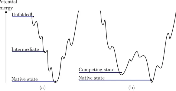
1.3. Energy landscape 13 Potential energy Native state Competing state Unfolded Intermediate Native state (a) (b)

Figure 1.6: (a) Simplified view of a funnel-like energy landscape. High energy values correspond to unstructured state of the system while the lowest energy region corresponds to the native state energy basin. (b) Simplified view of a landscape with two competing low energy basins joined by a low energy saddle.

around an energy minimum and eventually jumps to another basin, slowly reaching a lower energy region in which the system will be trapped for a longer time. Low energy basins surrounded by high energy regions corresponds to the stable states of the system. Many proteins have a unique stable state corresponding to their biologically active state, ie. their native state. In this case, the underlying energy landscape is funnel-like with one deep energy basin corresponding to that native state. An example of a funnel-like landscape is shown in Figure 1.6 (a). Because of structural frustrations, the landscape is typically rugged with a high number of local minima [Onuchic 1997, Onuchic 2004]. Even though most proteins have a funnel-like energy landscape, some protein can have multiple competing low energy basins with eventually low energy transition paths between them [Okazaki 2006]. An example of a landscape with multiple accessible basins is shown in Figure 1.6 (b). Some other proteins even have very flat energy landscape with a lot of competing states. These proteins are called intrinsically disordered proteins.

1.3.2 Energy functions

Obtaining a good approximation of the potential energy surface is not trivial. Great effort are made to produce more and more accurate energy functions.

Energy functions are usually built as the sum of several terms:

E = Ebond+ Eangle+ Etorsion+ Eelectro+ EvdW

where E_bond, E_angle, and E_torsion are terms concerning the local interactions of atoms constrained by atomic bonds. They respectively enforce the constraints on

(25)

the bond lengths, the bond angles, and the dihedral angles. E_electro and E_vdW are terms concerning the long range interactions of atoms which are not neighbor in the molecular topology (not connected by one or two consecutive atomic bonds). Eelectro corresponds to the electrostatic interactions between atoms, and E_vdW corresponds to their van der Waals interactions [Bondi 1964]. Examples of well known physical force fields include the AMBER [Kollman 1997] and CHARMM [Brooks 2009] force-fields.

Protein systems are not lying in vacuum. They are surrounded by a solvent (usu-ally water). Even though the contribution of the solvent to the potential energy can be taken into account using similar energy terms as those mentioned before, it highly increases the complexity of the system as every molecule of water must be modeled at the cost of additional DOFs and high computational time. A sim-pler way to deal with the solvent is to use an implicit model [Roux 1999]. The solvent molecules are omitted in the system representation and a specific energy term Esolvent is added to the potential energy. Esolvent may thus be a complicated function of the conformation of the protein. The most used implicit solvent models are the Coulomb/Accessible Surface Area (CASA), the Poisson-Boltzmann equation (PB), and the Generalized Born model (GB).

In addition to the physics-based energy functions, explained above, knowledge-based functions have been proposed as an alternative approach to evaluate molec-ular conformations. Knowledge-based energy functions, also called statistical en-ergy functions, rely on the growing data that is available nowadays in the PDB to parametrize each term. The Rosetta energy function [Simons 1999, Das 2007] is an example of force field that mixes both physical terms and knowledge-based terms.

Even with relatively simple energy terms, the evaluation of the energy potential for a protein system is quite computationally expansive. This high cost is detrimen-tal to protein sampling methods that extensively rely on energy evaluation. Many strategies can be adopted to improve the speed of energy calculations. An example of such a strategy is to perform a pairwise decomposition of the energy function [Dahiyat 1997, Gaillard 2014] for which internal energies of residues and interaction energies between pairs of residues are precomputed. The energy function is con-structed in such a way that it is a sum of those internal energies and residue-residue interaction energy.

Coarse grained energy function were created together with the coarse grained models mentioned in paragraph 1.2.4 with the aim to reduce computational cost with respect to all-atom representations. They have the advantage to be much faster to compute and to yield much smoother energy landscape. Many coarse grained energy functions incorporate some knowledge about the native states of the protein, rewarding native contacts while penalizing non-native ones [Clementi 2008]. This kind of native structure bias is very commonly used in the field of proteins folding. On the other hand, some coarse grained energy functions do not incorporate prior knowledge of the protein structure to compute energy. This kind of function is especially used in de-novo structure prediction where they yielded several successes [Mukherjee 2004, Colubri 2004]. Nevertheless, although they are good alternatives

(26)

1.4. Computational methods for the exploration of protein

conformations 15

to all-atom energy functions computationally speaking, they introduce inaccuracies and often fail to discriminate good structures from bad ones (e.g. [Bowman 2009]).

1.4 Computational methods for the exploration of

pro-tein conformations

Different algorithms exist to explore the conformational space and the associated energy landscape of a protein systems. This section gives an overview of the most used ones, and also presents some more recent algorithms originating from the field of robotics.

1.4.1 Molecular dynamics

Molecular Dynamics (MD) methods simulate the classical dynamics of a molecular system in order to approximate in silico what could be the temporal evolution of the configuration of the system. They rely on a model, usually an all-atom one in cartesian coordinates, associated with a potential energy function. Starting from an initial configuration C₀ with randomly assigned initial velocities, it builds a trajectory of configurations [Frenkel 2001]. This trajectory can then be analyzed, for instance to observe a folding process or to understand what are the characteristic states of the system. The initial configuration of the system is built depending on the goal of the simulation. For example, if the goal of the simulation is to understand protein folding, an extended configuration of the protein will be built and used as the initial state. If the goal of the simulation is to observe the transition of the protein from one state to another, a configuration of the protein in one of those states (coming from X-ray diffraction, or from NMR for instance) will be chosen to start the simulation. The initial velocities are randomly chosen depending on the simulated temperature. At each step of the simulation, the configuration Ct+δt of the system at time t + δt is computed from the configuration Ct at time t by numerically solving Newton’s equations of motion: accelerations of every atom can be computed from the gradient of the potential energy allowing to compute the new configuration and velocities of the system after a time δt.

MD simulations can be used in many different cases. An observable can be defined and measured during the simulation giving an estimate of its real value, or the sequence of configurations can be stored to be analyzed. A big advantage of MD simulation over other types of algorithms applied to sample a protein confor-mational space is that MD gives access to an actual trajectory of the system with configurations and energy values, but also with the underlying velocities. These data allow to compute many different properties such as the free energies which offer a statistical view of the energy landscape.

Although MD is very often used to study protein systems, it is computationally very demanding. The choice of the time step δt is crucial for the accuracy of the simulation and a typical choice for protein systems is a value around 1-2

(27)

femtosec-16 Chapter 1. Scientific Context

onds. This very small time step is a big limitation. In practice, only simulations covering nanoseconds or a few microseconds can be performed in feasible time (typ-ically several days/weeks). This duration has to be compared with the time scale of protein’s reactions. For example, protein folding can last from a few milliseconds for the fastest proteins to several seconds for slower and larger ones. For other pro-cesses, like the transition of a protein from one state to another competing state, it can even be harder: the transition process might be quite fast, but the simulation may spend a substantial amount of time trapped in the energy basin of the initial state before the transition can be observed.

For proteins with complex energy landscapes, basic MD has very limited sampling capabilities compared to other algorithms. It spends most of its sim-ulation time in low energy regions of the conformational space while interest-ing regions denotinterest-ing state transitions have higher energies. Different meth-ods have been developed to overcome this problem. The replica exchange MD (REMD) [Sugita 1999] reproduces the ideas of the parallel tempering method [Geyer 1991] (See 1.4.2) to apply them to MD: several isothermal MD simu-lations are run with different temperatures and the simusimu-lations are regularly swapped between temperatures with some acceptance probability. REMD allows crossing high energy barriers and has been widely used for protein simulations [Periole 2007, Zhang 2005, Nguyen 2005, Beck 2007]. Another approach that allows MD to cross high energy barriers is steered MD (SMD) [Suan Li 2012, Park 2004]. This methods simulates a pulling force that will hopefully cause the conformational changes necessary to cross the energy barrier and observe the desired trajectory. Metadynamics is another powerful method that improves MD sampling capabilities [Laio 2002]. It is based on two ideas: a dimensionality reduction is performed by the use of carefully chosen collective coordinates, and the energy force field is biased by the addition of a Gaussian term that progressively fills already explored regions of the landscape.

1.4.2 Monte Carlo methods

The Monte Carlo (MC) method [Metropolis 1953] is a stochastic algorithm. It explores the conformational space with a random walk favoring low energy regions. Starting from an initial configuration, a sequence C₁, . . . , Cn of configurations is built. At each step, or move, the last configuration Ct is randomly perturbed. The obtained configuration C_candidate is accepted or rejected with a probability P such as P =    e −∆E kbT _{if ∆E > 0} 1 otherwise (1.1) where ∆E is the potential energy variation from Ctto Ccandidate, kbis the Boltzmann constant, and T is a temperature parameter. This test is called the Metropolis Criterion. The temperature parameter T allows to control the greediness of the exploration. At low temperature, the simulation will quickly converge to a nearby

(28)

energy minimum but won’t be able to cross high energy barriers, while at high temperature, the simulation will be able to occasionally cross high energy barriers, exploring a larger region of the energy landscape at the cost of a longer convergence time.

Unlike MD where the changes between two consecutive conformations are com-puted from Newton’s laws of motion, the perturbations performed at each MC step are random. They do not even have to be realistic moves as long as they are coupled with the Metropolis Criterion mentioned earlier. Nevertheless, the choice of a move scheme strongly affects the efficiency and the quality of the sampling. The moves should provide a good coverage of the conformational space while being computa-tionally efficient and with a good acceptance rate. This subject will be discussed more in depth in chapter 2. For chain molecules such as proteins, a few standard move classes can be mentioned. The pivot move perturbs a single dihedral angle randomly chosen in the polypeptide chain. This move is the most popular and sim-ple one. The concerted rotation is another type of move which has the particularity to be local and only affect a small number of atoms in the system: a dihedral angle from the main-chain of the polypeptide is randomly perturbed and the six following dihedral angles are computed in order to ensure that the succeeding atoms of the chain do not move (this is in general possible and will be explained more in detail in chapter 2).

Although MC has higher sampling capabilities than MD, it nevertheless loses kinetic information. The resulting trajectory cannot be considered as an actual trajectory but only as a sampling of the conformational space and only statistical analysis of the results can be performed. However, when performed carefully, ie. when MC moves satisfy detailed balance1, the distribution of the conformations is guaranteed to follow the Boltzmann distribution and statistical properties of the system, like free energies, can still be computed accurately.

Even though MC simulation is generally faster than MD to explore the con-formational space, processes like protein folding or like transitions between states are still very hard to observe using this method. Similarly to what is done in MD, the replica exchange MC (or parallel tempering) method simultaneously runs multi-ple MC simulations with different temperatures [Swendsen 1986, Earl 2005]. In this context, each simulation is called a walker. Regularly, a swap of temperature is tried between the walkers. Other variants can be cited: umbrella sampling [Torrie 1977] and energy landscape flattening [Zhang 2002] try to bias the transition test to favor transitions between energy basins while basin hopping [Wales 1997] and simulated annealing [Kirkpatrick 1983] aim at finding the global minimum of the energy land-scape.

1

Detailed balance requires that each transition x → y is reversible, i.e. for every pair of states

x, y, the probability of being in state x and transitioning to state y must be equal to the probability

(29)

1.4.3 Robotics-inspired algorithms for the exploration of the con-formational space

The exploration of the conformational space of a protein has similarities with an-other widely studied problem from the robotics community: the motion planning problem. This problem, whose goal is to compute the motion to take a robot from one configuration to another, has been the subject of active research for more than forty years [Latombe 1991, Choset 2005] and has yield significant advances in do-mains such as industrial manufacturing and computer animation. The algorithms solving motion planning problems are called planners.

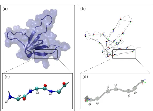
A parallel can be drawn between the notions of configuration space in robotics and conformational space in structural biology. The configuration space [Lozano-Perez 1983] is the space of all the possible configurations that a robot can take. Its dimension depends on the chosen representation for the robot and it is usually constrained by obstacles. A protein can be considered as a robot with multiple articulated bodies. Therefore, the configuration space of that robot corre-sponds to the conformational space of the protein system and the obstacles are the regions of the conformational space where the protein is in collision with itself or with other molecules. The similarities can even go further when we notice that the internal coordinates representation is actually very similar to the representation of an articulated kinematic chain in robotics.

Those similarities have been used to apply robotics-inspired algorithms to solve computational structural biology problems since the 1990s [Parsons 1994] and many adaptations of motion planning algorithms have been created in recent years [Moll 2008, Al-Bluwi 2012]. These algorithms are mainly variants of the Prob-abilistic Roadmap (PRM), the Rapidly-exploring Random Tree (RRT), and the Expansive-Spaces Trees (EST). The basic principles of these three algorithms are presented below. As the goal of the motion planning problem is to find the trajectory between two configurations, the main way they are applied in structural bioinfor-matics is to find transition trajectory between different conformations of proteins. Though, as will be explained in Chapter 3, these algorithms can be adapted to explore the energy landscape.

1.4.3.1 PRM

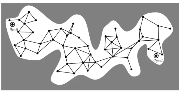
The Probabilistic Roadmap algorithm [Kavraki 1996] is a stochastic algorithm in-troduced in the 1990’s. If many variations of the PRM algorithm have been created over the years to improve its efficiency ([Amato 1998, Wilmarth 1999, Siméon 2000, Sánchez 2003, Geraerts 2004]), the basic principle remains the same. Adaptations of the PRM to work on molecular systems were developed very early [Singh 1999, Amato 2003] and the framework has been improved to work with large proteins [Thomas 2005, Thomas 2007, Molloy 2014]. The algorithm works in two separate phases: the roadmap construction, and the query phase.

(30)

Roadmap construction phase First, a roadmap is built by performing random samples from the configuration space. Sampled configurations are checked for col-lisions and collision-free configurations are added to the roadmap as nodes. This process is repeated until n nodes have been created. Then, for each node, the k closest neighbors are identified and a local planner is called to try to connect each neighbor to the node. When the connection is successful, an edge is added to the roadmap.

This process builds a graph, called the roadmap (see Figure 1.7), which tends to cover the whole configuration space and gives connectivity information between configurations. If the construction principle of the roadmap is very simple, it is nevertheless the most important step of the PRM algorithm and every operation must be performed carefully:

1. Collision checking is quite straightforward for a robot system, but when work-ing with a molecular system, a simple collision test is not sufficient to ensure a realistic conformation. The potential energy needs to be taken into account to ensure more realistic conformations, for example, by choosing a rejection threshold.

2. A uniform sampling of the configuration space is a good approach for low di-mensional problems, but in many cases, and especially in the case of protein systems where the conformational space is very high-dimensional, a biased sampling is required. For instance, in [Molloy 2014], samples are built using a database of backbone fragments from native protein structures to increase the chances of sampling low energy conformations. Furthermore, the fragments are chosen using a heuristic that aims to maximize conformational space cov-erage.

3. The local planner that determines if two nodes can be connected is also critical. A simple strategy could be to do a linear interpolation on each DOF between the two nodes and to check for collisions/energy with a regular check step. More sophisticated approaches can be adopted involving local sampling and probabilistic transition test like the Metropolis Criterion (1.1).

Query phase The goal of the query phase is to use the roadmap built in the first stage of the algorithm to solve the motion planning problem. The initial and the goal configurations are connected to their nearest neighbors in the roadmap and a graph search algorithm such as Dijkstra’s shortest path [Dijkstra 1959] or A* [Hart 1968] is used to find the shortest path connecting the two configurations. The particularity of the PRM algorithm is that the same roadmap can be used for multiple queries potentially saving a lot of computing time.

However having a good configuration space coverage can be a difficult task. If the initial or the goal configuration cannot be connected to the roadmap, or if they fall in disconnected components of the roadmap, the query fails. Though,

(31)

qinit

qgoal

Figure 1.7: Illustration of a PRM roadmap. The white areas represent collision-free regions of the configuration space.

it does not mean that there is no realistic path between the two configurations. For that reason, the PRM algorithm is not a complete algorithm. PRM is said to be probabilistically complete, ie. when the number of sampled nodes approaches infinity, the probability that PRM finds a solution if one exists approaches 1.

1.4.3.2 RRT

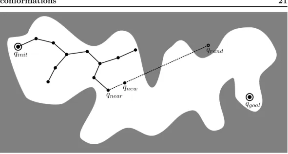
The RRT algorithm is a tree-based motion planner [Lavalle 1998, LaValle 2001]. Starting from an initial configuration, it iteratively grows a tree of configurations until the goal configuration can be connected to the tree. Once this condition is met, a simple tree search gives the solution path. The exploration strategy of RRT uses an implicit Voronoï bias to quickly expand toward unexplored re-gions of the space [Lindemann 2004]: a random configuration q_randis sampled from the configuration space and the next candidate node qnew is created by moving an incremental distance δ from the node qnear in the direction of qrand (see Fig-ure 1.8), e.g. using a linear interpolation. This new configuration is accepted if it is collision free and if it can be connected to qnear using the local planner. The details of the algorithm and the adaptations for molecular simulations are ex-plained in Chapter 3. The RRT algorithm has been shown to be probabilistically complete [LaValle 2001]. Many variants of this algorithm have been developed to improve its efficiency and/or to treat specific problems. We will only mention RRT-connect [Kuffner Jr 2000], real-time RRT [Bruce 2002], resolution complete RRT [Cheng 2002], obstacle based RRT [Rodriguez 2006], or RRT* [Karaman 2010]. Two variants of the RRT algorithm have been developed with a particular focus on problems coming from structural biology: ML-RRT [Cortés 2008, Cortés 2010b], and T-RRT [Jaillet 2008, Devaurs 2013b].

(32)

1.4. Computational methods for the exploration of protein conformations 21 qinit qgoal qnear qnew qrand

Figure 1.8: Illustration of an iteration of the RRT algorithm. A node q_rand is sampled and the closest node in the tree qnear is pulled toward qrand to create qnew. If qnew is collision free, it is added to the tree. This process is repeated until qgoal can be connected to the tree.

1.4.3.3 EST

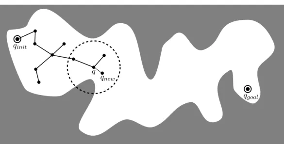
Similarly to the RRT algorithm, the EST approach grows a tree of configurations in the search space [Hsu 1997, Hsu 2000, Hsu 2002]. At each iteration, a configuration

q is chosen in the tree with some probability P (q). Then, a random configuration qnew is sampled from a uniform distribution in the neighborhood of q (see Fig-ure 1.9). If this configuration is collision-free and can be connected to q using the local planner, it is added into the tree. The EST algorithm has also been shown to be probabilistically complete [Hsu 2000]. EST is a very general algorithm as the choice of the probability function P that will determine which node will be ex-tended can be adapted depending on the goal. Furthermore, if the basic version of EST samples q_rand from a uniform distribution in the neighborhood of q, this step can easily be biased to yield a more efficient sampling of the search space. This is particularly interesting to explore the high-dimensional conformation space of protein systems where the sampling can be restricted to realistic moves. Chapter 2 gives some examples of such kind of moves and an example of implementation of EST will be developed in Chapter 3. A successful variant of the EST algorithm is KPIECE [Sucan 2012]. In this version of the algorithm, the probability function

P is built in such a way that nodes that are the most likely to improve the space

(33)

qinit

qgoal

qnew

q

Figure 1.9: Illustration of an iteration of the EST algorithm. A node q_newis sampled in the neighborhood of a chosen node q. This process is repeated until qgoal can be connected to the tree.

1.5 Computational Protein Design

Protein design is the process of finding the amino acid sequence to build a protein with the desired function. Considering the huge number of possible designs (there are 20N possible sequences to try for a N amino acid long protein), it is not possible in practice to synthesize and test all of them. Computational protein design (CPD) has been developed as a tool to identify the most promising candidates and is prob-ably the most practical option to speed up that process. Over the last decades, sig-nificant progress has been made, from early redesign of protein cores [Hurley 1992, Harbury 1995, Desjarlais 1995, Betz 1996, Dahiyat 1996] to complete de novo pro-tein design [Dahiyat 1997, Kuhlman 2003]. A good review of the progress made up to a decade ago is presented in [Lippow 2007]. The range of problems addressed by CPD has been extended to the improvement of protein drug properties [Luo 2002], the redesign of protein-protein interfaces [Clark 2006, Fleishman 2011] and the cre-ation of a metal-protein interface [Yosef 2009, Der 2012]. Other important results are presented in [Röthlisberger 2008, Jiang 2008, Siegel 2010].

1.5.1 The CPD problem

As we explained in section 1.1.2, the interaction of a protein with its environment is mainly determined by the spatial arrangement of its composite atoms. For this reason, the CPD problem is usually expressed as follows: find sequences of amino acids that will fold into the desired spatial arrangement. Solving this problem is very complex and is usually decomposed in four different stages:

(34)

1.5. Computational Protein Design 23

the goal arrangement of the protein. This stage requires expert knowledges of proteins and of the desired interactions. Therefore, it is hard to fully automate this stage. It is usual to rely on known protein scaffolds and only concentrate on designing the geometry of the active site. This phase also defines the constraints on the protein, like required amino acids near the active site, or a set of mutable amino acid positions.

2. The second stage is the search for the sequence that will fold into the de-fined scaffold. Since solving the folding problem while exploring the sequence space is extremely complex, CPD solves a simplified instance The addressed problem consists in searching for the sequence that will best stabilize the goal structure. This search is expressed as an optimization problem. An objec-tive function encoding the stability of the goal structure is defined, and the solution sequence is the one that minimizes this function. Of course, it does not guarantee that the protein will actually fold into the desired structure. Therefore, in general, the search usually looks for multiple probable solutions with values close to the global minimum.

3. The third stage is the analysis of the results. It consists in performing molec-ular simulations (such as MD, MC, etc.) in order to check how the candidate sequences perform in more realistic conditions. Depending on the result of this stage, the initial problem might need to be reworked and another iteration of stages one and two might be needed.

4. Finally, the most promising candidate sequences can be synthesized for ex-perimental validation. The feedback from this stage can be used to refine the solution sequence, or to step back to previous stages of the process.

In the next sections, the focus will be on the second stage of the CPD process, which is the most related one with this thesis.

1.5.2 The search space

The space explored during the second phase of the CPD process is the product of two heterogeneous components:

• A discrete component corresponding to all the possible amino acid sequences. For instance, if the CPD problems has to find the amino acid for every position in the sequence in a 100-amino-acid-long protein, it results in 20100 possible sequences. The reader should notice that exploring such a space entirely is out of reach of current computational capabilities.

• A continuous component corresponding to the conformational space for each of the possible sequences. The dimension of this component corresponds to the number of DOFs in the chosen representation of the protein.

(35)

An important part of the work in the definition of a CPD problem is to reduce the search space in order to make the problem tractable. This work includes the selection of mutable residues, the constraints on the amino acid types depending on the position, and the conformational variability of the side-chains: which side-chain are actually allowed to move. Other approximations are usually applied to further reduce the complexity of the problem.

First, a statistical analysis of the amino acid side-chain conformations in pro-tein databases reveals that side-chains only populate a reduced number of clusters around low-energy conformations. This result was exploited to build databases of side-chain conformations called rotamers. The use of these rotamer libraries transforms a part of the continuous component of the search space into a discrete component where each amino acid has a limited number of possible conformations. It should be mentioned that several works relax this approximation by considering continuous rotamer libraries where fluctuations of side-chains around their equilib-rium positions are taken into account [Gainza 2012].

A second common simplification is the fixed backbone approximation [Ponder 1987]. As the CPD problem aims at optimizing the sequence for a particu-lar backbone conformation, it makes sense to only consider the side-chain variability and to try to fit the amino acids on the backbone conformation corresponding to the designed scaffold. Combined with the previous approximation, the CPD problem is reduced to a search for the optimal rotamers to fit a given backbone. Although these simplifications have enabled significant advances in the CPD community, the treated problem is nevertheless unrealistic. Backbone fluctuations generally have stronger effects on energy than side-chains have. Furthermore, the fact that a sequence minimizes the objective function does not guarantee that the backbone conformation is actually stable for that sequence. It might just lie on the slope of a basin corresponding to a different stable state in the energy landscape.

Several methods have been developed to take the flexibility of the back-bone into account during the CPD process [Georgiev 2007, Fung 2007, Hu 2007, Murphy 2009]. For example, the multi-copy backbone approach simulates the flex-ibility of the backbone by incorporating into the objective function the stability of an ensemble of backbone conformations which are considered to be representative of the designed state [Fung 2008]. Efficient sampling techniques, like the ones men-tioned in paragraph 1.4.3, can also be used to explore the conformational space. For instance in the approach presented in [Kuhlman 2003], sequence optimization phases are alternated with backbone optimization phases.

1.5.3 Current methods for CPD

Even with the approximations mentioned previously (discrete rotamer library and fixed backbone approximation) and using a pairwise decomposable energy function, finding the set of rotamers that minimizes the objective function has been shown to be a NP-hard problem [Pierce 2002]. Both deterministic and stochastic algorithms exist to solve this problem [Wernisch 2000].

(36)

1.5. Computational Protein Design 25

1.5.3.1 Deterministic algorithms

The Dead-End Elimination algorithm (DEE) prunes the search space by iteratively removing rotamers that can be proven not to be part of the optimal solution [Desmet 1992]. The algorithm iterates until no more dead-end rotamer can be found. Although the DEE algorithm does not always reduce the space to one single rotamer sequence, it nevertheless highly reduces the search space allowing a com-plete algorithm like A* [Hart 1968] to be used to find the lowest energy sequence [Leach 1998]. The DEE algorithm has been extended to improve its efficiency and the range of problem it can tackle. More advanced criteria have been added to the original pruning criterion, and variants of the algorithm allow to include some con-formational variability [Goldstein 1994, Pierce 2000, Georgiev 2006, Georgiev 2007, Georgiev 2008].

The Cost Function Network (CFN) is an extension of a mathematical model called Constraint Network where constraints are replaced by cost functions. The CPD problem can also be modeled in a CFN and formulated as a weighted con-straint satisfaction problem (WCSP) where the goal is to find the set of variables (the rotamers) that minimizes the sum of all cost functions (representing the ob-jective function). The algorithm implemented in toulbar2 demonstrated an impor-tant speed-up compared the the DEE/A* algorithms [Allouche 2012, Traoré 2013, Allouche 2014].

1.5.3.2 Stochastic algorithms

If deterministic algorithms have the advantage to guarantee that the best sequence will be found, the complexity of CPD problems make them unusable to design big protein systems. Stochastic CPD algorithms usually cannot guarantee that the best solution will be found, but they are able to find some candidate solutions in a relatively short time [Voigt 2000]. Considering that, with all the approximations made to solve a CPD problem, finding the sequence that minimizes the objective function does not guarantee that this sequence will actually fold into the goal struc-ture, it makes sense to consider other sequences with a good score as equally valid candidate for the design.

The most common stochastic algorithms in CPD use the MC method with its numerous variants. They are similar to the MC method explained in Section 1.4.2 except that they work at two different levels. One level corresponds to the sequence space, where each MC step is performed by changing the sequence and where the Metropolis Criterion (1.1) is applied with the objective function instead of the potential energy function. The other level corresponds to the conformational space, aiming to converge to a minimum energy conformation for the current sequence [Polydorides 2011].

Another type of algorithm used in CPD is based on Genetic Algorithm (GA). GA works by maintaining a population of candidate solutions that will be slowly improved at each iteration by performing operations derived from the biological process of natural selection, including mutations, selections, and crossovers. A