HAL Id: hal-00681688
https://hal.archives-ouvertes.fr/hal-00681688
Submitted on 22 Mar 2012
HAL is a multi-disciplinary open access
archive for the deposit and dissemination of
sci-entific research documents, whether they are
pub-lished or not. The documents may come from
teaching and research institutions in France or
abroad, or from public or private research centers.
L’archive ouverte pluridisciplinaire HAL, est
destinée au dépôt et à la diffusion de documents
scientifiques de niveau recherche, publiés ou non,
émanant des établissements d’enseignement et de
recherche français ou étrangers, des laboratoires
publics ou privés.
M. Materassi, G. Consolini, Emanuele Tassi
To cite this version:
M. Materassi, G. Consolini, Emanuele Tassi. Sub-fluid models in dissipative magneto-hydrodynamics.
Topics in Magnetohydrodynamics, InTech, pp.35, 2012. �hal-00681688�
Sub-Fluid Models in Dissipative
Magneto-Hydrodynamics
Massimo Materassi
1, Giuseppe Consolini
2and Emanuele Tassi
3 1Istituto dei Sistemi Complessi ISC-CNR, Sesto Fiorentino,
2INAF-Istituto di Fisica dello Spazio Interplanetario, Roma,
3Centre de Physique Théorique, CPT-CNRS, Marseille,
1,2
Italy
3France
1. Introduction
Magneto-Hydrodynamics (MHD) describes the plasma as a fluid coupled with the self-consistent magnetic field. The regime of validity of the MHD description of a plasma system is generally restricted to the temporal and spatial scales much larger than the characteristic plasma temporal scales (such as those associated with the plasma frequency, the ion and electrons cyclotron frequencies and the collision frequency), or the typical spatial scales (as the ion and electron inertial scale, the ion and electron Larmor radii and the Debye length). On the large scale, the plasma can be successfully described in terms of a single magnetized fluid by means of generally differentiable and smooth functions: this description of plasma media has met a wide success. However, the last decade of the 20th Century has brought to
scientists’ attention a wide amount of experimental and theoretical results suggesting substantial changes in classical magnetized plasma dynamics with respect to the MHD picture. In particular, two fundamental characteristics of the MHD as a dynamical theory have started to appear questionable: regularity and determinism. The MHD variables are, indeed, analytically smooth functions of space and time coordinates. Physicists refer to this as regularity. Moreover, once the initial conditions are assigned (together with some border conditions), the evolution of the MHD variables is unique: hence MHD is strictly
deterministic. Instead, in in-field and laboratory studies, more and more examples have been
brought to evidence, where irregularity and stochastic processes appear to play a role in magnetized plasma dynamics. This is particularly true when one approaches intermediate and small scales where the validity conditions for the MHD description, although still valid, are no longer valid in a strict sense, or when we are in the presence of topologically relevant structures, whose evolution cannot be described in terms of smooth functions. From now on, the conditions of the MHD variables apparently violating smoothness and/or determinism will be referred to as irregular stochastic configurations (ISC). In the following we remind, in some detail, these experimental and theoretical results pointing towards the existence of ISCs, in the context of space plasmas and fusion plasmas.
In the framework of space physics, it has been pointed out that both the global, large scale dynamics and some local processes related to plasma transport could be better explained in
terms of stochastic processes, low-dimensional chaos, fractal features, intermittent turbulence, complexity and criticality (see e.g. Chang, 1992; Klimas et al., 1996; Chang, 1999; Consolini, 2002; Uritsky et al., 2002; Zelenyi & Milovanov, 2004 and references therein). A certain confidence exists in stating that the rate of conversion of the magnetic energy into plasma kinetic one observed in events of magnetic reconnection is significantly underestimated by the traditional, smooth and deterministic, MHD (see for example Priest & Forbes, 2000 and also Biskamp, 2000). Lazarian et al. (2004) have found an improvement in the calculation of the magnetic reconnection rate by considering stochastic reconnection in a magnetized, partially ionized medium. This process is stochastic due to the field line probabilistic wandering through the turbulent fluid. In a different context, Consolini et al. (2005) showed that stochastic fluctuations play a crucial role in the current disruption of the geomagnetic tail, a magnetospheric process occurring at the onset of magnetic substorm in the Earth’s magnetotail (see, e.g., Kelley, 1989; Lui, 1996). Consistently with the relevance of stochastic processes in space plasmas, tools derived from information theory have been recently applied to describe the near-Earth plasma phenomenology (Materassi et al., 2011; De Michelis et al., 2011). On the other hand, turbulence has been shown to play a relevant role in several different space plasma media as the solar wind (Bruno & Carbone, 2005) or the Earth’s magnetotail regions (see, e.g., Borovsky & Funsten, 2003), etc.
In fusion plasmas, phenomena important as anomalous diffusion induced by stochastic magnetic fields (Rechester & Rosenbluth, 1978) have been suggested to be caused by the appearance of irregular modes similar to ISCs: those modes have been documented since a rather long time (Goodall, 1982). In tokamak machines ISCs observed are mesoscopic intermittent and filamentary structures: recently, studies have shown how such structures might be generated by reconnecting tearing modes triggered by a primary interchange instability (Zheng & Furukawa 2010).
The appearance of ISCs should not be expected as an exceptional condition: indeed, time- and space-regular MHD relies on very precise hypotheses, not necessarily holding in real plasmas. As underlined before, it should be considered that MHD is a long time description with respect to the interaction times of particles. In order to expect a smooth deterministic evolution in time, “fast phenomena” should be ignored, and clearly this cannot be done when “fast phenomena” lead to big changes in the MHD variables themselves, on macroscopic scales, as it happens in the fast magnetic reconnection.
Space regularity requires the scale at which matter appears as granular to shrink to zero, and this is possible under the hypothesis that such scale is much smaller than the typical scale where the MHD variables do vary. However, in turbulent regimes the scale at which the MHD fields vary are so small, that they compare with those scales at which plasma appears as granular.
The phenomenology of plasma ISCs appears to indicate that the role of “fundamental entities” should be played by mesoscopic coherent structures, interacting and stochastically evolving. These stochastic coherent structures (SCS) have been observed in several space plasma regions: in solar wind (Bruno et al., 2001) as field-aligned flux tubes, in the Earth's cusp regions (Yordanova et al., 2005), in the geotail plasma sheet as current structures, 2D eddies and so on (see, for instance, Milovanov et al., 2001; Borovsky & Funsten, 2003; Vörös et al., 2004; Kretzschmar & Consolini, 2006). Recent observations of small-scale magnetic
field features in the magnetosheath transition region (as described in Retinò et al., 2007; Sundkvist et al., 2007) seem to suggest that the dynamics of such coherent structures can be the origin of a coherent dissipation mechanism, a sort of coarse-grained dissipation (Tetrault, 1992a, b; Chang et al., 2003) due to interactions that result non-local in the k-space.
A consistent theory of plasmas in ISC should be a consistent theory of SCSs, valid in a suitable “midland” of the “coupling constant space” (Chang et al., 1978). This “midland of SCSs” should be far from the particle scale (because each SCS involves a large amount of correlated particles), but also some steps under the fluid level (because matter should appear granular and fields irregular).
Furthermore, this “midland” is not the usual kinetic-fluid transition as described e.g. in Bălescu (1997). In fact, the kinetic description is sensible under some weak coupling approximation allowing for a self-consistent Markovian single particle theory to exist, while if mesoscopic coherent structures appear, the correlation length and inter-particle interaction scale are so big that the single particle evolves only together with a large number of its fellows, excluding such weak coupling. Then, if SCSs exist, the kinetic level of the theory does not.
Well far from trying to give a self-consistent theory of the SCS, here we just discuss some models and scenarios retaining some properties that such a theory should have. The approaches discussed here are exactly the application of the philosophy well described by Bălescu (1997) to dissipative processes in the MHD. Probably, a first principle analytical theory of turbulence is going to be out of reach for decades. However, something useful for applications can be developed in a more advanced framework than “traditional” statistical mechanics by introducing elements of chaos or stochasticity, Gaussian or non-Markovian properties, in some “effective” and “sound” models. In this way, one admits a certain “degree of randomness” in the equations, so that the non-Gaussianity of the basic stochastic processes, the role of the non-Markovian equations of evolution, the role of fractal structures and the emergence of “strange transport” are all SCS theoretical features of which one tries to take into account.
The schemes presented here are models with these properties, trying to interpolate between the macroscopic, smooth, deterministic physics of traditional MHD and the mesoscopic, irregular, stochastic physics of “that something else” which has not been formulated yet. Such phenomenological approach is indicated as sub-fluid.
In this chapter three sub-fluid models are described, the metriplectic dissipative MHD, the stochastic field theory of resistive MHD and the fractal magnetic reconnection.
In the first model, the metriplectic dissipative MHD (§ 2), we focus on the relationship between the fluid dynamical variables and the microscopic degrees of freedom of the plasma. The thermodynamic entropy of the plasma microscopic degrees of freedom turns out to play an essential role in the metriplectic formalism, a tool developed in the 1980s encompassing dissipation within an algebra of observables, and here adapted to MHD. It is considered that thermodynamics, i.e. statistics, naturally arises for the description of the microscopic degrees of freedom. Fluid degrees of freedom are endowed with energy, linear and angular momenta, while an entropy function, measuring how undetermined their “mechanical” microscopic configuration is, can be attributed to the microscopic degrees of freedom.
In the second model treated, the stochastic field theory (SFT) (§ 3), the dissipation coefficients appearing in the MHD equations of motion are considered as noise, consistently with the fact that, out of its equilibrium, a medium may be treated statistically. In this way, MHD turns into a set of Langevin field equations. These may be treated through the path integral formalism introduced by Phythian (1977), appearing particularly suitable for non equilibrium statistics. Once the resistive MHD theory is turned into a SFT, transition probabilities between arbitrary field configurations may be calculated via a stochastic action formalism, closely resembling what is usually done for quantum fields. This mimics very precisely the idea of an ISC.
A sub-fluid model of fast magnetic reconnection (FMR) is dealt with in § 4. FMR clearly belongs to the class of phenomena in which classical fields apparently undergo quantum-like transitions in considerably short times: when magnetic field lines reconnect, the field topology is changed and a big quantity of magnetic energy, associated to the original configuration, is turned into the kinetic energy of fast jets of particles. In order to mimic a reconnection rate high enough, a successful attempt may be done relaxing the assumption that all the local variables of the plasma and the magnetic field are smooth functions. In particular, in a standard 2-dimensional Sweet-Parker scenario (Parker, 1957, 1963; Sweet, 1958), one assumes that the reconnection region, where finite resistivity exists, is a fractal domain of box-counting dimension smaller than 2. This allows for a reconnection rate that varies with the magnetic Reynolds number faster than the traditional one.
2. The dissipation algebrized
Dissipation is a crucial element of the physical mechanism leading to ISCs in plasmas, and dissipative terms already appear in the smooth deterministic MHD. Moreover, the presence of dissipation, together with non-linearity, is a fundamental mechanism in order for coherent structures to form (Courbage & Prigogine, 1983).
Many fundamental phenomena giving rise to plasma ISCs in nature, such as turbulence, magnetic reconnection or dynamo (Biskamp, 1993), are often described by MHD models containing dissipative terms. For instance, this can account for the finite resistivity of the plasma and/or the action of viscous forces.
Where does dissipation come from? Ultimately, MHD is derived from the Klimontovich equations, describing the dynamics of charged particles interacting with electromagnetic fields (Klimontovich, 1967). This is a Hamiltonian, consequently non-dissipative, system. Nevertheless, dissipative terms appear in some versions of MHD equations as a heritage of averaging and approximations carried out along the derivation procedure and which have spoilt the original Hamiltonian structure of the Klimontovich system. The presence of dissipative terms reflects a transfer of energy from the deterministic macroscopic fluid quantities into the microscopic degrees of freedom of the system, to be treated statistically, which lie outside a macroscopic fluid description. Such transfer of energy, in turn, implies an increase of the entropy of the system.
If dissipative terms are omitted, on the other hand, one expects the resulting MHD system to be Hamiltonian, with a conserved energy (the constant value of the Hamiltonian of the system) and a conserved entropy. Indeed, the non-dissipative version of MHD, usually
referred to as ideal MHD, has been shown, long ago, to be a Hamiltonian system (Morrison & Greene, 1980). The elements constituting a Hamiltonian structure are the Poisson bracket, a bilinear operator with algebraic properties, and the Hamiltonian of the system, depending on the dynamical variables: in the case of the MHD, these will be defined in the following (see (7) and (9)). The Hamiltonian formulation of the ideal MHD, apart from facilitating the identification of conserved quantitites, or the stability analysis of the equilibria, renders it evident that the dynamics of the system takes place on symplectic leaves that foliate the phase space (Morrison, 1998).
The inclusion of dissipative terms invalidates the Hamiltonian representation: this dissipative breakdown matches the fact that, once dissipation is included, the system becomes “less deterministic” in a certain sense, because there is an interaction with microscopic degrees of freedom that are described in a statistical manner (friction forces are a statistically effective treatment of microscopic stochastic collisions).
Some dissipative systems possess however an algebraic structure called metriplectic, which still permits to formulate the dynamics in terms of a bracket and of an observable, extending the concept of Hamiltonian. Metriplectic structures in general occur in systems which
conserve the energy and increase the entropy. These are the so called complete systems. They are
obtained adding friction forces to an originally Hamiltonian system, and then including, in the algebra of observables, the energy and entropy of the microscopic degrees of freedom. The metriplectic formulation permits to reformulate the dynamics of dissipative systems in a geometrical framework, in which information, such as the existence of asymptotically stable equilibria, may be easily retrieved without even trying to solve the equations.
In order to define what a metriplectic structure is, and apply this concept to the case of MHD, it is convenient to start recalling that, very frequently, one deals with the analysis of physical models of the form
, 1,..., ,i i i
tz F zH F zD i N
(1)
where z is the set of the N dynamical variables of the system (N can be infinite; it is actually a continuous real index for field theories or the MHD) evolving under the action of a vector field FH(z) + FD(z). Such vector field is the sum of a non-trivial Hamiltonian component FH(z)
and a component FD(z) accounting for the dissipative terms. If FD(z) = 0, the resulting system
is Hamiltonian and consequently can be written as
,
,i i i
tz F zH z H z
(2)
where H(z) is the Hamiltonian of the system, and [*,*] is the Poisson bracket, an antisymmetric bilinear operator, satisfying the Leibniz property and the Jacobi identity (Goldstein, 1980). These properties render the Poisson algebra of group-theoretical nature. An immediate consequence of the antisymmetry of the bracket is that ∂tH = [H,H] = 0, so that H is
necessarily a constant of motion.
It is important to point out that, in many circumstances, the Poisson bracket is not of the canonical type. In particular, for Hamiltonian systems describing the motion of continuous media in terms of Eulerian variables, as in the case of ideal MHD, the Poisson bracket is
noncanonical and no pairs of conjugate variables can be identified. For such brackets,
particular invariants, denoted as Casimir invariants, exist. These are quantities C(z) such that [C,F] = 0 for every F(z). Consequently ∂tC = [C,H] = 0 in particular, which shows that
Casimir functions are indeed conserved quantities.
Energy conservation and entropy increase in metriplectic systems are “algebrized” via a generalized bracket and a generalized energy functional. More precisely, a metriplectic system is a system of the form
,
,
,
,i i i i
tz z F z z F z z F z
(3)
where the metriplectic bracket {*,*} = [*,*] + (*,*) is obtained from a Poisson bracket [*,*] and a metric bracket (*,*). The latter is a bilinear, symmetric and semidefinite (positive or negative) operation, satisfying also the Leibniz property (strictly speaking, a symmetric semi-definite bracket (*,*) should be referred to as semi-metric). The metric bracket is also required to be such that (f,H) = 0, for every function f(z), with H being the Hamiltonian of the system: this means that dissipation does not alter the total energy, since this already includes a part accounting for the energy dissipated.
The function F in (3) is denoted as free energy, and is given by ,
F H C (4)
where C is a Casimir of the Poisson bracket, and λ is a constant.
In the cases of interest here, this C is chosen as the entropy of the microscopic degrees of freedom of the plasma, involved in the dissipation.
Let us assume the metric bracket be semi-definite negative (the case in which it is positive is completely analogous). The resulting metriplectic system possesses the following important properties:
- ∂tH = 0, so that the Hamiltonian of the system is still conserved (possibly other
quantities such as total linear or angular momenta can also be conserved);
- ∂tC = λ(C,C), so that, due to the semi definiteness of the symmetric bracket one has
either ∂tC ≥ 0 or ∂tC ≤ 0 at all times, depending on whether λ is negative or positive.
This candidates C to be an equivalent time coordinate wherever it is strictly monotonic with t (Courbage & Prigogine, 1983);
- isolated minima of F are stable equilibrium points.
Metriplectic structures have been identified for different systems as, for instance, Navier-Stokes (Morrison, 1984), free rigid body, Vlasov-Poisson (Morrison, 1986) and, in a looser sense, for Boussinesq fluids (Bihlo, 2008) and constrained mechanical systems (Nguyen & Turski, 2009). An algebraic structure for dissipative systems based on an extension of the Dirac bracket has been proposed by Nguyen and Turski (2001). They have also been used for identifying asymptotic vortex states (Flierl and Morrison, 2011).
Also the visco-resistive plasma falls into the category of complete systems. Indeed, the following version of the visco-resistive MHD equations
2 2 2 1 , 2 , , i k i ik i k i i k k t k j j j i i i i i t j j j j t j j ik k i h i k m n t j ikh mn p B B V V V B B B V B V V B B V s V s V B B T T T T (5)can be shown to possess a metriplectic formulation. In (5) we adopted a notation with SO(3)-indices, which turns out to be practical in this context. We specify that
2 3 m n ik ni mk nk mi ik mn ik mn V
is the stress tensor, with η and ν indicate the viscosity coefficients, κ is the thermal conductivity, T the plasma temperature and s the entropy density per unit mass. In the limit
κ = ζ = ν = σik = 0, one recovers the ideal MHD system treated by Morrison and Greene
(1980), reading:
2 1 , 2 , , . i k i i k i i k t k j j j i i i i t j j j j t j j t j p B B V V V B B B V B V V B V s V s (6)Morrison and Greene (1980) showed that the system (6) can indeed be cast in the form (2). This is accomplished first, by identifying the dynamical variables zi with the fields
(B(x,t),V(x,t),ρ(x,t),s(x,t)) (here, the space coordinate x labels the dynamical variables and plays the role of a continuous 3-index). The Hamiltonian for ideal MHD is then
2 2 3 , , , , . 2 2 V B H s d x U s
B V (7)The three addenda in the integrand correspond to the kinetic, magnetic and internal energy of the system, respectively. U(ρ,s) is related to the plasma pressure and the temperature as: 2 U, U. p T s (8)
The Poisson bracket giving rise to the frictionless (6) through the Hamiltonian (7) is given by:
3 1 , 1 1 1 . i i i j j kmn kmn ijk m n ijk m n i i jmn i i ikj m n i i i k f g g f f g d x s s V s V f g f g B B V B B V f g g f f g V V V V V
(9)This bracket possesses Casimir invariants (e.g. Morrison, 1982, Holm et al., 1985), such as the magnetic helicity; particularly relevant in our context, the total entropy is defined as:
3 .
S
sd x (10)S is conserved along the motion of the non-dissipative system (6).
Some observation should be made here about the role of the plasma entropy as a Casimir. Casimir are invariants that a theory shows because of the singularity of its Poisson bracket, which is not full-rank. Typically this can happen when a Hamiltonian system is obtained by reducing some larger parent one, which possesses some symmetry (see, e.g., Marsden & Ratiu, 1999, Thiffeault & Morrison, 2000). In the case of ideal MHD, the reduction which leads to the Poisson bracket (9), is the map leading from the Lagrangian to the Eulerian representation of the fluid (Morrison, 2009a). When the system of microscopic parcels is approximated as a continuum, its (Lagrangian or Eulerian) fluid variables (as the velocity
V(x,t)) pertain to the centre-of-mass of the fluid parcels of size d3x within which they may be
approximated as constants. However, fluids are equipped with some thermodynamic variable, as the entropy s per unit mass here, which represent statistically the degrees of freedom relative-to-the-centre-of-mass of the parcels in d3x. In the Lagrangian description,
the value of the entropy per unit mass is attributed to each parcel at the initial time, and remains constant, for each parcel, during the motion. In the Eulerian description, the total entropy appears as a Casimir, after the reduction, and the symmetry involved in this case is the relabelling symmetry, which is related to the freedom in choosing the label of each parcel at the initial time. In this respect, it is worth recalling that this reduction process implies a loss of information (e.g. Morrison, 1986) in the sense that, through the Eulerian description, one can observe properties of the fluid at a given point in space, but cannot identify which parcel is passing at a given point at a given time.
In a sense, this observation renders the metriplectic a sub-fluid description, because those microscopic degrees of freedom interact with the continuum variables through the role of S in (10) in the metric part of the evolution.
If the dissipative terms are re-introduced into Eq. (6) and one goes back to Eq. (5), a complete system is obtained, in the sense that H in (7) doesn’t change along the motion (5), while entropy S in (10) is increased (Morrison, 2009b).
Let us illustrate the metriplectic formulation for the system (5). The non-dissipative part of the dynamics is algebrized through the Hamiltonian (7) and the Poisson bracket (9). As far as the construction of the free energy F in (4) is concerned, the entropy S is taken as the Casimir C, whereas the metric bracket reads:
, 1 3 2 1 1 1 1 1 1 1 1 k k i i k m m n ikmn k n i i k m m n ikmn k n f g f g d x T T s T s f f g f T V V V T s V T s f f g f T B B B T s B T s
. (11)This metric bracket can be decomposed into two parts. A “fluid” part, corresponding to its first two terms, which was shown to produce the viscous terms of the Navier-Stokes equations (Morrison, 1984), and a “magnetic” part, which accounts for the resistive terms. The proof that the above metric bracket satisfies the properties required by the metriplectic formulation has been given in Materassi & Tassi (2011). The SO(3)-tensors needed are defined as: 2 , 3 . ikmn ni mk nk mi ik mn ik mn h ikmn ikh mn
The bracket (11) together with the free energy functional
2 2 3 , , , , 2 2 V B F s d x U s s
B V (12)produces the dissipative terms of the system (5).
Thanks to the metriplectic formulation, it appears evident that the dynamics of the complete visco-resistive MHD takes place on surfaces of constant energy but, unlike Hamiltonian systems, it crosses different surfaces of constant Casimirs. Choosing C = S, it becomes evident that the fact that the dynamics does not take place at a surface of constant Casimir reflects of course the presence of dissipation in the system, and in particular the increase in entropy.
Free extremal points of F in (12) (i.e., configurations at which one has F = 0 regardless other
conditions) correspond to equilibria of the system (5) (even if other equilibria are possible). These can be found by setting to zero the first variation of F and solving the resulting equation in terms of the field variables. These equilibrium solutions are given by
0, 0, , constant eq eq eq eq eq eq T p Ts U V B (13)(since it has been obtained as extremal of the free energy functional, this solution is also an equilibrium for ideal MHD). The equilibrium (13) is rather peculiar because it corresponds to a situation in which all the kinetic and magnetic energy have been dissipated and converted into heat. It ascribes a physical meaning to the constant λ, that corresponds to the
opposite of the homogeneous temperature the plasma reaches at the equilibrium. Other equilibria with non trivial magnetic or velocity fields can in principle be obtained by considering Casimir constants other than the entropy, and a different metric bracket, or simply by constraining the condition F = 0 onto some manifold of constant value for
suitable physical quantities. Moreover, the boundary conditions for the system to work in this way must be such that all the fields behave “suitably” at the space infinity. All the results are obtained for a visco-resistive isolated plasma: indeed, all the algebraic relationships invoked hold if V, B, ρ and s show suitable boundary conditions, rendering visco-resistive MHD a “complete system”.
Such metriplectic formulation conserves, in addition to the energy H, also the total linear momentum P, the total angular momentum L and the generator of Galileo’s boosts G, which are defined by:
3 , 3 , 3 . d x d x t d x
P V L x V G x VAbout these quantities P, L and G, it should be stressed that, besides modifying the scheme with other quantities conserved in the ideal limit, more interesting equilibria than (13) may be identified by conditioning the extremization of F to the initial finite values of the Galilean transformation generators.
3. Sub-fluid physics as noise: A stochastic field theory for the MHD
The metriplectic theory of the MHD discussed in § 2 clarifies how the dissipative part of the dynamics must be attributed to the presence of statistically treated degrees of freedom, through their entropy. On the one hand, the metriplectic MHD gives a role to the statistics of the medium properties; on the other hand, local equilibrium and space-time-smoothness of field variables are still assumed. In the sub-fluid model presented in this paragraph, the statistical nature of the microscopic degrees of freedom is cast into a form going beyond the local equilibrium condition. In particular, strong reference to plasma ISCs is made.
Plasma ISC dynamics resembles more closely a quantum transition than a classical evolution: the idea presented here is that localized occurrence of big fluctuations in the medium probably initiate and determine those quantum-like transitions of the variables B and V. If the fluctuations of the medium are treated as probabilistic stirring forces, or noises, a totally new scenario appears.
The formalism turning those considerations into a mathematical theory was introduced in Materassi & Consolini (2008); then, an application of it to the visco-resistive reduced MHD in 2 dimensions was obtained in Materassi (2009).
Let’s consider the resistive incompressible MHD equations:
, j j ijk i i i h t j j j kh i j j jki i i t j k B B V V B J J p V V V B (14)(the choice of incompressible plasma is done for reasons to be clarified later). ζ is the resistivity tensor and p is the plasma pressure. The dynamical variables are the fields V and
B. The viscosity ν is assumed to be zero. The form of ζ and p, and of the mathematical
relationships among them (necessary to close the system (14)), depend on the micro-dynamics of the medium. Usually, constitutive hypotheses provide the information on the microscopic nature of the medium (Kelley, 1989). When the (at least local) thermodynamic equilibrium is assumed, the constitutive hypotheses read something like:
T,... ,
p T, 0, (15)
being T the local temperature field. Then, some heat equation is invoked for T, requiring other constitutive hypotheses about the specific heat of the plasma.
The aforementioned procedure will only give ζ and p regular quasi-everywhere. Instead, in the sub-fluid approach presented here, irregularities of ζ and p are explicitly considered by stating that these local quantities are stochastic fields, and by assigning their probability density functions (PDF). The probabilistic nature of the terms ζ and p will be naturally transferred to B and V through a suitable SFT. The following vector quantities are defined
, i, i : ijk i h i i j khJ J p (16)these Ξ, Δ, and Θ are considered as stochastic stirring forces, and their probability density
functional is assigned as some Q[Ξ,Δ,Θ]. The resistive MHD equations are then re-written as
the following Langevin field equations:
iid , , , , , , . j j i i i i t j j j jki i i i t j j k B B V V B V V V B Q Ξ Δ Θ Ξ Δ Θ (17)This scheme, clearly, is not self-consistent because the PDF of the noise terms must be assigned a priori, as the outcome of a microscopic dynamics not included in this treatment and not predictable by it. Plasma microscopic physics will enter through some PDF Pdyn[ζ,p]:
as far as Pdyn[ζ,p] keeps trace of the plasma complex dynamics, this represents a (rather
general) way to provide constitutive hypotheses. Then, the positions (16) are used to construct mathematically the passage:
,p iidPdyn,p
Ξ Δ Θ, ,
iidQΞ Δ Θ, , .A closed form for Q[Ξ,Δ,Θ] should be obtained consistently with any microscopic
dynamical theory of the ISC plasma, from the very traditional equilibrium statistical mechanics to the fractional kinetics reviewed in Zaslavsky (2002).
Due to the presence of the stochastic terms Ξ, Δ, and Θ two important things happen: first of
(17), each corresponding to a particular realization of Ξ, Δ, and Θ (Haken, 1983); then B and V
can be arbitrarily irregular, because they inherit stochasticity from noises; they will possibly show sudden changes in time or non-differentiable behaviours in space, as it happens in ISCs. The description of such a system may be given in terms of path integrals (Feynman & Hibbs, 1965). The positions (16) and their consequence (17) are chosen because they reproduce exactly the Langevin equations treated in Phythian (1977), on which this model is based.
The construction introduced in the just mentioned work is the definition of a path integral scheme out of a suitable set of Langevin equations. One starts with a dynamical variable ψ, with any number of components, undergoing a certain equation with noises. Then, another variable χ is defined, referred to as stochastic momentum conjugated to ψ. In this way, it is possible to define a kernel
0 , 0 0 [ , ; , ) , , t t i L d A t t N t t e (18)so that any statistical outcome of the history of the system between t0 and t is calculated as:
0
[ , ; , ) .
F
d
d A t t FIn the kernel in (18) the quantity L(ψ,χ) is referred to as stochastic Lagrangian of the system. In Phythian (1977) the key result is a closed “recipe” to build up L(ψ,χ) out of the Langevin equation of motion.
The same procedure may be applied to the system governed by the Langevin equations (17); these may be turned into a SFT by identifying the dynamical variables ψ of the system as B and V, and introducing as many stochastic momenta χ as the components of ψ (Materassi &
Consolini, 2008):
, .
B V Ω Π
The variables Ω and Π are two vector quantities representing the stochastic momenta of B and V respectively. A stochastic kernel A[Ω,Π,B,V;t0,t) is constructed by involving a noise factor
3 0 0 [ , , , ; , ) , , : t t i d d x C t t d d d Q e
Ξ Ω Θ Π Δ Π B Ω Π B V Ξ Δ Θ Ξ Δ Θ (19)all the statistical dynamics of the resistive MHD interpreted as a SFT is then encoded in the kernel
3 0 0 , , , 0 0 0 0 [ , , , ; , ) , [ , , , ; , ) , , , , . t t i d L d x A t t N t t C t t e L Ω Π B V Ω Π B V Ω Π B V Ω Π B V Ω B Π V Ω V B B V Π V V (20)The quantity L0(Ω,Π,B,V) is interpreted as the part of the Lagrangian of the SFT not
containing noise terms. L0 shows only space- and time-local terms, always: as it is stressed in
Chang (1999), the integration of the noise term C[Ω,Π,B,V;t0,t) brings terms in L that are
non-local in space and in time, due to the self- and mutual correlations of noises. Those terms will be collected in a noise-Lagrangian LC, so that all in all one has:
3 0 3 0 , , , 0 , , , 0 0 0 [ , , , ; , ) , , [ , , , ; , ) , . t C t t t i d L d x i d L d x C C t t e L L L A t t N t t e Ω Π B V Ω Π B V Ω Π B V Ω Π B VThe form of Q[Ξ,Δ,Θ], hence of C[Ω,Π,B,V;t0,t), may render the SFT long-range correlated
and with a finite memory: these conditions of the ISC plasmas described by such a SFT is what encourages people to work through the techniques of dynamical renormalization group (Chang et al., 1978). Possibly, the stochastic momenta may be eliminated, so that one obtains a kernel W involving only physical fields
0 0
[ , ; , ) [ , , , ; , ) .
WB Vt t
dΩ
dΠAΩ Π B Vt t (21)Once W[B,V;t0,t) has been obtained, the calculation of processes in which the magnetized
plasma changes arbitrarily, from an initial configuration (B(t0),V(t0)) = (Bi,Vi) to a final one
(B(t),V(t)) = (Bf,Vf), may be done, for any time interval (t0,t): the rate of such transitions
should be calculated as i i f f 0 i 0 i f f , , 0 , , [ , ; , ) t t . t t P d d W t t
B V B V B B V V B B V V B V B V (22)As a further development of Materassi & Consolini (2008), a complete representation à la
Feynman of such processes is to be derived from the SFT, with a suitable perturbative theory
of graphs.
In order to arrive to a closed expression for a stochastic action at least in one example case, hereafter a toy model is reported, in which Ξ, Δ and Θ are assumed to be Gaussian processes
without any memory, and δ-correlated in space. This hypothesis is surely over-simplifying for a
plasma in ISC, since there are experimental results stating the presence of non-Gaussian distributions (Yordanova et al., 2005), and also of memory effects (Consolini et al., 2005). Nevertheless, the Gaussian example is of some use in illustrating the SFT at hand, because a Gaussian shape for Q[Ξ,Δ,Θ] allows for the full integration of C[Ω,Π,B,V;t0,t), and the explicit
calculation of W[B,V;t0,t) from A[Ω,Π,B,V;t0,t) in (21). The probability density functional
Q[Ξ,Δ,Θ] is obtained via a continuous product out of distributions of the local values of the
fields Ξ, Δ and Θ of Gaussian nature; for instance, the PDF of the local variable Ξ(x,t) reads:
2 0 3 , , , 3 , , a t a t t t . q t e x Ξ x Ξ x x Ξ x (23)The quantity aΞ(x,t) indicates how peaked the distribution qΞ(Ξ(x,t)) is, i.e. how deterministic
plasma. Formally equal distributions qΔ(Δ(x,t)) and qΘ(Θ(x,t)) describe the local occurrence
of the values of Δ and Θ. From (23), the expression of the noise kernel C[Ω,Π,B,V;t0,t)
defined in (19) can be calculated explicitly (Materassi & Consolini, 2008), and the noise Lagrangian LC(Ω,Π,B,V) determined in a closed form:
2 0 2 2 2 2 0 , , , 4 4 C i L a i a a Ω Ω Π B V Ω Π B B Π Π Θ Π B Δ Π . (24)This noise Lagrangian is space-local and does not contain any memory term, because the PDF Q[Ξ,Δ,Θ] was constructed as the continuous products of infinite terms, each of which representing the independent probability qΞ(Ξ(x,t))qΔ(Δ(x,t))qΘ(Θ(x,t)). The total Lagrangian
is the sum of the noise term LC(Ω,Π,B,V) and of the “deterministic” addendum L0(Ω,Π,B,V)
presented in (20). The sum L0 + LC gives rise to a perfectly local theory. The total Lagrangian
L0 + LC gives a kernel A[Ω,Π,B,V;t0,t) that is the continuous product of the exponentiation of
quadratic terms in Ω and Π, so that the calculation (21) is an infinite-dimensional Gaussian path integral, which is again feasible. This means that, under the hypothesis (23) on Ξ, and similar assumptions on the two other noises Δ and Θ, the calculation of the stochastic evolution kernel can be done in terms of pure “physical fields” B and V, obtaining
W[B,V;t0,t). If the calculation is performed to the end, the expression of W[B,V;t0,t) reads:
3 0 0 0 2 0 0 2 0 0 ' , 0 0 0 0 2 2 2 1 0 2 2 2 1 0 2 [ , ; , ) ' , , , , ; , , ' , ln 1 1 . t t i d L d x a a a a a a S t t N a a a p t t e L i ia ia p p B V B B B B B B B V B V B B V B B V B V V V B V V V B (25)The functions ζ0 and p0 are defined as the ensemble expectation value of the homonymous
stochastic variables. The expression (25) is ready to be used in (22) to calculate the transition probabilities between arbitrary field configurations. The quantity N’ in (25), whatever it looks like, will not enter the calculations of processes like (22), since it doesn’t depend on V and B, and will be cancelled out. Last but not least, consider that the functions defining noise statistics, i.e. aΞ, aΔ, aΘ, ζ0 and p0, do enter the Lagrangian as “coupling constants”.
Intrinsic limitations of the proposed scheme can be recognized.
First of all, no discussion has been even initiated yet about the convergence of all the quantities defined.
There is an apparent “necessity” of making the choice (16) in order to follow the scheme traced in Phythian (1977). It could be useful to extend the reasoning presented here to other forms of the Langevin equations so to avoid the positions (16) and work directly with ζ and
p as stirring forces in (14).
It is also to mention that the problem of defining a good functional measure is still to be examined, by studying the consistency condition of a Fokker-Planck equation for the SFT, starting for example with the Lagrangian density (25), obtained under drastically simplifying hypotheses.
A comment is deserved by the choice of the incompressible plasma hypothesis. The MHD as a dynamical system is given by (5): in the absence of incompressibility, the mass density ρ is a distinct variable on its own, with a proper independent dynamics. In the stochastic theory à
la Phythian each dynamical variable should satisfy a Langevin equation, in which noise is in
principle involved. Now, altering the equation for ρ with noise could invalidate the mass conservation, which is a big fact one would like to avoid. Hence, the “sacred principle” of non-relativistic mass conservation ∂tρ + ∂·(ρV) = 0 is saved excluding ρ from dynamics,
rendering it a pure parameter of the theory, via incompressibility. The compressible case could be studied considering the local mass conservation a constrain to be imposed to the path integrals as it happens in quantum gauge field theories (Hennaux & Teitelboim, 1992). Last but not least, the fourth equation in (5) has not been considered at all in this scheme: in Phythian’s scheme plasma thermodynamics must be discussed in some deeper way before enlarging the configuration space of stochastic fields to the entropy s.
4. Fractal model of fast reconnection
Among the many interesting fast and irreversible processes occurring in plasmas, magnetic
reconnection is surely one of the most important (see e.g. Biskamp, 2000; Birn and Priest,
2007). The name “magnetic reconnection”, originally introduced by Dungey (1953), refers to a process in which a particle acceleration is observed consequently to a change of the magnetic field line topology (connectivity). Being associated to a change in the magnetic field line topology, the magnetic reconnection process involves the occurrence of magnetic field line diffusion, disconnection and reconnection and it is also accompanied by plasma heating and particle acceleration, sometimes termed as dissipation (actually, in this case dissipation means transfer of energy from the magnetic field to the particle energy, both bulk motion energy, the term ρV2/2 in the integrand in (7), and thermal energy, the term U(ρ,s) in the
same expression of H; in the context of metriplectic dynamics, dissipation is simply the transfer of energy into the addendum U(ρ,s)).
The traditional approach to magnetic reconnection is based on resistive MHD theory. In this framework one of the most famous and first scenarios of magnetic reconnection, able to make some quantitative predictions, was proposed by Parker (1957) and Sweet (1958). The Sweet-Parker model provides a simple 2-dimensional description of steady magnetic reconnection in a non-compressible plasmas (see Figure 1). In this model there are two relevant scales: the global scale L of the magnetic field and the thickness Δ of the current sheet (or of the diffusion region). The main result of such a model may be resumed in the very-well known expression for the Alfvèn Mach number MA,
1/2
0
/ ,
A m m A
M R R LV (26)
where Rm is the Lundquist number (often referred as magnetic Reynolds number), VA is the
Alfvén velocity and is the resistivity.
Fig. 1. A schematic view of 2-dimensional geometry for the Sweet-Parker reconnection scenario
Indeed, being a measure of the electric field normalized by the global electric field, i.e.
/ /
A A A
M V V E V B, (27)
the Alfvén Mach number MA, reported in Eq. (26), provides an estimate of the reconnection
rate, which is generally expressed in terms of the electric field at the reconnection site.
The typical Lundquist number Rm in astrophysical and space plasmas is Rm >> 106, implying
reconnection rates MA << 10-4. These reconnection rates are too slow to explain the explosive
nature of several space processes associated with the occurrence of reconnection, so that the
Sweet-Parker model is considered not suitable to explain reconnection in space plasmas. In the course of the time, to overcome such a limitation of the Sweet-Parker model several other models have been proposed. Among these models one of the most successful is the
Petscheck model (Petscheck, 1964), where the diffusion region (associated with the current
sheet) is greatly reduced in length and the energy conversion is associated with the presence of two pairs of standing slow-modes. As a result, the reconnection rate in terms of Alfvénic Mach number is 8ln A m M R (28)
Although several other models have been proposed (see e.g.: Birn and Priest, 2007), some recent MHD simulation have shown that, when the Hall effect is included, it is possible to obtain fast magnetic reconnection rates, which are independent on the current sheet or reconnection region size. For instance, Huba & Rudakov (2004) obtained a reconnection rate
MA ≤ 0.1 in the case of Hall magnetic reconnection.
All the above approaches to magnetic reconnection move from the assumption that plasma media can be viewed as noncollisional fluid. This assumption is clearly valid when the inherent local fluctuations x of any local field X are negligible with respect to the large scale
means, 1 2 2 1 10 , x X (29)
being x = X – <X>. Conversely, recent observations evidenced that space plasmas are
characterized by an intrinsic stochastic character, and that in many situations turbulence is present. This is for instance the case of interplanetary space plasmas, such as the solar wind, and the Earth’s magnetotail current sheet, characterized by stochastic and turbulent fluctuations of the same order of magnitude of the average fields.
Several attempts have been done to include the stochastic and turbulent nature of the plasma
media and to discuss its effects on the magnetic reconnection process (see e.g. Yankov, 1997;
Lazarian & Vishniac, 1999). The common point of such models is the idea that as a consequence of the inherent stochasticity and/or turbulent nature of plasma media, the current sheet and the diffusion region topology cannot be associated with a simple continuous regular medium. Conversely, the current sheet could be imagined like a filamentary, complex and not space-filling region.
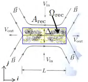
Fig. 2. A schematic view of 2-dimensional geometry for the fractal reconnection model, of size L and Δ, with reconnection area Arec and reconnection active area Ωrec.
In 2007 Materassi & Consolini proposed a revised version of the historical Sweet-Parker model, in which the diffusion/current sheet region, where the magnetic reconnection takes place, is imagined like a fractal object in the plane. The very basic assumption of such a fractal reconnection model is that the reconnection active sites form a not space-filling domain rec contained in the diffusion region of measure Arec, and that such a non-space-filling
domain is characterized by a Hausdorff dimension DH < E, being E the embedding
dimension (here E = 2). Figure 2 shows a schematic view of the 2-dimensional geometry of the diffusion region.
Due to the fractal nature of the diffusion region, the constraint of flux conservation can be written as [ ] [ ], out in eff eff S S V V (30)
where Sin (Sout) is the entrance (exit) surface for the plasma passing through the fractal
domain rec. Here, the flux over the entrance and exit surfaces is given by the following
expression, ˆ [ ] S, S eff S d V
V n (31)where dSis a proper elemental measure for the fractal domain S. Thus, the evaluation of
such fluxes requires an integration over a fractal domain, which can be performed using the definitions by Tarasov (2005, 2006) involving irregular integrals.
According to the results shown in Tarasov (2006), if f is a regular function defined in Rn to be
integrated over a fractal domain characterized by a Harsdorff dimension D < n, then the integration can be performed by introducing a proper weight function D, i.e.
, D A fd f dA
(32)where A is the regular set of dimension n embedding the considered fractal set
When the above integration technique is applied to the condition of flux conservation (30), one gets for the fractal reconnection rate
2 0 2 , in out in out D D FRM in A D D out D M k D L (33)where k is a positive constant such that Vout = kVA, and L are the thickness (typically of the
order of the ion-inertial length) and the length of the diffusion region, respectively, = Dout -
Din is the difference of the Hausdorff dimensions of the projection of the fractal domain in
the direction of the entrance (Din) and exit (Dout) directions, and finally ℓ0 is a reference
microscopic length scale. Such a reference length scale has to be much smaller than the typical
Moving from the above result and assuming k = 1 and Din =Dout = D, Eq. (33) for the fractal
reconnection rate can be reduced to a more simple expression in terms of the Lundquist number Rm:
DD1FRM
A m
M R . (34)
We note that this expression reduces to the standard Sweet-Parker solution of the reconnection rate in the limit D 1 and that the fractal reconnection rate is always higher than the one predicted by the Sweet-Parker model. Furthermore, although in the limit
m
R the reconnection rate predicted by the Petschek-like model results the more efficient, there exists always a certain range of the Lundquist number Rm, depending on the
fractal dimension D, for which the fractal reconnection model is more efficient than the Petschek-like model. The crucial point of a correct estimation and applicability of the above expression stands in the correct evaluation of Din and Dout, which depends on the topology
of the current sheet.
In passing we note that when the above scenario is applied using typical length scales estimated by in-situ observations of magnetic reconnection in space plasmas, one gets the reconnection rates typically observed and in agreement with the estimated Hall reconnection rate MA ≈ 0.09 (Huba & Rudakov, 2004) assuming a diffusion region shaped as
a filamentary structure mainly aligned to the inflow region (direction i in Figure 2).
The fractal reconnection model described here is not based on first principles, because the non-space filling, self-similar nature of the reconnection region is simply assumed.
The important work necessary for further development will be to give a dynamical sense to the quantities Din and Dout, that here might appear just as convenient fitting parameters.
Studies have been made to regard irregular filamentary structures in plasmas as descending from calculable fluid-model processes (Zheng & Furukawa, 2010).
The feeling is however that it would be very interesting to deduce the fractal nature of the reconnection region from kinetic or microscopic-statistical theories, rather than extracting it from extreme behaviours of the plasma as a fluid.
5. Conclusion
Dissipation consists of the irreversible transfer of energy from the proper MHD variables to the particle degrees of freedom of the plasma, considered as “microscopic” (and usually treated via Thermodynamics). Depending on the spatial and temporal scales on which dissipation takes place, it may activate some “sub-fluid level” of the theory, which interpolates between the continuous system, representing the traditional MHD, and the discrete one, describing the plasma through the motion of its particles. This “sub-fluid” level should probably consist of mesoscopic coherent structures existing because of dissipative process, and evolving through a stochastic (strongly noisy) dynamics. Consequently, the self-consistent theory describing this intermediate level of plasma description is expected to be a theory of SCSs.
In this Chapter, three models to approach this “SCS Theory” have been exposed: metriplectic algebrization of MHD, stochastic field theory and fractal magnetic reconnection.
Each of the three models tries to mimic one aspect of the complete theory of SCSs. The metriplectic MHD presents the non-Hamiltonian algebrization; the SFT for the resistive MHD is characterized by the presence of noise yielding a path integral approach; the fractal model of reconnection admits the irregular nature of MHD fields, involving the fractional calculus.
A large amount of work must still be done to imagine how those three approaches could be combined in a unique framework, the invoked “SCS Theory”, reducing to the three models in different limits: this further research is for sure out of the subject of the work here, in which a flavour had to be given about some characteristics that this “SCS Theory” should have.
As a final remark, we underline that the self-consistent “SCS Theory” should present a sort of scale-covariance, because all the phenomena concerning plasma ISCs do involve multi-scale dynamics. The technique of Renormalization Group will then be naturally applied to such a thory (see e.g. Chang et al., 1992 and references therein). A first direct application of such technique, using the exact full dynamic differential renormalization group for critical dynamics can be found in Chang et al. (1978). The use of Renormalization Group techniques to predict physical quantities to be compared with real spacecraft data is already well established (see e.g. Chang, 1999; Chang et al., 2004), and the results are very encouraging, confirming our idea that any “SCS Theory” has to be based on scale-covariance.
6. Acknowledgements
The authors are grateful to Philip J. Morrison of the Institute for Fusion Studies of the University of Texas in Austin, for useful discussions and criticism. The work of Massimo Materassi has been partially supported by EURATOM through the “Contratto di Associazione Euratom-Enea-CNR”. The work of Emanuele Tassi was partially supported by the Agence Nationale de la Recherche (ANR GYPSI n. 2010 BLAN 941 03). This work was also supported by the European Community under the contract of Association between EURATOM, CEA, and the French Research Federation for fusion study. The views and opinions expressed herein do not necessarily reflect those of the European Commission. Emanuele Tassi acknowledges also fruitful discussions with the "Equipe de Dynamique Nonlinéaire" of the Centre de Physique Théorique of Marseille.
Giuseppe Consolini and Massimo Materassi did this work as a part of ISSI Team n. 185 “Dispersive cascade and dissipation in collisionless space plasma turbulence – observations and simulations”, lead by E. Yordanova.
7. References
Bălescu, R.; (1997). Statistical Dynamics: matter out of equilibrium, Imperial College Press, ISBN: 1860940455, London.
Bihlo, A. (2008). Rayleigh-Bénard Convection as a Nambu-metriplectic problem, Journal of
Physics A, 292001, Vol. 41.
Birn, J.; Priest, E.; (2007). Reconnection of magnetic fields. Magnetohydrodynamics and collisionless theory and observations, Cambridge University Press, ISBN-10 0-521-85420-2, Cambridge, United Kingdom
Biskamp, D.; (1993). Nonlinear Magnetohydrodynamics, Cambridge University Press, ISBN-10 0-521-59918-0, Cambridge, United Kingdom.
Biskamp, D.; (2000). Magnetic reconnection in plasmas - Cambridge Monographs in Plasma Physics, Cambridge University Press, ISBN-13 978-0-521-02036-7.
Borovsky, J.E., and Funsten, H.O.; (2003). MHD turbulence in the Earth's plasma sheet: Dynamics, dissipation and driving, Journal of Geophysical Research, 108, 1284, doi: 1.1029/2002JA009625.
Bruno, R., Carbone, V., Veltri, P., et al.; (2001). Identifying intermittency events in the solar wind, Planetary and Space Science, 49, 1201-1210.
Bruno, R., Carbone, V.; (2005). The solar wind as a turbulence laboratory, Living Reviews in
Solar Physics, 2, 4.
Chang, T.S.; Nicoll, J.F.; Young J.E.; (1978). A closed-form differential renormalization-group generator for critical dynamics, Physics Letters, 67A, 287-290.
Chang, T.; (1992). Low-dimensional behavior and symmetry breaking of stochastic systems near criticality -- Can these effects be observed in space and in the laboratory?, IEEE
Transactions on Plasma Science, 20, 691-694.
Chang, T.; (1999). Self-organized criticality, multi-fractal spectra, sporadic localized reconnections and intermittent turbulence in the magnetotail, Physics of Plasmas, 6, 4137-4145.
Chang, T., Tam, S.W.Y., Wu, C.C. and Consolini, G.; (2003). Complexity forced and/or self-organized criticality, and topological phase transitions in space plasmas, Space
Science Review, 107, 425-444.
Consolini, G.; (2002). Self-organized criticality: a new paradigm for the magnetotail dynamics, Fractals, 10, 275-283.
Consolini, G., Kretschmar, M., Lui, A.T.Y., et al.; (2005). On the magnetic field fluctuations during magnetospheric tail current disruption: a statistical approach, Journal of
Geophysical Research, 110, A07202.
Courbage, M. & Prigogine, I.; (1983). Intrinsic randomness and intrinsic irreversibility in classical
dynamical systems, Proceedings of the National Academy of Science of USA, Vol. 80, pp. 2412-2416, Physics.
De Michelis, P., G. Consolini, M. Materassi, R. Tozzi; (2011). An information theory approach to storm-substorm relationship, Journal of Geophysical Research, vol. 116, A08225, doi:10.1029/2011JA016535.
Dungey, J.W.; (1953). Conditions for the occussrence of electrical discarges in astrophysical plasmas. Philosphical Magazine, 44, 725-728
Feynman, R. P. and Hibbs, A. R.; (1965). Quantum Mechanics and Path Integrals, McGraw-Hill Book Company, ISBN: 0-07-020650-3, New York.
Flierl, G.R. and Morrison, P.J.; (2011). Hamiltonian-Dirac Simulated Annealing: Application to the Calculation of Vortex States, Physica D, pp. 212-232, Vol. 240.
Goodall, D. H. J; (1982). High speed cine film studies of plasma behaviour and plasma surface interactions in tokamaks, Journal of Nuclear Materials, Volumes 1112, 11-22.
Goldstein, H., Poole, C. P. Jr., Safko, J.L.; (1980). Classical Mechanics, Addison-Wesley series in physics, ISBN: 978-0201657029, Newark (CA) USA.
Haken, H.; (1983). Synergetics, an introduction, Springer-Verlag, ISBN: 3-8017-1686-4, Berlin, Heidelberg, New York.