Effort Self-Selection and the Efficiency of Tournaments

HAL Id: halshs-00142876

https://halshs.archives-ouvertes.fr/halshs-00142876

Submitted on 23 Apr 2007

HAL is a multi-disciplinary open access archive for the deposit and dissemination of sci-entific research documents, whether they are pub-lished or not. The documents may come from teaching and research institutions in France or abroad, or from public or private research centers.

L’archive ouverte pluridisciplinaire HAL, est destinée au dépôt et à la diffusion de documents scientifiques de niveau recherche, publiés ou non, émanant des établissements d’enseignement et de recherche français ou étrangers, des laboratoires publics ou privés.

Effort Self-Selection and the Efficiency of Tournaments

Tor Eriksson, Sabrina Teyssier, Marie Claire Villeval

To cite this version:

Tor Eriksson, Sabrina Teyssier, Marie Claire Villeval. Effort Self-Selection and the Efficiency of Tournaments. 2006. �halshs-00142876�

GATE

Groupe d’Analyse et de Théorie

Économique

UMR 5824 du CNRS

DOCUMENTS DE TRAVAIL - WORKING PAPERS

W.P. 06-03

Effort Self-Selection and the Efficiency

of Tournaments

Tor Eriksson, Sabrina Teyssier, Marie-Claire Villeval

Mars 2006

GATE Groupe d’Analyse et de Théorie Économique UMR 5824 du CNRS

93 chemin des Mouilles – 69130 Écully – France B.P. 167 – 69131 Écully Cedex

Tél. +33 (0)4 72 86 60 60 – Fax +33 (0)4 72 86 60 90 Messagerie électronique gate@gate.cnrs.fr

Self-Selection and the Efficiency

of Tournaments

Tor Eriksson

Sabrina Teyssier

Marie-Claire Villeval

JEL-Codes: M52, J33, J31, C81, C91.

Keywords: Tournament, Performance Pay, Incentives, Sorting, Selection, Experiment.

Mots-clés: tournois, rémunération à la performance, incitations, sélection, tri, expérience

We are grateful to E.P. Lazear, A. Ichino, K. Lang, L. Vilhuber, R. Mohr, K P Chen and participants at the NBER Summer Meeting in Boston and a seminar at Academia Sinica (Taipei) for their useful comments and suggestions. Financial support from the Aarhus School of Business and the French Ministry of Research (ACI) is gratefully acknowledged.

a _{Aarhus School of Business, Department of Economics and Center for Corporate Performance,}

Prismet, Silkeborgvej 2, 8000 Aarhus C, Denmark. Email: tor@asb.dk

b _{GATE (CNRS – University Lumière Lyon 2 – Ecole Normale Supérieure LSH), 93, chemin des}

Mouilles 69130 Ecully, France. Email : teyssier@gate.cnrs.fr

c GATE (CNRS – University Lumière Lyon 2 – Ecole Normale Supérieure LSH), 93, chemin des Mouilles 69130 Ecully, France, and Institute for the Study of Labor (IZA), Bonn, Germany. Email :

Abstract

When exogenously imposed, rank-order tournaments have incentive properties but their overall efficiency is reduced by a high variance in performance (Bull, Schotter, and Weigelt 1987). However, since the efficiency of performance-related pay is attributable both to its incentive effect and to its selection effect among employees (Lazear, 2000), it is important to investigate the ex ante sorting effect of tournaments. This paper reports results from an experiment analyzing whether allowing subjects to self-select into different payment schemes helps in reducing the variability of performance in tournaments. We show that when the subjects choose to enter a tournament, the average effort is higher and the between-subject variance is substantially lower than when the same payment scheme is imposed. Mainly based on the degree of risk aversion, sorting is efficiency-enhancing since it increases the homogeneity of the contestants. We suggest that the flexibility of the labor market is an important condition for a higher efficiency of relative performance pay.

Résumé

Lorsqu'ils sont imposés de manière exogène, les tournois possèdent des propriétés incitatives importantes mais leur efficacité globale est réduite par le niveau élevé de la variance de la performance des individus (Bull, Schotter et Weigelt 1987). Toutefois, dans la mesure où l'efficacité de la rémunération à la performance peut être attribuée à la fois à un effet d'incitation et à un effet de sélection parmi les salariés (Lazear 2000), il est important d'analyser l'effet de sélection ex ante des tournois. Cet article relate une expérience destinée à tester si la possibilité donnée aux sujets de choisir entre différents modes de rémunération permet de réduire la variance de la performance en tournois. Nous montrons que lorsque les sujets choisissent d'entrer en compétition, l'effort moyen est plus élevé et la variance inter-individuelle est substantiellement réduite par rapport à un traitement où le même mode de rémunération est imposé. L'auto-sélection, fondée en grande partie sur le degré d'aversion au risque, améliore l'efficience car elle accroît l'homogénéité des compétiteurs. Ceci suggère que la flexibilité du marché du travail est une condition importante pour l'accroissement de l'efficience de la rémunération à la performance.

1. Introduction

The use of promotion tournaments is fairly widespread especially in the higher ranks of firms and organizations. The incentive property of tournaments has been studied extensively in the theoretical literature (Lazear and Rosen 1981; Green and Stokey 1983; Nalebuff and Stiglitz 1983; O'Keeffe, Viscusi, and Zeckhauser 1984; for a survey see McLaughlin 1988). The empirical studies, based on survey or experimental data, are fewer and many survey analyses use sports rather than business data (Prendergast 1999). These studies have confirmed that the tournament efficiency depends on the spread between the winner’s and the loser’s prizes, the number of prizes at stake, the size of the tournament, and the degree of uncertainty faced by the employees.1

However, both theoretical models and empirical studies also point to some factors that limit the incentive effect of tournaments, such as collusion among employees or even sabotage (see Lazear 1989 for a theoretical analysis and Harbring and Irlenbusch 2004 for some experimental evidence). More generally, most laboratory experiments have provided evidence of tournaments being associated with a high variance in effort (see in particular Bull, Schotter, and Weigelt 1987 and Harbring and Irlenbusch 2003; van Dijk, Sonnemans, and van Winden 2001). This variance of effort, which is found to be larger in tournaments than in an equivalent piece-rate scheme, reduces the overall efficiency of tournaments.

The principal aim of this paper is to show that previous experimental evidence regarding the variability of effort in tournaments is misleading because the experiments have not accounted for sorting, that is, that agents typically choose to participate in a tournament. The large

1

Studies based on survey data include Bognanno (2001), Ehrenberg and Bognanno (1990b), Eriksson (1999), Knoeber and Thurman (1994), Main, O'Reilly III, and Wade (1993). Studies based on experimental evidence include Bull, Schotter, and Weigelt (1987), Harbring and Irlenbusch (2003), Nalbantian and Schotter (1997), Orrison, Schotter, and Weigelt (2004), Schotter and Weigelt (1992).

variability observed in earlier studies is usually explained by the game nature of the tournament, which requires the agents to elaborate a strategy that is more cognitively demanding than the maximizing behavior required by a piece-rate system (Bull, Schotter, and Weigelt 1987). Indeed, in addition to the stochastic technology of production, the agents have to cope with strategic uncertainty.2 The use of high-variance strategies may also be related to both the difficulty of the task and the ability of the individuals (Vandegrift and Brown 2003). The hypothesis that we test in this paper is that the variability of effort may be reduced – and thus the efficiency of tournament increased - by allowing people to choose their payment scheme, i.e. allowing them to enter or not the competition. More precisely, we suggest that the observed high variance of effort may be due to the fact that in previous experiments very risk averse or under-confident subjects are imposed such a competitive payment scheme. For example, facing these two sources of uncertainty, some of these subjects “drop-out”, i.e. choose the minimum effort, securing the loser’s prize without bearing any cost of effort, whereas others choose the maximum effort, securing the winner’s prize but with an inefficiently high cost of effort. Had the subjects been given the choice, like in flexible labor markets where people can choose to enter or shy away from competitive occupations, very risk averse subjects would probably not have entered the competition and the overall variance of effort would be lower.

By testing whether the performance variability is reduced by the ex ante sorting effect of tournaments, our paper contributes to a very recent literature about the importance of both incentive and sorting effects in the determination of payment schemes’ efficiency, initiated by

2

The variance of effort is diminished when the subjects play against an automaton choosing the same common knowledge effort level repeatedly, but not when more information is given about the past effort of a human competitor. The observed variance can thus be related to the strategic nature of the game.

Lazear (2000).3 This literature shows that sorting influences economic behavior. Earlier, the sorting function of tournaments has mainly been documented with respect to their ability to select ex post the best performers. However, their ex ante sorting effect is considerably less studied and none of the previous empirical studies have been concerned with the impact of ex ante sorting on the variability of performance.4

To study the ex ante sorting effect of tournaments and its impact on the variability of effort, we have designed a laboratory experiment based on the comparison between a Benchmark Treatment and a Choice Treatment, and involving 120 student-subjects. In the Benchmark Treatment, half of the subjects are paid according to a piece-rate payment scheme and the other half enters pair-wise tournaments. This treatment consists of a one-stage game in which the subjects choose their level of effort knowing their payment scheme and the uncertainty of the environment. We find, in line with earlier experiments, that in this treatment, the variance of effort is substantially higher in the tournament than in the piece-rate payment scheme. In the Choice Treatment, we add a preliminary stage in which the subjects choose between a piece-rate scheme and a tournament. Those who choose the tournament are paired together. In the second stage, each subject decides on his level of effort. In both treatments, the individual outcome depends on both the effort level and an i.i.d. random shock. The difference between

3

In the Safelite study (Lazear, 2000), half of the productivity gain associated with the introduction of variable pay is attributed to its ability to sort the most skilled employees. Experimental tests include Cadsby, Song, and Tapon (2004), and Eriksson and Villeval (2004), on sorting and incentives; Lazear, Malmendier, and Weber (2005) on sorting and social preferences; Bohnet and Kübler (2004) on sorting and cooperation.

4

In the theoretical literature, Fullerton and McAfee (1999) propose an auction design in order to limit the entry into tournaments to selected highly qualified contestants. Hvide and Kristiansen (2003) show, however, that the selection efficiency of tournaments is not necessarily increased by improving the quality of the contestant pool. In the empirical literature, Ehrenberg and Bognanno (1990a) show that higher winners’ prizes attract better players and Knoeber and Thurman (1994) propose setting minimum standards to get rid of the poor performing competitors. Niederle and Vesterlund (2005) and Datta Gupta, Poulsen, and Villeval (2005) identify the importance of gender in the ex ante sorting effect of tournaments. Fershtman and Gneezy (2004) introduce a possibility of quitting in a dynamic tournament with asymmetric players. Bonin, Dohmen, Falk, Huffman, and Sunde (2006) use survey data and show that risk averse individuals are more likely to be sorted into occupations with low earnings risk, and Dohmen and Falk (2005) observe that risk averse subjects prefer fixed payments over piece-rate or tournament schemes.

the two payment schemes emanates from the strategic uncertainty associated with the tournament setting.

By comparing the subjects’ behavior in the two treatments, we can identify the impact of sorting on the average and the variance of effort. We also seek to identify determinants of self-selection. The equilibrium effort level is higher in the tournament than under the piece-rate scheme but the expected utility of both compensation schemes is the same. Hence, risk-neutral subjects should be indifferent between the two schemes. For their part, risk averse subjects can adopt a less risky scheme by choosing the piece-rate scheme. We measure the subjects’ risk aversion by using the lottery procedure proposed by Holt and Laury (2002).

Our experiment delivers three main findings. First, the key novel finding is that the employees’ choice of pay schemes contributes to a considerable reduction in the variance of effort among contestants in the tournament. Second, the average effort is higher when the subjects can select their payment scheme, which suggests that the sorting effect reinforces the incentive effect of both tournaments and variable pay schemes. Third, the subjects self-select mainly according to their degree of risk aversion. A cluster analysis identifies a category of under-confident and hesitant subjects who tend to shy away from competition. The resulting greater homogeneity of contestants improves the overall efficiency of tournaments.

The remainder of the paper is organized as follows. Section 2 presents the theoretical framework and the experimental design. Section 3 gives the experimental procedures. Section 4 describes and analyzes the experimental evidence. Section 5 discusses the results and concludes.

2. Theory and Experimental Design

2.1. The model

Consider an economy with identical, risk-neutral agents. Agent i has the following utility function, separable in payment and in effort:

( ) ( ) ( )

i i i i

U e =u p −c e (1)

with u(pi) concave and c(ei) convex.

The production technology is stochastic and output is increasing in the agent’s effort:

( )

i i

y = f e + ε_i (2)

with f(ei) = ei for the sake of simplicity and εi is an i.i.d. random shock distributed over the interval [-z, +z]. Only individual outcomes are observable; individual effort is not observable, neither by the principal nor the other agents. The cost function is increasing and convex

( )

with s > 0, c(0) = 0, c’(ei) > 0 and c”(ei) > 0.5

In the labor market, some firms pay the agents a piece-rate compensation scheme and other firms use tournaments. If there is a perfect mobility in the labor market at no cost, in the first stage the agents choose their firm (i.e. their payment scheme) and, in the second stage, they decide on their level of effort. Let us first solve the equilibrium effort levels under each mode of payment.

In the piece-rate system, the agent’s payment depends only on his own outcome. The payment consists of a fixed wage, denoted by a, corresponding to an input-based payment and a linear

5

piece-rate, denoted by b, corresponding to an output-based payment. Under this compensation scheme, the agent’s utility function becomes:

2 ( ) . PR i i i i e U e a b y s = + − (4)

The first order condition is:

( )

Thus, the equilibrium effort of each agent under the piece-rate payment scheme depends positively on the incentive, b, as well as the cost scaling factor, s:

* .

2

PR b s

e = (5)

In the firms practicing tournaments, the agents play a non-cooperative game with incomplete information like in Lazear and Rosen (1981). In pair-wise tournaments, two prizes are distributed: W is the winner’s prize allocated to the agent whose outcome is the highest and L is the loser’s prize, allocated to the other agent, with W > L. The magnitude of the difference between the two outcomes does not affect the determination of the winner of the tournament. The agent’s utility is:

( )

_{( )}

( )

( )

The agents being symmetric, the probability to win the tournament, pr(ei,ej), reduces to the

probability that the difference in individual random terms exceeds the difference between individual effort levels: pr e e_i, _j = pr

(

)

( )

( )

(

)

( )

( )

₍

₎

We obtain a pure symmetric Nash equilibrium, where effort increases with the prize spread and decreases with both the cost of effort and the size of the shock distribution:

(

)

Having determined the equilibrium effort level under each payment scheme, we now turn to the first stage problem. The agent chooses his firm by comparing his expected utility under each payment scheme. He is thus indifferent between the two schemes when:

(

)

2.2. The experimental design

The instructions have been kept as close as possible to Bull, Schotter and Weigelt (1987) (see Appendix).

Two treatments. In the Benchmark Treatment, a single decision is made: the choice of the level of effort, knowing the cost function, the distribution of the random term and the compensation rule. An important difference from the set-up in Bull, Schotter and Weigelt (1987) is that in a session, half of the subjects are exogenously and randomly attributed a piece-rate payment scheme and the other half a tournament scheme. The proportion is

unknown to the subjects but they aware of the coexistence of two modes of payment. In contrast, Bull et al. (1987) organized separate sessions in which players were paid either a piece-rate or according to a tournament. We wish to keep the social environment comparable with that of the Choice Treatment in which both schemes coexist in the same session in unknown proportions. The game is repeated 20 times.

The Choice Treatment is similar to the Benchmark except that in the first stage of each period, the subjects choose to be paid according to either a piece-rate scheme or a tournament scheme. Those who have opted for the tournament are pooled together and paired. In case of an uneven number of contestants, one subject is randomly chosen and paid according to a piece-rate scheme; he is informed of this before deciding on his level of effort. There is no mobility cost, i.e. the subjects are free to move to the other payment scheme in each new period at no cost. The design of this game enables between-subject but not within-subject comparisons since each treatment is played by different subjects. The latter would have required submitting all the subjects to the exogenous piece-rate scheme, then to an exogenous tournament, then to the choice treatment. It would then have been necessary to alternate between the various treatments to control for potential order effects within the Benchmark and between the Benchmark and the Choice Treatments. Our design is simpler and allows the subjects to play more repetitions of a same treatment.6

Matching protocol. Unlike most experiments on tournaments, here we adopt a stranger matching protocol. This is motivated by the constraint of the Choice treatment: if we had used a partner matching protocol, a subject who is willing to choose the tournament but who is

6

We took care of using similar pools of subjects in both treatments. The average age of the subjects is 20,9 years and the average safety index is 5.3 in both subgroups; Kolmogorov-Smirnov tests indicate that the distribution of age and safety index are not different between treatments. The proportion of men is 45% in the Benchmark and 47% in the Choice Treatment. A Wilcoxon test accepts the equality between treatments.

paired with a person who always chooses the piece-rate, would be prevented from competing throughout the game. A drawback of our matching protocol is, however, that we reinforce the complexity of the tournament game due to conjectural variations, making it harder to make inferences about the opponent’s behavior. If errors in inferences were the source of the greater variability of effort in tournaments, this should entail a greater variability of effort in our design than in standard games. However, this should not affect the comparison between treatments. 7

Parameters. Effort can take any integer value in the set: e_i∈

{

}

function, s = 150, so that . The random shocks vary in the interval [-40,+40]. In

the tournament, the winner’s prize has been set at W = 96 and the loser’s prize at L = 45. In the piece-rate scheme, the fixed wage, a, amounts to 45 and the piece-rate, b, is equal to .52, meaning that each unit of outcome gives .52 to the agent. These values ensure that the certain payment is the same under both schemes. Without such a fixed wage equal to the loser’s prize, it could be rational for a risk averse agent to choose the tournament and a minimum effort in order not to bear the consequences of a negative random shock on wages under a purely linear piece-rate scheme. Therefore, with our design, only the strategic uncertainty makes a difference between the two schemes.

( )

/150

i i

c e =e

Given these values, and assuming the agents to be risk neutral and rational, those who are paid according to a piece-rate scheme should provide the effort eiPR* = 39, according to equation

(5); those who enter the tournament should provide the effort eiT* = 48, according to the pure

strategy Nash equilibrium in equation (9). The players should be indifferent between the two

7

Bull, Schotter and Weigelt (1987) reject the errors in inference explanation of the variance: in fixed pairs, giving the subjects a feedback on the effort chosen by their opponent does not reduce the variance of effort.

payment schemes since the expected utility of both is the same (EUiPR = EUiT = 55), but if

choosing the tournament they have to work harder.

Elicitation of risk aversion. The above predictions hold for risk-neutral subjects. One would expect that risk averse subjects i) reduce their effort level under each mode of payment and ii) are more likely to stay out of the tournament to avoid the strategic uncertainty linked to the competition (Lazear and Rosen 1981). To elicit the risk aversion of our subjects, we used the lottery procedure proposed by Holt and Laury (2002).

At the end of the sessions (in order not to influence the game), the subjects filled out a questionnaire with 10 decisions (see the instructions in Appendix). Each decision consists of a choice between two paired lotteries, “option A” and “option B”. The payoffs for options A are either €2 or €1.6, whereas the riskier options B pay either €3.85 or €0.1. In the first decision, the probability of the high payoff for both options is 1/10. In the second decision the probability increases to 2/10. Similarly, the chances of receiving the high payoff for each decision increases as the number of the decision increases. When the probability of the high payoff is high enough, subjects should cross over from option A to option B. Risk neutrality corresponds to a shift at the fifth decision, while risk loving subjects are expected to move earlier and risk averse subjects as from the sixth decision. The subjects made 10 decisions but only one was selected at random for payment.

3. Experimental Procedures

The experiments have been conducted at the GATE laboratory, Lyon, France. The experiment was computerized, using the Regate software (Zeiliger 2000). We recruited 120 under-graduate students from three business or engineering schools, trying to guarantee a fair gender distribution in each session (46% of male participants in total). Six sessions with 20 subjects in

each have been organized; 3 for the Benchmark Treatment and 3 for the Choice Treatment. Thanks to the 20 repetitions of the game, we collected a total of 2400 observations.

Upon arrival, each subject was randomly assigned a computer. Instructions were distributed and read aloud. Attached to the instructions was a sheet displaying the decision costs associated with each possible effort from 0 to 100. Questions were answered in private. The participants had had to answer a series of questions about the computation of payoffs under each payment scheme. The experiment started once all the participants answered correctly. No communication was allowed.

In the Benchmark Treatment, at the beginning of the session and for its whole duration 10 subjects were attributed the piece-rate scheme and 10 the tournament scheme. In the Choice Treatment, in each period they had to tick either the “mode X” (piece-rate) box or the “mode

Y” (tournament) box to choose their payment scheme for the current period. In both

treatments, they selected their effort (“decision number”) by means of a scrollbar. This being done, they had to click a button to generate their “personal random number” that was added to their effort choice to constitute their individual outcome (‘result”). Under the tournament scheme, the computer program compared the outcomes of the two contestants in each pair and determined who was to receive the winner’s prize (“the fixed payment M”) and who to get the loser’s prize (“the fixed payment L”). In case of a tie, a fair random draw determined the allocation of prizes among the pair members. At the end of the period, each subject received a feedback on his payoff and in case of a tournament, on the difference between his outcome and his competitor’s outcome. In each new period, the pairs involved in a tournament were randomly reconstituted.

After the completion of the 20 periods, the risk aversion post-experimental questionnaire was distributed and read aloud. Subjects noted on a sheet of paper the option they chose for each of the 10 lottery decisions. After all participants had made their decisions, each subject had to throw a ten-sided die twice: once to select the decision to be considered and a second time to determine her payoff for the option chosen, A or B.

All the transactions, except the lottery, were conducted in points, with conversion into Euros at a rate of 80 points = €1. Payment consisted of the sum of payoffs during each period plus the lottery payment and a €3 show-up fee. On average, the subjects earned €17.4. The sessions lasted approximately one hour, excluding the lottery draw and payment that was made in private in a separate room for confidentiality.

4. Experimental Results

4.1. Mean and Variance of Effort

Table 1 displays summary statistics about the mean and the distribution of effort by payment scheme and by treatment.

First, we check whether we observe in our Benchmark treatment, like in the previous experiments, both a higher mean and a greater variance of effort under the tournament than under the rate pay scheme. In this treatment, the average effort is 46.5 under the piece-rate scheme and 53.3 in the tournaments. Both numbers are significantly above the equilibrium effort levels (39 and 48, respectively; t-test, p=0.000). As predicted, the agents exert more effort in a competitive setting (Mann-Whitney U test, p=0.000). As regards the variance of effort, our results corroborate those of previous experiments. Averaging over all

the periods, the total variance is 369 under the piece-rate scheme and 652 in tournaments. Thus the variability of effort is clearly higher under the competitive scheme.

Table 1. Summary statistics on average level and variance of effort

Average effort Mean variance of effort

Periods All 1 1-10 11-20 All 1 1-10 11-20

Piece-rate Benchmark Tr. Choice Tr. 46.5 50.5 55.7 47.6 48.9 51.3 44.0 49.7 368.9 227.9 388.1 192.4 380.3 221.9 354.8 231.7 Tournament Benchmark Tr. Choice Tr. 53.3 61.6 60.0 65.8 55.6 63.4 50.9 59.8 652.3 258.2 663.8 319.4 674.4 238.4 633.5 259.7 30 35 40 45 50 55 60 65 70 1 2 3 4 5 6 7 8 9 10 11 12 13 14 15 16 17 18 19 20 Periods Piece-Rate - Benchmark Tournament - Benchmark e*PR e*Tour Piece-Rate - Choice T Tournament - ChoiceT

Fig.1. Evolution of the effort decisions by treatment and by mode of payment over time

Next, we turn to consider the influence of the possibility given to the subjects to choose their payment scheme. Table 1 and Figure 1 reveal a substantial increase of the average effort from 53.3 in the Benchmark Treatment to 61.6 in the Choice Treatment. Interestingly, average effort also increases from 46.5 in the Benchmark to 50.4 for the agents who choose to be paid

a piece-rate. As a consequence, the differences relative to the equilibrium effort values are even larger when agents self-select. As for the tournaments, we note that while the subjects on average play the equilibrium effort in the last four periods in the Benchmark Treatment, this behavior cannot be observed in the Choice Treatment although there is a slight decline in effort over time. The choice of the payment scheme is associated with a slower convergence to equilibrium.

Table 1 and Figure 2 also show a dramatic change in the variability of effort when agents self-select. Comparing the Benchmark with the Choice Treatment, we find that the variance under the piece-rate diminishes from 368.9 to 227.9 (-38.2%) and the variance in the tournament decreases from 652.3 to 258.2 (-60.4%). Not only is the variability of effort lower when agents self-select, but now the tournament cannot be considered as more unstable than the piece-rate. Levene’s robust test statistic rejects the hypothesis of equality of variance between the tournament and the piece-rate in the Benchmark Treatment (z=48.93, p<0.000) but accepts it in the Choice Treatment (z=.135).

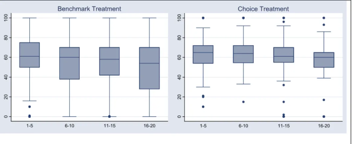
0 2 0 4 0 6 0 8 0 1 0 0 1-5 6-10 11-15 16-20 Benchmark Treatment 0 2 0 4 0 6 0 8 0 1 0 0 1-5 6-10 11-15 16-20 Choice Treatment

Fig.2. Dispersion of effort in the tournaments by treatment and category of periods

Figure 2 displays the dispersion of effort in tournaments in each treatment. The distribution of effort in tournaments in the Choice Treatment is characterized by the following. The median

(indicated by the horizontal line) is slightly higher than in the benchmark. The distribution of effort (given by the quartiles, the grey bars) is more concentrated around the median when agents can self-select, whereas effort is more dispersed below the median when they cannot. The adjacent values (the vertical lines) are closer to the median, meaning in particular that contestants chose a zero effort less often (7 observations out of 564) than in the Benchmark Treatment (45 observations out of 600).

The variability of effort across the game may be explained by both a time-varying behavior (learning dimension) and time-invariant inter-individual characteristics (heterogeneity dimension). To gauge the relative importance of these two dimensions, in Table 2 we decompose the variance into its within and between components.

Table 2. Decomposition of the variance of effort

Variance Between-subject Within-subject Total

Benchmark Treatment Piece-rate Tournament 193.7 (52.5) 434.6 (66.6) 175.2 (47.5) 217.7 (33.4) 368.9 (100) 652.3 (100) Choice Treatment Piece-rate Tournament 120.0 (52.7) 101.8 (39.4) 107.9 (47.3) 156.4 (60.6) 227.9 (100) 258.2 (100)

Note: Percentages of the total variance in parentheses.

The between-subject variance of effort in tournaments accounts for two thirds of the total variance in the Benchmark Treatment. It is four times lower and it accounts for less than 40% of the total variance in the Choice Treatment.8 Consequently, when people self-select, the population of voluntary contestants is more homogeneous in terms of exerted effort and the

8

If we remove the observations with a level of effort of 0 or 100 (73 and 41, respectively), the between-subject variance in the tournament still represents 64% (270.6/419.9) of the total variance in the Benchmark and 42% (75.1/181.0) in the Choice Treatment. Thus the structure of the variance remains the same as when all the contestants are considered.

variability of effort is mainly due to an intra-individual component. The within-subject variance of effort in tournaments shows that in the Choice Treatment, the variability of effort is lower than in the Benchmark: the subjects learn less or they are less hesitant. Similar differences in the between-subject and within-subject variances are observed for the piece-rate scheme: both are lower when subjects can self-select.

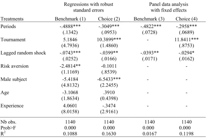
The descriptive statistics shown above refer to averages. Next, we account for individual characteristics. In Table 3, regressions (1) and (2) give the results of OLS regressions of the effort decisions in each treatment, with robust standard errors and accounting for clustering of the individuals; regressions (3) and (4) use panel data analysis with fixed effects. Explanatory variables include a time trend to capture learning, the mode of payment to capture the impact of competition, the random shock in the previous period and a series of individual characteristics such as gender, age, experience of experiments, and the degree of risk aversion. The risk aversion variable (coded from 1 to 10) corresponds to the number of the decision where the subject crosses over from the safer to the riskier option in the lottery test: the higher this number, the more risk averse the subject.

The main differences between the two treatments are related to the influence of the mode of payment and of risk aversion. In the Benchmark Treatment, the subjects do not exert a significantly higher effort in tournaments than under a piece-rate scheme. In contrast, competition stimulates performance when the subjects self-select, possibly because they consider that being volunteers, their opponents are also willing to compete hard. Risk aversion has a significant negative impact on effort when the payment schemes are imposed on the subjects: considering the uncertainty of the environment, risk-averse subjects reduce their cost. This variable is not significant in the Choice Treatment, suggesting that risk aversion plays a

role in the sorting process, but not once the choice has been made. The reverse is true for gender. In both treatments effort declines over time but this tendency is less pronounced when the subjects are allowed to choose their scheme. Although the periods are independent, the subjects in both treatments adjust their effort downwards (upwards) when they have got a positive (negative) random shock in the previous period.

Table 3. Determinants of the effort decision

Regressions with robust standard errors

Panel data analysis with fixed effects Treatments Benchmark (1) Choice (2) Benchmark (3) Choice (4) Periods

Tournament

Lagged random shock

Risk aversion Male subject Age Experience -.4888*** (.1342) 5.1846 (4.7936) -.0743*** (.0252) -2.4814** (1.1169) -5.4184 (4.8132) -3.1068 (1.8634) 4.0601 (8.0158) -.3049*** (.0953) 10.3899*** (1.4860) -.0399** (.0166) -0.1011 (.8539) -6.5433*** (2.2455) .3910 (0.4398) -.3474 (2.9161) -.4822*** (.0728) - -.0393** (.0171) - - - - -.2958*** (.0689) 11.8411*** (.8753) -.0294* (.0162) - - - - Nb obs. Prob>F R2 1140 0.000 0.1088 1140 0.000 0.1630 1140 0.000 0.0167 1140 0.000 0.1198 Note: Standard errors in parentheses; *** significant at 1% level, ** at 5% level, * at the 10% level.

The third and fourth columns of Table 3 display the estimations accounting for the longitudinal character of the data and including individual fixed effects. We may note that the coefficients to the lagged random shock are reduced but continue to differ from zero, whereas the other coefficients do not change much. In particular, it is worth remarking that the estimate to the tournament dummy in the choice treatment is larger, not smaller, when fixed effects are

entered. This is interesting because the fixed effects, in addition to the individual characteristics included in columns 1 and 2, are also picking up the impact of time-invariant unobservables.

Behavior in the Choice Treatment clearly differs from behavior in the Benchmark Treatment. It is therefore important to understand what determines sorting.

4.2. Sorting

In the Choice Treatment, the competitive scheme is chosen in 50% of the cases. Its relative frequency declines slightly from 52.7% in the first ten periods to 47.3% in the subsequent ten periods. This corresponds to the theoretical prediction since the expected utility in the tournament and the piece-rate scheme is the same. Does it mean that subjects choose at random or can we identify subjects’ characteristics that predict their behavior?

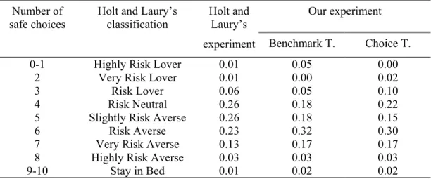
A first candidate for a determinant of sorting is risk aversion. Table 4 compares the distribution of our subjects in terms of risk attitude to the results in Holt and Laury (2002). Table 4. Distribution of risk attitudes

Our experiment Number of

safe choices

Holt and Laury’s classification

Holt and Laury’s

experiment Benchmark T. Choice T.

0-1 Highly Risk Lover 0.01 0.05 0.00

2 Very Risk Lover 0.01 0.00 0.02

3 Risk Lover 0.06 0.05 0.10

4 Risk Neutral 0.26 0.18 0.22

5 Slightly Risk Averse 0.26 0.18 0.15

6 Risk Averse 0.23 0.32 0.30

7 Very Risk Averse 0.13 0.17 0.17

8 Highly Risk Averse 0.03 0.03 0.03

9-10 Stay in Bed 0.01 0.02 0.02

Note: The number of safe choices corresponds to the number of the decisions with the “safe” option A, and thus corresponds to the “risk aversion” variable in our econometric analysis.

We observe higher proportions of risk lovers and more than slightly risk averse subjects than in Holt and Laury’s pool of subjects, but the differences are small. A Kolmogorov-Smirnov exact test does not reject the hypothesis of equality of distribution functions between our Benchmark and Choice Treatments.

Figure 3 relates the frequency of our subjects’ tournament choices to their proportion of safe choices in the ten decisions of the lottery task. Contestants have been grouped into three categories: subjects who choose the tournament in at least 14 periods out of 20 (“tournament

+”), subjects who choose the tournament in 6 periods or less (“tournament -“), and an

intermediate category (“tournament =”). The dashed line corresponds to the behavior of a risk neutral agent switching from option A to option B at decision 5.

0% 20% 40% 60% 80% 100%

Dec1 Dec2 Dec3 Dec4 Dec5 Dec6 Dec7 Dec8 Dec9 Dec10

Tournament + Tournament = Tournament Average -Choice Treatment

Fig.3. Proportion of safe lottery choices and frequency of the tournament choices

Clearly, the subjects who choose the tournament less frequently are more risk averse than the other categories.9 All risk-averse subjects considered together (who made at least 5 safe lottery

9

We checked that although made at the end of the sessions, the lottery decisions do not result from the behavior in the main game instead of explaining it. In fact, there is no correlation between the number of safe choices in the lotteries and the individual’s net payoff.

choices) choose the tournament in 45% of the periods, whereas the corresponding proportions are 60% for the risk neutral subjects and 56% for the risk lovers. A Poisson count model of the total number of tournaments chosen by the subject throughout the session has been estimated, including individual characteristics. It shows that only risk aversion exerts a significant influence and its marginal effect is important: crossing over from the safer to the riskier option one decision later in the lottery choices reduces by 77.8% the number of tournament choices. We have also conducted an econometric analysis of the choice of the tournament scheme, the results of which are reported in Table 5. Regression (1) estimates a panel probit model with random effects, and regression (2) a panel logit model with fixed effects.10

Table 5. Determinants of the tournament choice

Panel Probit model, with random effects (1)

Panel Logit model with fixed effects (2) Periods

Lagged random shock

Risk aversion Male subject Age Experience Constant -.0173** (.0074) -.0030* (.0017) -.1461** (.0745) -.0227 (.2176) -.0349 (.0355) -.0923 (.2564) 1.7981** (.8511) -.0295** (.0125) -.0051* (.0029) Nb observations Wald χ2 / LR χ2 Prob>χ2 Log Likelihood 1140 14.61 0.023 -691.00 1102 8.60 0.014 -517.07 Note: standard errors in parentheses; ** significant at 5% level, * at 10% level.

10

We also tested a selection model with random effects, including the treatment variable in the non-selection equation, fitted by simulated maximum likelihood. The selection equation included risk aversion, demographic variables and lagged random shock. The results are consistent with Table 3 and 4, except that gender looses its significance. However, the robustness of this selection model is not big because of the small number of variables, especially time-varying ones.

This analysis confirms that the degree of risk aversion is an important determinant of the choice of the competitive scheme, whereas demographic characteristics exert no effect.

The tournament choice is also affected by previous outcomes. The regression shows that it declines over time and that bad luck in the previous period increases the probability to enter the competition. This may reflect the subjects’ attempts to get the winner’s prize to compensate for small earnings in the previous period. Lastly, descriptive statistics indicate that if 70% of those who won a tournament in the previous period choose to remain in the competitive scheme, this percentage decreases to 55% among those who lost the previous competition.

Overall, these results suggest that risk aversion may be an important determinant of occupational choices. They are consistent with the survey analysis by Bonin et al. (2006) carried out on German data, which shows that risk averse employees tend to concentrate in jobs with low earnings risks.

4.3 Heterogeneity of Behavior in Tournaments

To investigate the behavioral origins of the reduction of effort variability when individuals self-select into tournaments, we adopt a cluster analysis that helps in identifying different types of behavior. In order to partition the sample, we retain three variables that summarize each individual’s decisions: her frequency of tournament choices, her mean effort in the tournament and its standard deviation. In the Benchmark treatment, we only consider the last two variables. We apply the hierarchical Wald method based on the minimization of the intra-group varianceto identify the clusters that sum up the strategies. Clusters have been grouped so that each one includes at least 10% of the subjects.

In both treatments, four main categories of tournament players are identified displaying similar characteristics; therefore we use the same denomination of clusters. The so-called “underconfident competitors” are subjects who exert an excessively high level of effort (more than 50% above the equilibrium), with relatively low standard deviation. The “motivated

competitors” are subjects who exert a level of effort still higher than the equilibrium but closer

to it. The “hesitant competitors” group consists of subjects who alternate levels of effort below and above the equilibrium and are characterized by the highest standard deviation of effort. Lastly, “economizing competitors” are subjects who follow a stable strategy based on the choice of a level of effort below the equilibrium.

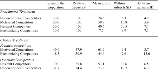
Table 6 summarizes the statistics that characterize these behaviors in each treatment. The first column indicates the proportion of each cluster in the population. The second column represents the relative frequency with which the tournament has been played during the session. The following columns give the mean individual effort and within-individual standard deviation of effort in the tournament. The last column gives the between-subject standard deviation within each cluster.

Table 6. Behavior in tournaments

Share in the population

Relative frequency

Mean effort Within-subjects SD Between-subjects SD Benchmark Treatment Underconfident Competitors 30.0 100 74.5 6.3 4.2 Motivated Competitors 30.0 100 59.9 10.8 5.4 Hesitant Competitors 30.0 100 40.6 20.5 7.1 Economizing Competitors 10.0 100 7.6 9.9 7.1 Choice Treatment Frequent competitors Motivated Competitors 40.0 57.9 61.9 9.4 3.7 Economizing Competitors 18.3 50.9 44.6 7.6 15.6 Occasional competitors Hesitant Competitors 10.0 35.8 53.1 32.6 6.5 Underconfident Competitors 31.7 34.4 73.2 10.7 6.3

In the Choice Treatment, the analysis identifies two main categories of subjects according to their frequency of tournament choice. Frequent competitors, who compete in at least half of the periods, are characterized by a lower within-subject variance of effort than the occasional competitors, who choose the tournament in about one third of the periods.

When they can select their payment scheme, the individuals who enter more frequently into the tournament are both the motivated and the economizing competitors. The group of motivated competitors is very homogenous as indicated by the low between-subject deviation. The relative importance of this group (40% of all the subjects involved in this treatment) contributes to explain the lower variance of effort in tournaments when individuals can self-select. In contrast, the group of economizing competitors shows the lowest within-subject and the highest between-subject variance of effort. It includes subjects who choose a minimum cost but can expect to win the tournament by chance. It also includes subjects who exert a level of effort slightly below equilibrium, possibly due to overconfidence or perception biases with respect to uncertainty, such as misconceptions of chance (Kahneman, Slovic, and Tversky 1982) or illusion of control over external events originated in being given a choice (Langer 1975).11 Whatever the explanation, their low-cost choices enable them to earn more on average than the motivated competitors (45.8 and 42.7, respectively).

The hesitant and the under-confident subjects are occasional competitors. The high within-subject variance of effort of the first group suggests that, facing the strategic uncertainty

11

In the first period of the game, after the subjects have chosen their level of effort, we asked them: « How big do you estimate your chances are that you will draw a random number that increases your payoff ? ». 14% reported a probability lower than .49 and 13% a probability exceeding .50. 61% of the optimistic subjects opted for the tournament, whereas the corresponding percentages are 47% for the pessimistic and 48% for the well-calibrated subjects. According to a probit regression (not shown) including only the first period data and individual observable characteristics, optimism marginally but significantly (at the 10% level) increases tournament entry. If all periods are considered, miscalibration is no longer significant since subjective beliefs are revised throughout the game.

attached to the tournament, these subjects make errors both above and below the equilibrium. Entering the tournament less often reinforces the difficulties of learning the equilibrium. Consequently, they earn less on average in the tournament than the frequent competitors (40.8 points). The group of under-confident competitors is also not able to compute the equilibrium but always exerts a very high level of average effort in tournaments (73.2, i.e. 52.5% above the equilibrium). As a consequence, even if they win relatively often the competition, the cost of effort is too high and thus they earn considerably less on average than under the piece-rate scheme (36 and 50.6 points, respectively).

The comparison between treatments indicates that the reduction of the effort variability in tournaments when agents can self-select is due to the fact that the most extreme categories in terms of average effort and the most unstable agents tend to stay out of the competition. The experiment points to a potential limitation of sorting. The motivated competitors provide an over-supply of effort and their net earnings are not very high. These subjects do not enter into a rat race (effort does not increase over time), but nevertheless, sorting reinforces a tendency to exert excess effort from some employees.

5. Discussion and Conclusion

In a one-shot game environment, our results confirm that both the average level and the variance of effort are higher under a tournament than under a piece-rate payment scheme. This higher variability of effort has long been considered an important disadvantage since the employers have to bear uncertainty as to how the agents behave in relative performance compensation schemes. However, by analyzing an experimental setting which accounts for a key feature of markets, that the agents can choose their payment scheme, our results paint a fundamentally different picture. A major finding of this paper is that when the subjects enter

the tournament voluntarily, the average effort is higher and the variance of effort is substantially lower compared to situations in which the same payment scheme is imposed. In our experiment, average effort in the freely chosen tournament is 32.5% higher than in the exogenously imposed piece-rate scheme. This differential can be decomposed into an incentive and a sorting effect. The difference between effort levels in the imposed piece-rate and in the imposed tournament is an estimate of the incentive effect of tournaments: here, this is of the magnitude of a 14.6% increase in effort. The difference of 17.9% between the total increase in effort and the estimated incentive effect can be attributed to the sorting effect of tournaments. The sorting effect makes up a little more than half of the total increase in effort; this is comparable to Lazear’s (2000) corresponding estimates in connection with the switch from a fixed pay to a variable pay scheme. This confirms the importance of taking sorting into account when evaluating the efficiency of compensation schemes.

Another important and new result is that sorting significantly decreases the variance of effort in tournaments. When agents freely enter the tournament, the between-subject variance is four times smaller than when this scheme is imposed and it is even lower than the variance of effort under the piece-rate scheme. It is worth noting that we obtain this result in spite of the increased complexity of the task to be performed as compared with previous studies. Consequently, our experiment does not lead to the same recommendations as Bull, Weigelt and Schotter (1987), who suggest that to attract contestants, an employer should offer them a higher expected utility than under a piece-rate scheme. Our conclusion is rather that labor market flexibility, in particular the absence of restrictions on mobility between firms, is a key condition for a higher efficiency of relative performance pay.

Our results indicate that the efficiency-enhancing effect of sorting derives from the resulting greater homogeneity of contestants. Since tournaments involve higher uncertainty than the piece-rate scheme, risk averse subjects choose them to a lesser extent. Under-confident subjects also prefer the piece-rate scheme since they exert too much effort in the tournament, entailing an excessive cost of effort. Hesitant subjects, alternating between above and below equilibrium effort levels, are not attracted by the tournament either. On the other hand, individuals who are motivated to work hard do not hesitate to choose the tournament in which equilibrium effort is higher. Among frequent contestants, the motivated competitors represent the biggest and the most stable category. Thus, the homogeneity of the contestants is higher when the tournament is chosen and this contributes to the lower variance of effort. More homogeneity does not, however, give rise to collusion. Beyond this, our results suggest that introducing more competitive payment schemes in some occupations would sort employees and that the attitude toward risk may be an important driver of mobility between firms or sectors.

Having demonstrated that sorting has profound implications for the level and variance of effort in tournaments, we think further work should focus on how sorting is affected both by the prize structure and by differences in individuals’ skills and social preferences: if people care about the negative externalities imposed on others by their individual effort, they may try not only to reduce their level of effort in relative pay scheme (Bandiera, Barankay, and Rasul 2005), but also to stay out of a competition. Our work suggests more generally the importance of reconsidering the influence of sorting in many economic decisions.

Appendix. Instructions of the Choice Treatment

You are about to participate in an experiment on decision-making organized for the GATE research institute and the Aarhus School of Business in Denmark. During this session, you can earn money. The amount of your earnings depends on your decisions and on the decisions of the participants you will have interacted with. During the session, your earnings will be calculated in points,

with 80 points = 1Euro

During the session, losses are possible. However, they can be avoided with certainty by your decisions. In addition, if a loss would occur in a period, the gains realized during the other periods should compensate this loss. At the end of the session, all the profits you have made in each period will be added up and converted into Euros. In addition, you will receive a show-up fee of 3 Euros. You will have also an opportunity to earn additional money by participating in a decision task at the end of the session. Your earnings will be paid to you in cash in a separate room in order to preserve confidentiality.

The session consists of 20 independent periods.

___________

Description of each period

Each period consists of two stages.

In stage 1, you choose between two modes of payment, mode X and mode Y. In stage 2, you carry out a task.

Your profit during each period depends on the mode of payment you have chosen and on your result from the task.

Description of the task

o _{A table is attached to these instructions: numbers, from 0 to 100, are given in column A. In the second stage} of each period, your task consists of selecting one of these numbers. This number will be called your “decision number”. Associated with each number is a cost, called “decision cost”. These decision costs are listed in column B. Note that the higher the decision number chosen, the greater is the associated cost. You make your choice by means of a scrollbar on your computer screen and you confirm this choice by clicking the “OK” button.

o _{Then, you have to click a button on your screen that will generate a random number. This number is called} your “personal random draw number”. This number can take any value between – 40 and + 40. Each number between – 40 and + 40 is as likely to be drawn and there is one independent random draw between – 40 and + 40 for each subject in the lab.

Your “result” for the task is the sum of your decision number and your personal random draw number. Your result = your decision number + your personal random draw number

Choice of the mode of payment and calculation of your payoff

There are two different modes of payment, mode X and mode Y. In the first stage of each period, you choose to be paid according to mode X or to mode Y. If you like, you can change the mode of payment at each new period.

Description of mode of payment X

If you choose the mode of payment X, your result is multiplied by 0.52. You also receive a fixed amount of 45 points. Next, the decision cost associated to the choice of your decision number is subtracted. Note, the amount subtracted (your decision cost) is only a function of your decision number; that is, your personal random draw number does not affect the amount subtracted.

Your payoff thus depends on your decision number and your personal random draw number. Your net payoff under mode X is thus given by the following formula:

Your net payoff of the period under mode X = 45 + (your result * 0.52) – your decision cost

At the end of the period, you are informed about your result and about your net payoff for the current period.

Example of net payoff calculation under mode of payment X

For example, say that you choose a decision number of 55 and you draw a personal random number of 10. Your net payoff calculation will look like:

45 + [(55 + 10) * 0.52] – 20.17 = 58.63 Description of mode of payment Y

If you choose the mode of payment Y, another subject in the room, who has also chosen the mode of payment Y, is paired with you at random for the current period. This subject is called your “pair member”. The identity of your pair member will never be revealed to you.

Your pair member has an identical sheet as yours. Like you and simultaneously, he has to select a decision number and he will draw his personal random number. As for you, the “result” of your pair member is computed by adding his decision number and his personal random draw number.

Then, the computer program will compare your result and the result of your pair member.

- If your result is greater than your pair member’s result, you receive the fixed payment M, equal to 96 points.

- If your result is lower than your pair member’s result, you receive the fixed payment L, equal to 45 points.

- In case of equal results, a fair random move decides on which subject receives M and who receives L. Whether you receive M or L as your fixed payment depends only on whether your result is greater or not than your pair member’s. It does not depend on how much bigger it is.

To determine your net payoff, the decision cost associated with the choice of your decision number is subtracted. Note, the amount subtracted is only a function of your decision number; that is, your personal random draw number does not affect the amount subtracted.

Therefore, your net payoff depends on your decision number, your personal random draw number, and your pair member’s decision number and his personal random draw number.

Your net payoff under mode Y is given by the following formula:

Your net payoff of the period under mode of payment Y = Fixed payment (M or L) – your decision cost

At the end of the period, you are informed about your result; you are told by how much your total is greater or less than that of your pair member and you are informed about your net payoff for the current period.

Example of net payoff calculation under mode of payment Y

For example, say that pair member A chooses a decision number of 25 and draws a personal random number of 20, while pair member B selects a decision number of 55 and draws a personal random number of -5.

A’s result is: 25 + 20= 45 B’s result is: 55 - 5= 50

B’s result is larger than A’s result. Thus, B receives M (=96) and A receives L (=45). A’s net payoff is: 45 – 4.17 = 40.83

B’s net payoff is: 96 – 20.17 = 75.83

To sum up, in each period you make two decisions:

- In stage 1, you choose between mode of payment X and mode of payment Y. Note that if an uneven number of participants has chosen mode Y, one of these participants will be randomly chosen and paid according to mode X. To be paid according to mode Y, pairs must be formed. This participant will be informed of this before moving to stage 2.

- In stage 2, you select your decision number and you draw a personal random number. Your net payoffs for the current period are then computed.

At the end of a period, a new period starts automatically. Each period is independent. The random draws are independent from one period to the next. In each period, under mode of payment Y, pairs are composed at random among the participants who have chosen this mode of payment.

---

If you have any question regarding these instructions, please raise your hand. Your questions will be answered in private. Throughout the entire session, talking is not allowed. Any violation of this rule will result in being excluded from the session and not receiving payment.

Decision Costs Table Column A Decision Nb Column B Cost of Decision Column A Decision Nb Column B Cost of Decision Column A Decision Nb Column B Cost of Decision 0 0.00 35 8.17 70 32.67 1 0.01 36 8.64 71 33.61 2 0.03 37 9.13 72 34.56 3 0.06 38 9.63 73 35.53 4 0 .11 39 10.14 74 36.51 5 0.17 40 10.67 75 37.50 6 0.24 41 11.21 76 38.51 7 0.33 42 11.76 77 39.53 8 0.43 43 12.33 78 40.56 9 0.54 44 12.91 79 41.61 10 0.67 45 13.50 80 42.67 11 0.81 46 14.11 81 43.74 12 0.96 47 14.73 82 44.83 13 1.13 48 15.36 83 45.93 14 1.31 49 16.01 84 47.04 15 1.50 50 16.67 85 48.17 16 1.71 51 17.34 86 49.31 17 1.93 52 18.03 87 50.46 18 2.16 53 18.73 88 51.63 19 2.41 54 19.44 89 52.81 20 2.67 55 20.17 90 54.00 21 2.94 56 20.91 91 55.21 22 3.23 57 21.66 92 56.43 23 3.53 58 22.43 93 57.66 24 3.84 59 23.21 94 58.91 25 4.17 60 24.00 95 60.17 26 4.51 61 24.81 96 61.44 27 4.86 62 25.63 97 62.73 28 5.23 63 26.46 98 64.03 29 5.61 64 27.31 99 65.34 30 6.00 65 28.17 100 66,67 31 6.41 66 29.04 32 6.83 67 29.93 33 7.26 68 30.83 34 7.71 69 31.74

Post experimental questionnaire

[Instructions for the test of risk aversion directly taken from Holt and Laury, 2002 ]

We thank you for filling out this form that enables you to earn additional money. The attached sheet of paper shows ten decisions. Each decision is a paired choice between “Option A” and “Option B”. You will make ten choices and record these in the column on the right, but only one of them will be used in the end to determine your additional earnings. Let us explain how these choices will affect your earnings.

Here is a ten-sided die that will be used to determine this payoff. The faces are numbered from 1 to 10 (the “0” face of the die will serve as 10). After you have made all of your choices, and when you come to the other office to receive your payment, you will throw this die twice:

- once to select one of the ten decisions to be used,

- and a second time to determine what your payoff is for the option you chose, A or B, for the particular decision selected.

Even though we ask you to make ten decisions, only one of these will end up affecting your earnings. However, you will not know in advance which decision will be used. Obviously, each decision has an equal chance of being used in the end.

• Look at Decision 1.

Option A pays 2 € if the throw of the dice is 1, and it pays 1.6 € if the throw is 2-10. Option B yields 3.85 € if the throw of the dice is 1 and it pays 0.1 € if the throw is 2-10.

• Look at Decision 2.

Option A pays 2 € if the throw of the dice is 1 or 2, and it pays 1.6 € if the throw is 3-10. Option B yields 3.85 € if the throw of the dice is 1 or 2 and it pays 0.1 € if the throw is 3-10.

The other decisions are similar, except that as you move down the table, the chances of a higher payoff for each option increase. In fact, for Decision 10 in the bottom row, the dice will not be needed since each option pays the highest payoff for sure, so your choice here is between 2 € and 3.85 €.

To summarize,

- you will make ten choices. For each decision row, you will have to choose between Option A and Option B. You may choose A for some decision rows and B for other rows. You may change your decisions and make them in any order.

- When you come to the other room to receive your earnings from the experiment, you will throw the ten-sided die to select which of the ten decisions will be used.

- Then, you will throw the die again to determine your money earnings for the Option you chose for that Decision.

Earnings (in Euros) for this choice will be added to your previous earnings, and you will be paid all earnings in cash.

If you have any question, please raise your hand. Your questions will be answered in private. Please do not talk with anyone.

Please indicate for each of the following 10 decisions if you choose Option A or Option B. Your decision Decision 1 Option A: 1/10 of 2 € and 9/10 of 1.6 € Option B: 1/10 of 3.85 € and 9/10 of 0.1 € Option A O Option B O Decision 2 Option A: 2/10 of 2 € and 8/10 of 1.6 € Option B: 2/10 of 3.85 € and 8/10 of 0.1 € Option A O Option B O Decision 3 Option A: 3/10 of 2 € and 7/10 of 1.6 € Option B: 3/10 of 3.85 € and 7/10 of 0.1 € Option A O Option B O Decision 4 Option A: 4/10 of 2 € and 6/10 of 1.6 € Option B: 4/10 of 3.85 € and 6/10 of 0.1 € Option A O Option B O Decision 5 Option A: 5/10 of 2 € and 5/10 of 1.6 € Option B: 5/10 of 3.85 € and 5/10 of 0.1 € Option A O Option B O Decision 6 Option A: 6/10 of 2 € and 4/10 of 1.6 € Option B: 6/10 of 3.85 € and 4/10 of 0.1 € Option A O Option B O Decision 7 Option A: 7/10 of 2 € and 3/10 of 1.6 € Option B: 7/10 of 3.85 € and 3/10 of 0.1 € Option A O Option B O Decision 8 Option A: 8/10 of 2 € and 2/10 of 1.6 € Option B: 8/10 of 3.85 € and 2/10 of 0.1 € Option A O Option B O Decision 9 Option A: 9/10 of 2 € and 1/10 of 1.6 € Option B: 9/10 of 3.85 € and 1/10 of 0.1 € Option A O Option B O Decision 10 Option A: 10/10 of 2 € and 0/10 of 1.6 € Option B: 10/10 of 3.85 € and 0/10 of 0.1 € Option A O Option B O

References

Bandiera, Oriana; Barankay, Iwan and Rasul, Imran, (2005). "Social Preferences and the Response to Incentives: Evidence from Personnel Data." Quarterly Journal of

Economics, 120(3), 917-62.

Bognanno, Michael L., (2001). "Corporate Tournaments." Journal of Labor Economics, 19(2), 290-315.

Bohnet, Iris and Kübler, Dorothea, (2004). "Compensating the Cooperators: Is Sorting in the Prisoner's Dilemma Game Possible?" Working Paper.

Bonin, Holger; Dohmen, Thomas; Falk, Armin; Huffman, David and Sunde, Uwe, (2006). "Cross-Sectional Earnings Risk and Occupational Sorting: The Role of Risk Attitude."

IZA Discussion Paper, 1930. Bonn.

Bull, Clive; Schotter, Andrew and Weigelt, Keith, (1987). "Tournaments and Piece-Rates: An Experimental Study." Journal of Political Economy, 95(1), 1-33.

Cadsby, C. Bram; Song, Fei and Tapon, Francis, (2004). "The Effects of Compensation Schemes on Self-Selection and Productivity: An Experimental Investigation." Working

Paper.

Datta Gupta, Nabanita; Poulsen, Anders and Villeval, Marie-Claire, (2005). "Male and Female Competitive Behavior -Experimental Evidence." IZA Discussion Paper, 1833. Bonn. Dohmen, Thomas and Falk, Armin, (2005). "Sorting, Incentives and Performance." , IZA

working paper, Bonn.

Ehrenberg, Ronald G. and Bognanno, Michael L., (1990a). "Do Tournaments Have Incentive Effects?" Journal of Political Economy, 98(6), 1307-24.

____, (1990b). "The Incentive Effects of Tournaments Revisited: Evidence from the European Pga Tour." Industrial and Labor Relations Review, 43(3), 74S-88S.

Eriksson, Tor, (1999). "Executive Compensation and Tournament Theory: Empirical Tests on Danish Data." Journal of Labor Economics, 17(2), 262-80.

Eriksson, Tor and Villeval, Marie-Claire, (2004). "Other-Regarding Preferences and Performance Pay: An Experiment on Incentives and Sorting." IZA Discussion Paper, 1191. Bonn.

Fershtman, Chaim and Gneezy, Uri, (2004). "Quitting." Tel-Aviv University, Mimeo.

Fullerton, Richard L. and McAfee, R. Preston, (1999). "Auctioning Entry into Tournaments."

Journal of Political Economy, 107(3), 573-605.

Green, Jerry R. and Stokey, Nancy L., (1983). "A Comparison of Tournaments and Contracts." Journal of Political Economy, 91, 349-64.

Harbring, Christine and Irlenbusch, Berndt, (2003). "An Experimental Study on Tournament Design." Labour Economics, 10, 443-64.

____, (2004). "Incentives in Tournaments with Endogenous Prize Selection." IZA Discussion

Paper, 1340. Bonn.

Holt, Charles A. and Laury, Susan K., (2002). "Risk Aversion and Incentive Effects."

American Economic Review, 92(5), 1644-55.

Hvide, Hans K. and Kristiansen, Eirik G., (2003). "Risk Taking in Selection Contests." Games