Nano-rheology at soft interfaces probed by atomic force microscope
122
0
0
Texte intégral
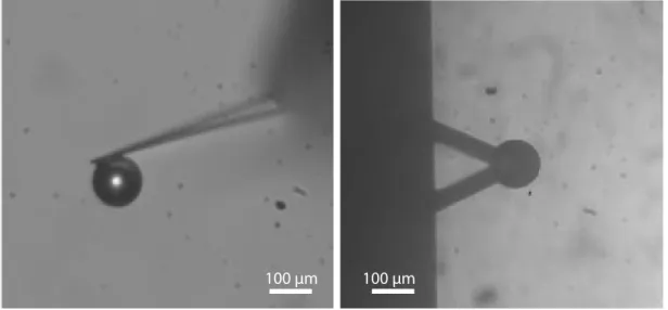
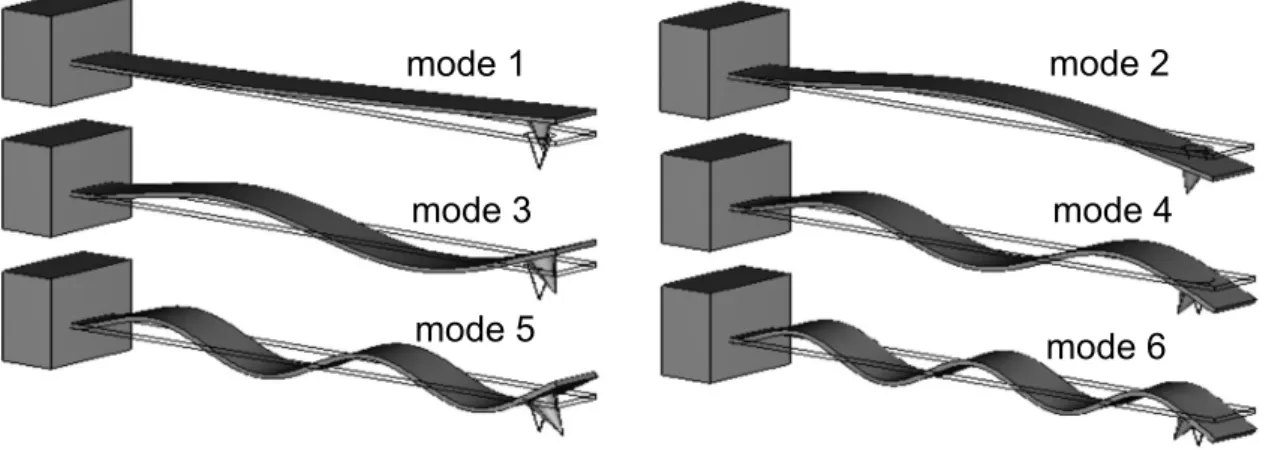
Figure


+7


Documents relatifs