Geometry and dynamics of configuration spaces

(1)

HAL Id: tel-01250817

https://tel.archives-ouvertes.fr/tel-01250817

Submitted on 5 Jan 2016

HAL is a multi-disciplinary open access archive for the deposit and dissemination of sci-entific research documents, whether they are pub-lished or not. The documents may come from teaching and research institutions in France or abroad, or from public or private research centers.

L’archive ouverte pluridisciplinaire HAL, est destinée au dépôt et à la diffusion de documents scientifiques de niveau recherche, publiés ou non, émanant des établissements d’enseignement et de recherche français ou étrangers, des laboratoires publics ou privés.

Mickaël Kourganoff

To cite this version:

Mickaël Kourganoff. Geometry and dynamics of configuration spaces. Differential Geometry [math.DG]. Ecole normale supérieure de lyon - ENS LYON, 2015. English. �NNT : 2015ENSL1049�. �tel-01250817�

(2)

Th`

ese

en vue de l’obtention du grade de

Docteur de l’Universit´

e de Lyon,

d´

elivr´

e par l’´

Ecole Normale Sup´

erieure de Lyon

Discipline : Math´ematiques

présentée et soutenue publiquement le 4 décembre 2015 par

Micka¨el Kourganoff

G´

eom´

etrie et dynamique des

espaces de conﬁguration

Directeur de th`ese : Abdelghani Zeghib

Devant la commission d’examen form´ee de :

Viviane Baladi (Universit´e Pierre et Marie Curie, Paris), examinatrice Thierry Barbot (Universit´e d’Avignon), rapporteur

G´erard Besson (Universit´e de Grenoble), examinateur ´

Etienne Ghys (´Ecole Normale Sup´erieure de Lyon), examinateur Boris Hasselblatt (Tufts University), rapporteur

Mark Pollicott (University of Warwick), rapporteur

Bruno Sévennec (École Normale Supérieure de Lyon), examinateur Abdelghani Zeghib (École Normale Supérieure de Lyon), directeur

(3)

(4)

Remerciements

Mes premiers remerciements vont à Ghani, qui m’a fait découvrir un sujet passionnant, riche et original, et m’a laissé une grande liberté, tout en sachant s’impliquer dans le détail dès que nécessaire. Merci aussi pour toutes ces heures passées dans ton bureau à m’expliquer avec patience et enthousiasme toutes ces mathématiques magnifiques.

Je suis très honoré que Thierry Barbot, Boris Hasselblatt et Mark Pollicott aient accepté d’être rapporteurs. Merci pour leur travail minutieux de relecture et leurs remarques qui ont contribué à améliorer ce manuscrit. Merci également à Viviane Baladi, Gérard Besson, Étienne Ghys et Bruno Sévennec d’avoir accepté de faire partie du jury. Merci à tous les membres de l’UMPA, et en particulier aux géomètres, toujours prêts à partager ce qu’ils savent, et qui ont toujours accepté mes invitations à parler au Séminaire Introductif Préparatoire Intelligible et Compréhensible (SIPIC) : Étienne, Ghani, Bruno, Jean-Claude, Damien, Olivier, Alexei, Emmanuel, Marco, Romain. . . Merci aussi à tous les thésards, post-docs ou AGPR grâce à qui l’ambiance est si agréable : Agathe, Alessandro, Alvaro, Anne, Arthur, Émeric, Fangzhou, Fran¸cois, Léo, Lo¨ıc, Marie, Marielle, Maxime, Michele, Olga, Rémi, Romain, Samuel, Sébastien, Valentin, Vincent, et tous les autres. Merci à Magalie et Virginia dont la gentillesse et l’efficacité ne sont plus à prouver. L’ENS Lyon est également un cadre privilégié pour débuter en tant qu’enseignant : merci à toute l’équipe enseignante, aux élèves, et à ceux qui ont préparé les TD avec moi et avec qui j’ai le plaisir d’échanger des idées et des exercices (Alexandre et Alexandre, Daniel, Mohamed et Sylvain).

Mais je dois aussi beaucoup aux membres de l’Institut Fourier à Grenoble, où j’ai passé beaucoup de temps durant la seconde moitié de ma thèse. Merci à Gérard Besson pour son accueil chaleureux, à Pierre Dehornoy pour avoir relu et aidé à améliorer un passage de ma thèse, et à Benoˆıt Kloeckner et Frédéric Faure pour des discussions fructueuses. Merci à Kévin et Simon qui ont partagé mon bureau à Grenoble et l’ont rendu vivant, mais aussi à Alejandro, Bruno, Clément, Guillaume, Simon, Thibaut et aux autres thésards grenoblois.

Merci à Daniel et à ma mère d’avoir corrigé un certain nombre de maladresses de mon anglais dans cette thèse.

Merci à Jos Leys, qui contribue bénévolement depuis des années à la recherche mathématique, en créant des images et des vidéos de grande qualité qui rendent les mathématiques plus concrètes et accessibles. Ce fut un grand plaisir de travailler avec lui : je lui dois toutes les images du chapitre8, ainsi qu’une vidéo qui illustre le résultat principal de ce chapitre.

Merci à Pierre Joly pour m’avoir transmis sa passion des maths il y a bien longtemps. Merci à ceux avec qui j’ai eu la chance de faire de la belle musique pour me changer les idées pendant ces années de thèse : les élèves et les profs des classes de chant et de

(5)

direction des conservatoires de Villeurbanne et Grenoble, les chanteurs de l’UMPA et du LIP avec qui j’ai découvert l’improvisation dans le style de la renaissance, les chanteurs d’Émelthée, les membres des chœurs que j’ai eu grand plaisir à diriger à Saint-Cyr au Mont d’Or et à Meylan, tous les musiciens intrigués par le métier de chercheur en mathématiques.

Merci aux membres du Raton-Laveur ou assimilés (Aisling, Aurore, Benjamin, Benoˆıt, Camille, Élodie, Guillaume, Guillaume, Hélène, Irène, Jonas, Marthe, Laetitia, Mikaël, Nathanaël, Ophélia, Pierre, Quentin, Rémi, Timothée et les autres) pour tous ces mails inutiles dont je ne pourrais pas me passer, pour ces randonnées, laser games, parties de Sporz, LANs de tetrinet ou concours de xjump. Merci à Martin, Margaret, Guillaume, Samuel, Solène, Clémence, et les autres qui ont égayé mes week-ends de retour à Paris. Merci à tous les membres de ma famille pour leur soutien, et pour m’avoir gentiment écouté leur expliquer en quoi le mécanisme de Peaucellier était une invention géniale.

Enfin, merci à Laetitia, pour sa relecture des pages de ma thèse qui contiennent le mot “graphe”, et surtout, pour tout le reste.

(6)

Introduction (fran¸cais)

Cette thèse est divisée en trois parties qui peuvent être lues indépendamment. Dans la première, on étudie les théorèmes d’universalité pour les mécanismes (aussi appelés systèmes articulés) dont l’espace ambiant est une surface homogène. Dans la seconde, on étudie un lien entre flots géodésiques et billards, ainsi que la dynamique de certains mécanismes. La troisième porte sur les structures de similitude transverses sur les feuilletages, ainsi que sur le théorème de décomposition de De Rham. Chacune de ces parties contient une introduction propre.

Un mécanisme est un ensemble de tiges rigides reliées par des liaisons pivots. Mathématiquement, on considère un mécanisme comme un graphe muni d’une structure supplémentaire : on associe une longueur à chaque arête (le graphe est dit métrique), et certains sommets sont fixés au plan tandis que d’autres évoluent librement. Une réalisation d’un mécanisme dans le plan est le choix d’une position dans le plan pour chaque sommet, de sorte que les longueurs associées aux arêtes correspondent aux distances dans le plan entre les sommets correspondants. En particulier, on autorise les arêtes à se croiser. Enfin, l’espace de configuration d’un système articulé est l’ensemble de ses réalisations.

Le premier chapitre constitue une introduction à cette notion de mécanisme : on y donne des éléments historiques, et des exemples fondamentaux, qui sont utiles pour les chapitres suivants.

La première partie, qui suit cette introduction, est constituée de quatre chapitres et correspond à la pré-publication [Kou14] : on y étudie des mécanismes dont l’espace ambiant n’est plus le plan, mais diverses variétés riemanniennes. Le chapitre 2introduit la question de l’universalité des mécanismes : cette notion correspond à l’idée que toute courbe serait tracée par un sommet d’un mécanisme, et que toute variété différentiable serait l’espace de configuration d’un mécanisme. On y présentera des résultats déjà connus qui vont dans ce sens pour les mécanismes dans le plan : d’une part, les courbes que l’on peut tracer sont exactement les courbes semi-algébriques compactes ; et d’autre part, pour toute variété compacte connexe M , il existe1 _{un espace de configuration d’un}

système articulé dont toutes les composantes connexes sont difféomorphes à M . Ce même chapitre contient aussi les énoncés de tous les nouveaux résultats essentiels de cette partie, qui consistent à étendre les théorèmes d’universalité au plan de Minkowski, au plan hyperbolique et enfin à la sphère. Dans chaque cas, les difficultés rencontrées diffèrent, ainsi que les techniques pour les résoudre, mais les résultats obtenus sont très similaires, sauf dans le cas du plan de Minkowski, où l’on s’affranchit de l’exigence de compacité : l’universalité est alors valable dans un sens encore plus large. Les trois derniers chapitres contiennent les démonstrations de ces énoncés, alors que les outils généraux sont donnés 1_{On ne sait toujours pas, cependant, si l’on peut exiger ou non que l’espace de configuration soit}

difféomorphe à la variété M elle-même.

(9)

dans le chapitre 2.

La seconde partie est constitu´ee de trois chapitres, dont les deux derniers correspondent `

a la pré-publication [Kou15a]. Dans le chapitre 6, on établit un premier lien entre flots géodésiques sur des variétés à courbure négative et billards dispersifs, en mettant en parallèle les comportements de ces deux systèmes. La similitude entre ces deux systèmes est bien connue depuis les travaux de Sina¨ı dans les années 1960, mais elle est rarement détaillée dans la littérature. Dans le même ordre d’idée, on donne une condition suffisante pour qu’un flot géodésique sur une surface fermée soit Anosov : il suffit que toutes les solutions de l’équation de Ricatti le long des géodésiques, nulles au temps t = 0, soient supérieures à une même constante m > 0 lorsque t = 1. Ce théorème bien connu a été utilisé à plusieurs reprises dans la littérature, mais sans qu’aucune preuve écrite ne semble disponible : nous l’utiliserons à notre tour dans les résultats qui suivent. Dans le chapitre 7, on présente deux résultats nouveaux concernant le flot géodésique de surfaces dans_R3 _{euclidien, qui ont subi une forte contraction selon l’un des axes. Toute}

surface dansR3 peut être aplatie selon l’axe des z, et la surface aplatie s’approche d’une table de billard dansR2. On montre que, sous certaines hypothèses, le flot géodésique de la surface converge localement uniformément vers le flot de billard. De plus, si le billard est dispersif, les propriétés chaotiques du billard remontent au flot géodésique : on montre qu’il est alors Anosov. Enfin, dans le chapitre 8, on donne des généralités sur la dynamique des systèmes articulés, puis on applique le résultat du chapitre 7à la théorie des systèmes articulés. Ceci permet d’obtenir un nouvel exemple de mécanisme Anosov, comportant cinq tiges. C’est la première fois qu’on exhibe un système articulé Anosov dont les longueurs des arêtes sont données explicitement. Une vidéo de ce mécanisme, due à Jos Leys, est disponible sur ma page web.

La troisième partie n’a pas de lien direct avec les deux autres, si ce n’est l’étude de variétés riemanniennes : elle correspond à la pré-publication [Kou15b]. On s’intéresse d’abord aux variétés munies de connexions localement métriques, c’est-à-dire de connexions qui sont localement des connexions de Levi-Civita de métriques riemanniennes ; on donne dans ce cadre un analogue du théorème de décomposition de De Rham, qui s’applique habituellement aux variétés riemanniennes. Dans le cas où une telle connexion préserve une structure conforme, on montre que cette décomposition comporte au plus deux facteurs ; de plus, lorsqu’il y a exactement deux facteurs, l’un des deux est l’espace euclidienRq. On répond ainsi à une question posée dans [MN15b]. L’étude des connexions localement métriques qui préservent une structure conforme est étroitement liée à celle des “structures de similitude” sur les variétés : ce sont les structures obtenues par quotient d’une variété riemannienne M par un sous-groupe de son groupe de similitudes Sim(M ). La démonstration des résultats de cette partie passe par l’étude des feuilletages munis d’une structure de similitude transverse. Sur ces feuilletages, on montre un résultat de rigidité qui peut être vu indépendamment des autres : ils sont soit transversalement plats, soit transversalement riemanniens. Remarquons que ces résultats sont valables dans le cas C∞, alors que de tels problèmes n’avaient été étudiés précédemment que dans le cas analytique.

(10)

Introduction (English)

This thesis is divided into three parts which may be read independently. In the ﬁrst one, we study universality theorems for linkages whose ambiant space is a homogeneous surface. In the second one, we study the link between geodesic ﬂows and billiards, as well as the dynamics of some linkages. The third one is about transverse similarity structures on foliations, and De Rham’s decomposition theorem. Each of these parts contains its own introduction.

A linkage is a set of rigid rods joined together by hinges. Mathematically, one considers a linkage as a graph with an additional structure: lengths are given to the edges (the graph is said to be metric), and some vertices are ﬁxed to the plane while the others move freely. A realization of a linkage in the plane is the choice of a position in the plane for each vertex, so that the edge lengths match with the distance in the plane between the corresponding vertices. In particular, one allows the edges to cross. Finally, the conﬁguration space of a linkage is the set of all its realizations.

The ﬁrst chapter is an introduction to the notion of linkage: we will present the historical background, and fundamental examples, which are useful for the next chapters.

The first part, after this introduction, is composed of four chapters and corresponds to the preprint [Kou14]: we study linkages whose ambiant space is no longer the plane, but various Riemannian manifolds. Chapter2 introduces the question of the universality of linkages: this notion corresponds to the idea that every curve would be traced out by a vertex of some linkage, and that any differentiable manifold would be the configuration space of some linkage. We shall present some results in this direction which are already known for planar linkages: on the one hand, the curves which may be traced out are exactly compact semi-algebraic curves; on the other hand, for any compact connected manifold M , there exists2 _{a configuration space of a linkage whose connected components}

are all diffeomorphic to M . The same chapter also contains the statements of all the main new results of this part, which are extensions of universality theorems to the Minkowski plane, the hyperbolic plane, and finally the sphere. In each case, one encounters different difficulties, and makes use of different techniques, but the results which are obtained are very similar, except in the Minkowski case, where the compacity hypothesis is no longer necessary: universality then becomes valid in a broader sense. The last three chapters contain the proofs of these statements, while the general tools are given in Chapter2.

The second part is composed of three chapters, where the last two correspond to the preprint [Kou15a]. In Chapter 6, we establish a first link between geodesic flows on negatively curved manifolds and dispersive billiards, by putting in parallel the behaviors of these two systems. It is well-known since Sinai’s work in the 1960’s that these two 2_{It is still unknown, however, whether it is possible to require that the configuration space be}

diﬀeomorphic to the manifold M itself.

(11)

systems are similar, but they are rarely studied together in the literature. In the same vein, we give a sufficient condition for a geodesic flow on a closed surface to be Anosov: it suffices that all solutions of the Ricatti equation along the geodesics, which equal zero at time t = 0, are greater than a single constant m > 0 at time t = 1. This well-known theorem has been used several times in the literature, but has apparently never been awarded any written proof: we will use it ourselves in the new results of this part. In Chapter 7, we present two new results concerning the geodesic flow of surfaces in the EuclideanR3, which undergo a strong contraction in one direction. Any surface inR3 can be flattened with respect to the z-axis, and the flattened surface gets close to a billiard table in R2_{. We show that, under some hypotheses, the geodesic flow of the surface}

converges locally uniformly to the billiard flow. Moreover, if the billiard is dispersing, the chaotic properties of the billiard also apply to the geodesic flow: we show that it is Anosov in this case. Finally, in Chapter 8, we give generalities on the dynamics of linkages, and then apply the result of Chapter7 to the theory of linkages. This provides a new example of Anosov linkage, made of 5 rods. It is the first time that one exhibits an Anosov linkage whose edge lengths are given explicitly. A video of this linkage, by Jos Leys, is available on my website.

The third part does not have a direct link with the two others, except for the study of Riemannian manifolds: it corresponds to the preprint [Kou15b]. We ﬁrst consider manifolds with locally metric connections, that is, connections which are locally Levi-Civita connections of Riemannian metrics; we give in this framework an analog of De Rham’s decomposition theorem, which usually applies to Riemannian manifolds. In the case such a connection also preserves a conformal structure, we show that this decomposition has at most two factors; moreover, when there are exactly two factors, one of them is the Euclidean spaceRq. Thus, we answer a question asked in [MN15b]. The study of locally metric connections which preserve a conformal structure is closely linked to “similarity structures” on manifolds: these are the structures obtained by the quotient of a Riemannian manifold M by a subgroup of its similarity group Sim(M ). The proofs of the results of this part use foliations with transverse similarity structures. On these foliations, we give a rigidity theorem of independant interest: they are either transversally ﬂat, or transversally Riemannian. Notice that these results are valid in the C∞ case, while such problems had only been studied in the analytic case previously.

(12)

Chapter 1

What is a linkage?

A mechanical linkage, or simply linkage, is a graph whose vertices are considered as rigid rods. Let us state precise mathematical deﬁnitions.

Deﬁnition 1.1. A planar linkage _{L is a graph (V, E) together with:} 1. A function l : E→ R≥0 (which gives the length of each edge);

2. A subset F _{⊆ V of ﬁxed vertices (represented by on the ﬁgures);}

3. A function φ0 : F → R2 which indicates where the vertices of F are ﬁxed.

Deﬁnition 1.2. LetL be a planar linkage, and consider the Euclidean distance δ in R2_.

A realization of a planar linkage_{L is a function φ : V → R}2 such that: 1. For each edge (v1v2)∈ E, δ(φ(v1), φ(v2)) = l(v1v2);

2. φ|F = φ0.

The conﬁguration space Conf(_{L) is the set of all realizations φ of L: it is naturally} a subset of (R2)n, where n is the number of vertices. It inherits the topology of the ambiant Euclidean space. Finally, the workspace of a vertex v _{∈ V is the set} {φ(v) | φ realization of L}.

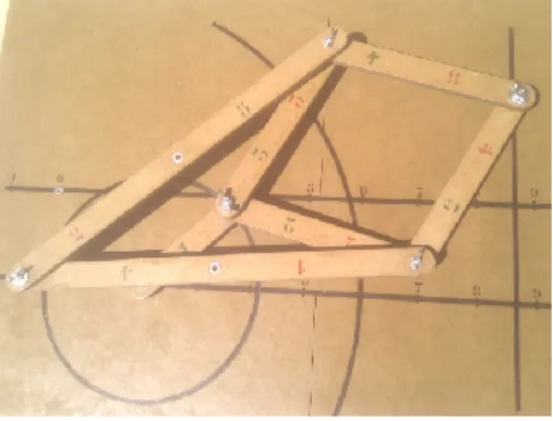
Figure 1.1 – A wooden realization of the Peaucellier straight-line motion linkage. Design: Adriane Ka¨ıchouh, Micka¨el Kourganoﬀ, Thomas Letendre. Construction: Pierre Gallais.

(13)

Linkages are one of the simplest physical examples involving manifolds of dimension 3 or more (other than the ambiant spaceR3): they appear naturally as configuration spaces. In Section1.1, we will give simple examples of linkages whose configuration space is diffeomorphic toTn_or_Sn_{, for any natural number n. Generically, the dimension of the}

conﬁguration space of a linkage is 2(|V | − |F |) − |E| (twice the number of free vertices, minus the number of edges). More precisely:

Proposition 1.3. Choose any graph (V, E), any F _{⊆ V and any φ}0 : F → R2. Then

there is a set L of full Lebesgue measure in RE such that for all choice of edge lengths l_{∈ L, the conﬁguration space of L = (V, E, l, F, φ}0) is a smooth orientable manifold of

dimension 2(_{|V | − |F |) − |E|.} Proof. Consider the function

F : (_R2)V\F _{→ R}E φ_{�→ f}φ

where, for any (vw)∈ E and any φ ∈ (R2₎V\F_,

fφ(vw) = δ(φ(v), φ(w))

(here, the domain of φ is extended to the whole V using φ0).

Then for any l∈ RE_{, the conﬁguration space of}_{L = (V, E, l, F, φ}

0) is F−1(l).

By Sard’s Theorem, the regular values of F form a set of full Lebesgue measure in RE_{. For such a value l, F}−1_{(l) is a smooth manifold of dimension 2(}_{|V | − |F |) − |E|.}

Moreover, sinceRE is orientable, the normal bundle of F−1(l) in (R2)V\F is orientable as well. But (R2)V\F itself is also orientable: one obtains an orientation of the tangent bundle of M , thus M is orientable.

Remark. Most of the linkages considered in Part I will not satisfy the assumptions of Proposition 1.3. In this case, the conﬁguration space may still be a smooth manifold, but it does not need to be orientable, and it is impossible to compute its dimension from the number of edges and vertices alone.

There exist many natural problems involving linkages, which cover various ﬁelds of mathematics, such as algebraic geometry, algebraic topology, Riemannian geometry, dynamical systems, and the theory of computational complexity. Many interesting problems involving complexity may be found in [DO07]. In this thesis, we focus on two particular aspects of linkages: universality and dynamics. The examples in the rest of this chapter are chosen in view of these two problems.

1.1 Fundamental examples

1.1.1 The robotic arm

The robotic arm _Rn (Figure 1.2) is a linkage whose underlying graph is a path (all

vertices have degree 2, except the two ends), with one ﬁxed end. It has n edges of lengths l1, l2, . . . , ln.

The conﬁguration space of _Rn is the torusTn: each of its conﬁgurations corresponds

(14)

1.1. FUNDAMENTAL EXAMPLES 13 v0 v1 v2 v3 l1 l2 l3 θ1 θ2 θ3

Figure 1.2 – The robotic arm _R3. Recall that ﬁxed vertices (here v0) are represented by

squares.

1.1.2 Polygons

A polygon is a linkage without ﬁxed vertices, whose underlying graph is a cycle.

It is often convenient to consider a polygon with two fixed adjacent vertices. In fact, fixing those two vertices amounts to removing the factor SO(2)� R2 which is found in the configuration space of any linkage without fixed vertices.

After fixing these two vertices at a distance which corresponds to the edge between them, one may remove this edge which has become useless, without changing the configuration space. Thus, a polygon may be seen as a robotic arm whose two ends are fixed.

Example.

a 1 1 1 1 1 1 1 1 b

Consider the linkage _Ln above with n edges. The vertices a and b are ﬁxed at a

distance n_{− � with a small enough � > 0, and all the edges have length 1.} Proposition 1.4. The conﬁguration space Conf(_Ln) is diﬀeomorphic to Sn−2.

Proof. We may assume that φ0(a) = (0, 0) and φ0(b) = (n− �, 0).

First, consider the robotic arm _Rn. For any conﬁguration (θ1, . . . , θn)∈ Conf(Rn),

write s = (s1, s2) = (�cos θi,�sin θi) ∈ R2 the position of the last vertex vn. Then

Conf(_Ln) ={(θ1, . . . , θn)∈ Tn | s = (n − �, 0)}: for a small � > 0, Conf(Ln) is contained

in an arbitrarily small neighborhood of _C0 = (0, . . . , 0).

Now, consider the subset of all conﬁgurations whose last vertex lies on the horizontal axis: E = _{{C ∈ T}n_{| s}2 = 0}. Since the gradient of s2 is ∇s2 =

   cos θ1 .. . cos θn   , E is a submanifold ofTn in a neighborhood ofC0.

Compute the diﬀerentials of s1 up to order 1 and 2:

∇s1 =−    sin θ1 .. . sin θn    and D2s1=−    cos θ1 0 . .. 0 cos θn    .

(15)

Thus, Ds1(C0) = 0 and D2s1(C0) is non-degenerate. Moreover, s1 reaches its global

maximum n atC0. With Morse’s Lemma, E is equipped with a global coordinate system

(xi)1≤i≤n−1 nearC0 such that:

s1− n = − �_n₋₁ � i=1 x2_i � .

In particular, the level of E deﬁned by s1 = n− � is diﬀeomorphic to a sphere of

dimension n_{− 2 for a small enough � > 0.}

This proof gives us a glimpse of how Morse theory may be used in view of determining the topology of some configuration spaces. The first chapter of [Far08] uses this approach to describe the homology groups of the configuration spaces of polygons.

1.1.3 Spider linkages

Although less famous than polygons, spider linkages (with n legs) provide interesting examples and were studied by many authors.

A spider is made of a central vertex to which n legs are attached, each of which has one articulation (each leg is a copy of_R2). The end of each leg is ﬁxed somewhere in the

plane. For n = 2, the spider is in fact a pentagonal linkage.

Since a spider has 2n edges and n + 1 free vertices, its conﬁguration space is a surface for a generic choice of the lengths of the edges: one may obtain a wide variety of surfaces in this way.

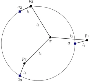
Spiders with n = 3. Thurston and Weeks [TW84] detailed a particular case of a spider with n = 3, which they called triple linkage (Figure 1.3).

a1 a2 a3 x p1 p2 p3 l1 l2 l1 l2 l1 l2

Figure 1.3 – Thurston and Weeks’ triple linkage. The three ﬁxed vertices are on the unit circle and form an equilateral triangle, and there are two length parameters l1 and l2.

In this case, each of the 3 legs of the spider restricts the movement of the central vertex to an annulus centered at ai, with inner radius|l1− l2| and outer radius l1+ l2.

(16)

1.1. FUNDAMENTAL EXAMPLES 15 Thus, the workspace of the central vertex is the intersection of three annuli. When the lengths l1 and l2 vary, this intersection may take diﬀerent shapes (Figure1.4).

Figure 1.4 – The workspace of the central vertex in Thurston’s triple linkage (in dark grey), for diﬀerent choices of the lengths.

Like Thurston and Weeks in their article, let us focus on the case1 _{on the left of}

Figure1.4: the workspace of the central vertex x is a hexagon. For each position of x in the interior of the hexagon, there are two possible positions for p1, which are symmetric

with respect to the line through x and a1. There are also two possible positions for

each of the two other vertices, so any point in the interior of the workspace of the central vertex corresponds to 8 points in the configuration space. The boundary of the hexagon corresponds to configurations in which at least one of the arms is completely stretched or folded. Such configurations belong in fact to several hexagons. Thus, the configuration space of the linkage is made of 8 copies of the hexagon, glued together along their boundaries. Each edge belongs to two hexagons, and each vertex to four hexagons, so the polyhedron has 8 faces, 24 edges and 12 vertices. Its Euler characteristic is 8− 24 + 12 = −4, so2 _{it is diffeomorphic to a surface of genus 3.}

For different choices of the edge lengths and positions of the fixed points, the inter-section of the three annuli may take many forms: in each case, it is possible to make a similar computation to determine the genus of the surface (for example, it is possible to obtain the disjoint union of 6 spheres, or a surface of genus 12). Ten different topologies for the configuration space of the triple linkage are given in [HM03].

The general case. In general, we have the following [Mou11]:

Theorem 1.5 (Mounoud, 2009). Let g be an natural number and r the biggest integer such that 2r _{divides g}_{− 1. A compact orientable surface of genus g is diﬀeomorphic to a}

spider’s conﬁguration space if and only if (1/2r)(g− 1) ≤ 6r + 12.

In particular, it is impossible to realize a surface of genus 14 as a conﬁguration space of a spider.

In 2006, O’Hara [O’H07] computed all the conﬁguration spaces obtained by a spider whose arms all have the same length length (l1= l2 = 1, with the notations of Figure1.3),

and whose ﬁxed vertices are on the unit circle and form a regular polygon P in R2_.

1_{This case corresponds, for example, to the condition (3/2}

− |l1− l2|)2+ 3/4 < (l1+ l2)2< (3/2 +

|l1− l2|)2+ 3/4 and|l1− l2| <√3/2.

2_{In fact, we should show ﬁrst that the conﬁguration space is a smooth orientable surface, which is}

not so obvious, even for generic lengths l1and l2. For example, one may compute directly the diﬀerential

(17)

Theorem 1.6 (O’Hara, 2006). Let R be the radius of the circumscribed circle to the poly-gonP. There exists a critical value Rn such that the conﬁguration space is diﬀeomorphic

to a connected orientable closed surface Σg if R satisﬁes:

0 < R < 2 and R�= Rn.

The genus g is given by g =

�

1− 2n−1_{+ n2}n−3_{+ n2}n−1_{= 1 + (5n}_{− 4)2}n−3 _{si 0 < R < R} n,

1_{− 2}n−1+ n2n−3 = 1 + (n_{− 4)2}n−3 si Rn< R < 2.

In his proof, O’Hara gives two methods to compute the genus: one of them is purely topological, while the other one uses Morse Theory. In the same paper, he also describes the singularities which appear when R does not satisfy the conditions of Theorem1.6.

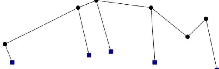
1.1.4 Centipedes

A centipede3 with n legs (Figure1.5) is a linkage whose underlying graph has 2n + 1 vertices, where n + 1 free vertices form a path, and n ﬁxed vertices are attached to the 1st_{, 2}nd_{, . . . , (n}_{− 1)}th _{and (n + 1)}th _{vertex of the path, as in the following ﬁgure:}

. . .

with any edge lengths, and any positions for the ﬁxed vertices.

Figure 1.5 – A centipede with 5 legs.

As for spiders, the conﬁguration spaces of centipedes are generically surfaces. It is remarkable that any connected closed oriented surface is the conﬁguration space of some centipede, as shown in [JS01].

In general, given a connected closed manifold M , it is unknown4 _{whether there exists}

a linkage whose conﬁguration space is diﬀeomorphic to M . This kind of problem is called “universality problem”: it is at the heart of PartI.

1.1.5 The pantograph

The pantograph (literally, a device which “writes everything” in Greek), invented by the astronomer Christoph Scheiner in 1603, was used to reproduce drawings at diﬀerent

3_{These linkages seem to have no standard name in the literature.} 4_{Even for connected closed non-orientable surfaces!}

(18)

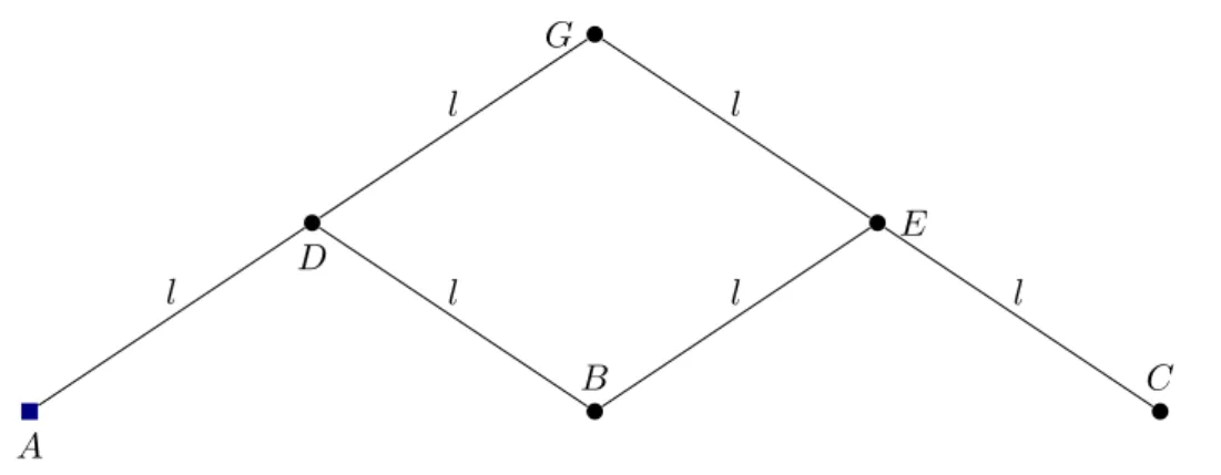
1.2. STRAIGHT-LINE MOTION 17 A G D B C E l l l l l l

Figure 1.6 – The pantograph. There is one rigid bar joining A (resp. C) to G, with a hinge D (resp. E) at the middle. The vertex A is ﬁxed.

scales (Figure1.6). The point C is the image of the point B by a homothety of center A and ratio 2. It is possible to obtain any other ratio by changing the edge lengths. In practice, a pen was ﬁxed to the vertex C and the vertex B was moved along the drawing which was to be copied. For this linkage (among others), we will be interested in the possible positions of the two vertices B and C, rather than the topology of the conﬁguration space.

Concerning the pantograph, two remarks are in order:

1. Here, we allowed some hinges (D and E) to be at the middle of bars, while our definition of a linkage as a mathematical graph requires them to be at the end. We could change the definition to include this situation, but in our setting, it is more convenient to consider AD and DG as two different edges of length l, as well as another edge of length 2l between A and G. The three vertices A, D, G form a flat triangle, so they are aligned for all configurations. With this technique, it is possible to add a hinge anywhere on a bar.

2. With our definitions, there are in fact many realizations of this linkage such that C is not the image of B by a homothety of center A. For example, for any position of A, C, G, there is a realization such that B = G. This is known as the problem of degenerated configurations: they have to be dealt with carefully when trying to understand the topology of configuration spaces. The same problem will occur in Section1.2.2. For more details, see [KM02] or Chapter 3.

1.2 Straight-line motion

The problem of straight-line motion appeared naturally when Watt designed his double-action steam engine in 1781. He needed a mechanism able to guide the piston of the engine along a straight line, and to transmit the energy to other elements of the system (for example, a wheel). With our deﬁnitions, the question was the following:

Question. Does there exist a linkage containing one vertex whose workspace is a line segment?

(19)

1 2 3 4 5

Figure 1.7 – Newcomen’s steam engine5. The cylinder (on the right) is ﬁlled with steam while the pump (on the left) is pulled down by its own weight (2). Then cold water is injected into the cylinder (3), which condensates the steam, creates vacuum and lowers the piston (4): at the other side, the pump goes up and takes the water out from the mine.

Earlier steam engines did not require such a mechanism. Half a century before Watt, Newcomen designed another steam engine, which was widely used to pump water from the coal mines. The steam only pulled the piston to one side (contrary to Watt’s double-action engine, where steam pulled it alternatively to both sides), and the mass of the pump on the other side pulled the piston back to its original position (Figure1.7). In Newcomen’s engine, it was possible to achieve straight-line motion with a simple ﬂexible chain. In contrast, Watt needed a rigid linkage to guide the piston.

1.2.1 Watt’s linkage

Watt’s linkage (Figure1.8) contains one vertex whose workspace is close to a straight line. It was used in Watt’s famous double-action steam engine, and is still used in the suspension systems of some cars.

For engineers, the problem of straight-line motion was solved, but for mathematicians, it was only the beginning.

Elementary computation shows that the workspace of the central vertex is the curve of equation (in polar coordinates):

r2 = b2− (a sin θ ±�c2_{− a}2_cos2_θ)2_.

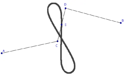
It is called Watt’s curve and, with a good choice of parameters, it has the shape of an eight (like on the ﬁgure). Near the center, it has curvature 0, so it is a straight line up to order 2, which is suﬃcient for most practical applications.

1.2.2 The Peaucellier inversor

In the 1860’s, Peaucellier and Lipkin discovered simultaneously a linkage which achieved perfect straight-line motion. First, we introduce the Peaucellier inversor (Figure1.9).

5_c

(20)

1.2. STRAIGHT-LINE MOTION 19

Figure 1.8 – Watt’s linkage (obtained with Geogebra), with the workspace of the central vertex E. It has two ﬁxed vertices A and B, and an additional vertex E at the middle of the edge CD. It is made of three bars AC, CD and DB: the bar CD has length 2c, while AC and DB have the same length length b. The distance between the ﬁxed vertices A and B is 2a. A D B C E l l l l r r

Figure 1.9 – The Peaucellier inversor. We assume that r > l.

Proposition 1.7. For any position of the Peaucellier linkage, the points A, D and E are aligned, and AD_{· AE = r}2_{− l}2_{. In other words, E is the image of D by an inversion}

with respect to the circle with center A and radius √r2_{− l}2_.

Proof. Each of the points A, D and E is equidistant to the two points B and C, so A, D and E are aligned.

Let H be the intersection of the segments BC and DE. Then by the Pythagorean theorem, BH2 _{= l}2_{− DH}2 _{= r}2_{− AH}2_{. Thus, AH}2_{− DH}2 _{= r}2_{− l}2_{, so AD}_{· AE =}

r2− l2_.

(21)

1.2.3 The Peaucellier straight-line motion linkage.

It is obtained by adding one ﬁxed vertex and one edge to the Peaucellier inversor (Figure1.10). A G D B C E l l l l r r s

Figure 1.10 – The Peaucellier straight-line motion linkage. The distance between the two ﬁxed points A and G is equal to s, the length of the edge GD.

The workspace of D is contained in a circle _{C centered at G, so the workspace of E is} contained in the image of C by the inversion with respect to the circle centered at A, of radius r2_{− l}2. If one chooses the position of G and the length of the new edge s so that A_{∈ C, then the image of C by an inversion centered at A is a straight line. Therefore,} the workspace of E is contained in a straight line (more precisely, it is a line segment).

A popular catchphrase is the following: “The Peaucellier linkage transforms linear motion into circular motion.” Indeed this is true in some sense, since D’s workspace is contained in a circle, while E’s workspace is a line segment. However, this formulation might let think that, in a steam engine, D corresponds to a wheel and E to the piston, which cannot be the case: the vertex D does not follow a whole circle, but only goes back and forth on a circular arc! In fact, the only important fact in the Peaucellier linkage is that one vertex follows a straight line. Once this goal is achieved, is it possible to transmit the energy to a wheel using simply one bar, ﬁxed somewhere on the wheel (Figure1.11).

1.2.4 Hart’s linkage

In 1875, Harry Hart discovered a new linkage for inversion, with only four bars (Fig-ure1.12). Similarly to the Peaucellier linkage, it is possible to add one ﬁxed vertex and one edge to obtain Hart’s straight-line motion linkage.

1.2.5 Other straight-line mechanisms

Many other mathematicians discovered linkages which provide approximate or exact linear motion, including Chebyshev, Kempe and Sylvester (see [Kem77] for a detailed review of such linkages).

Very recently, the Dutch artist Theo Jansen designed his own approximate straight-line motion linkage. It allows his large “creatures” made of plastic rods to “walk” smoothly on the beach.

6_c

(22)

1.2. STRAIGHT-LINE MOTION 21

Figure 1.11 – A double-action steam engine6_{. Here, the straight-line motion linkage, used}

to guide the piston along a straight line, is not represented. The energy of the piston is transmitted to the wheel with only one bar.

A C

B D

O

P P�

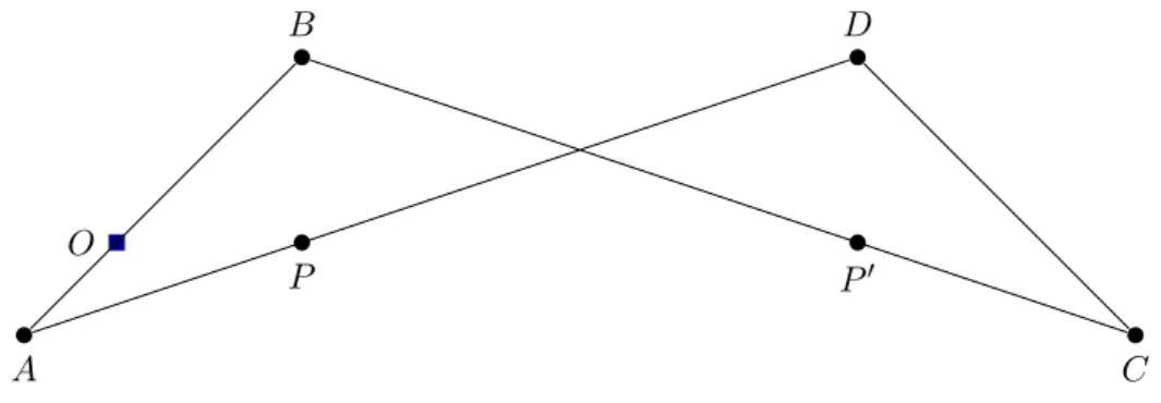
Figure 1.12 – Hart’s inversor. The bars AB and DC have the same length, as well as the bars AD and BC. The point O is located on the bar AB, so that AO/AB = µ. Likewise, P is on the bar AD, P� is on the bar CB, and AP/AD = CP�/CB = µ. It may be shown that P� is the image of P by inversion with respect to a circle of center O (for a proof, see [DO07] for example).

(23)

(24)

Part I

Universality theorems for linkages

in homogeneous surfaces

(25)

(26)

Chapter 2

Introduction and generalities on

universality

Throughout Part I, we shall consider linkages which are not necessarily planar: the ambiant space may be any manifold M instead of R2_.

A realization of a linkage _{L in a manifold M is a mapping which sends each vertex of} the graph to a point ofM, respecting the lengths of the edges. The conﬁguration space Conf_M(_{L) is the set of all realizations of L in M. This supposes, classically, the ambient} manifold_{M to have a Riemannian structure: thus the conﬁguration space may be seen} as the space of “isometric immersions” of the metric graphL in M.

Here we will always deal with (trivially) marked connected graphs, that is, a non-empty set of vertices have fixed realizations (in fact, when_{M is homogeneous, considering} a linkage without fixed vertices only adds a translation factor to the configuration space). Hence, our configurations spaces will be compact even if_{M is not compact, but rather} complete.

2.1 Some historical background

Most existing studies deal with the special case where M is the Euclidean plane and some with the higher dimensional Euclidean case (see for instance [Far08] and [Kin98]). There are also studies about polygonal linkages in the standard 2-sphere (see [KM+₉₉_]), or in the hyperbolic plane (see [KM96]).

Universality theorems. When M is the Euclidean plane E2_{, a conﬁguration space is an}

algebraic set. This set is smooth for a generic length structure on the underlying graph. Universality theorems tend to state that, playing with mechanisms, we get any algebraic set of Rn, and any manifold, as a conﬁguration space! In contrast, it is a hard task to understand the topology or geometry of the conﬁguration space of a given mechanism, even for a simple one.

Universality theorems have been announced in the ambient manifoldE2 by Thurston in oral lectures, and then proved by Kapovich and Millson in [KM02]. They have been proved in En by King [Kin98], and in RP2 and in the 2-sphere by Mn¨ev (see [Mn¨e88] and [KM02]). It is our aim in PartIto prove them in the cases of: the hyperbolic plane H2_{, the sphere} _S2 _{and the (Lorentz-)Minkowski plane}_{M. These are simply connected}

homogeneous pseudo-Riemannian surfaces (the list of such spaces includes in addition the 25

(27)

Euclidean and the de Sitter planes). Then it becomes natural to ask whether universality theorems hold in a more general class of manifolds, for instance on Riemannian surfaces without a homogeneity hypothesis.

In order to be more precise, it will be useful to introduce partial conﬁguration spaces: for W a subset of the vertices of_{L, one deﬁnes Conf}W_M(_{L) as the set of realizations of} the subgraph induced by W that extend to realizations of L. One has in particular a restriction map: Conf_M(_{L) → Conf}W_M(_L).

If W =_{{a} is a vertex of L, its partial conﬁguration space is its workspace, i.e. the} set of all its positions in M corresponding to realizations of L.

Euclidean planar linkages. Now regarding the algebraic side of universality, the history starts (and almost ends) in 1876 with the well-known Kempe’s theorem [Kem76]: Theorem 2.1. Any algebraic curve of the Euclidean plane E2, intersected with a Eu-clidean ball, is the workspace of some vertex of some mechanical linkage.

This theorem has the following natural generalization, which we will call the algebraic universality theorem, proved by Kapovich and Millson (see [KM02]):

Theorem 2.2. Let A be a compact semi-algebraic subset (see Definition 2.12) of (E2)n (identified with R2n). Then, A is a partial configuration space ConfW_E2(L) of some linkage _{L in E}2_{. When A is algebraic, one can choose} _{L such that the restriction map}

Conf_E2(L) → A = ConfW_E2(L) is a smooth ﬁnite trivial covering.

When Conf_E2(L) is not a smooth manifold, as usual, by a smooth map on it, we mean the restriction of a smooth map deﬁned on the ambient R2n_.

From Theorem 2.2, Kapovich and Millson easily derive the diﬀerential universality theorem on the Euclidean plane:

Theorem 2.3. Any compact connected smooth manifold is diﬀeomorphic to one connected component of the conﬁguration space of some linkage in the Euclidean planeE2_{. More}

precisely, there is a configuration space whose components are all diffeomorphic to the given differentiable manifold.

Jordan and Steiner also proved a weaker version of this theorem with more elementary techniques (see [JS99]).

How to go from the algebraic universality to the differentiable one? The differentiable universality theorems (Theorems2.3, 2.5and2.7) follow immediately from the algebraic ones (Theorems2.2,2.4and2.6) once we know which smooth manifolds are diffeomorphic to algebraic sets. In 1952, Nash [Nas52] proved that for any smooth connected compact manifold M , one may find an algebraic set which has one component diffeomorphic to M . In 1973, Tognoli [Tog73] proved that there is in fact an algebraic set which is diffeomorphic to M (a proof may be found in [AK92], or in [BCR98]).

In the non-compact case (in which we will be especially interested), Akbulut and King [AK81] proved that every smooth manifold which is obtained as the interior of a compact manifold (with boundary) is diﬀeomorphic to an algebraic set. Note that conversely, any (non-singular) algebraic set is diﬀeomorphic to the interior of a compact manifold with boundary.

(28)

2.2. RESULTS 27

2.2 Results

It is very natural to ask if these algebraic and diﬀerential universality theorems can be formulated and proved for conﬁguration spaces in a general target space _{M. Our} results suggest this could be true: indeed, we naturally generalize universality theorems to the cases ofM = M, H2 _and_S2_{, the Minkowski and hyperbolic planes and the sphere,}

respectively. Notice that for a general_{M, there is no notion of algebraic subset of M}n! We will however observe that there is a natural one in the cases we are considering here. In the general case, the question around Kempe’s theorem could be rather formulated as: “Characterize curves in _{M that are workspaces of some vertex of a linkage.”}

Minkowski planar linkages. These linkages are studied in Chapter 3. Classically, the structure of_{M needed to define realizations of a linkage is that of a Riemannian manifold.} Observe however that a distance, not necessarily of Riemannian type, onM would also suffice for this task. But our idea here is instead to relax positiveness of the metric. Instead of a Riemannian metric, we will assume_{M has a pseudo-Riemannian one. We} will actually restrict ourselves to the simple flat case where M is a linear space endowed with a non-degenerate quadratic form, and more specially to the 2-dimensional case, that is the Minkowski plane_{M. On the graph side, weights of edges are no longer assumed} to be positive numbers. This framework extension is mathematically natural, and may be related to the problem of the embedding of causal sets in physics, but the most important (as well as exciting) fact for us is that configuration spaces are (a priori) no longer compact, and we want to see what new spaces we get in this new setting.

The Lorentz-Minkowski plane M is R2 endowed with a non-degenerate indeﬁnite quadratic form. We denote the “space coordinate” by x and the “time coordinate” by t.

The configuration space Conf_M(L) is an algebraic subset (defined by polynomials of degree 2) of Mn = R2n (n is the number of vertices of _{L), and similarly a partial} configuration space ConfW_M(_{L) is semi-algebraic (see Definiton} 2.12). In contrast to the Euclidean case, these sets may be non-compact (even if L has some fixed vertices in M). We will prove:

Theorem 2.4. Let A be a semi-algebraic subset of Mn (identified withR2n). Then, A is a partial configuration space ConfW_M(_{L) of some linkage L in M. When A is algebraic,} one can choose L such that the restriction map ConfM(L) → A is a smooth finite trivial

covering.

Somehow, considering Minkowskian linkages is the exact way of realizing non-compact algebraic sets! In particular, Kempe’s theorem extends (globally, i.e. without taking the intersection with balls) to the Minkowski plane: any algebraic curve is the workspace of one vertex of some linkage.

Remark. If the restriction map is injective, then it is a bijective algebraic morphism from Conf_M(L) to A, but not necessarily an algebraic isomorphism. In fact, it is true for non-singular complex algebraic sets that bijective morphisms are isomorphisms, but this is no longer true in the real algebraic case (see for instance [Mum95], Chapter 3).

We also have a differential version of the universality theorem in the Minkowski plane (which follows directly from Theorem2.4, as explained at the end of Section 2.1): Theorem 2.5. For any differentiable manifold M with finite topology, i.e. diffeomorphic to the interior of a compact manifold with boundary, there is a linkage in the Minkowski

(29)

plane with a configuration space whose components are all diffeomorphic to M . More precisely, there is a partial configuration space ConfW_M(L) which is diffeomorphic to M and such that the restriction map Conf_M(L) → ConfW

M(L) is a smooth ﬁnite trivial

covering.

Hyperbolic planar linkages. In Chapter 4, we prove that both algebraic and differential universality theorems hold in the hyperbolic plane. The problem is that the notion of algebraic set has no intrinsic definition in the hyperbolic plane. However, it is possible to define an algebraic set in the Poincaré half-plane model

�� x y � ∈ R2     y > 0 � (and hence in H2) as an algebraic set of R2 which is contained in the half-plane. In fact, it turns out that the analogous definitions in the other usual models (the Poincaré disc model, the hyperboloid model, or the Beltrami-Klein model) are all equivalent. With this definition, we obtain the same results as in the Euclidean case:

Theorem 2.6. Let A be a compact semi-algebraic subset of (_H2₎n _{(identiﬁed with a}

subset of R2n using the Poincaré half-plane model). Then, A is a partial configuration space of some linkage _{L in H}2. When A is algebraic, one can choose _{L such that the} restriction map Conf_H2(L) → A is a smooth finite trivial covering.

Conversely, any partial conﬁguration space of any linkage with at least one ﬁxed vertex is a compact semi-algebraic subset of (_H2₎n_{, so this theorem characterizes the sets which}

are partial conﬁguration spaces (see Deﬁniton 2.12for the notion of “semi-algebraic”). In particular, Kempe’s theorem holds in the hyperbolic plane.

And here follows the diﬀerential version:

Theorem 2.7. For any compact differentiable manifold M , there is a linkage in the hyperbolic plane with a configuration space whose components are all diffeomorphic to M . More precisely, there is a partial configuration space ConfW_H2(L) which is diffeomorphic to M and such that the restriction map Conf_H2(L) → ConfW_H2(L) is a smooth finite trivial covering.

Spherical linkages. These linkages are the subject of Chapter 5. In 1988, Mnëv [Mnë88] proved that the algebraic and differential universality theorems hold true in the real projective plane_RP2_{endowed with its usual metric as a quotient of the standard 2-sphere.}

Even better, he showed that the number of copies in the differential universality for RP2 can be reduced to 1, i.e. any manifold is the configuration space of some linkage. As Kapovich and Millson pointed out [KM02], a direct consequence of Mnëv’s theorem is the differential universality theorem for the 2-sphere (but, this time, we get several copies of the desired manifold):

Theorem 2.8 (Mnëv-Kapovich-Millson). For any compact differentiable manifold M , there is a linkage in the sphere with a configuration space whose components are all diffeomorphic to M .

However, it seems impossible to use Mn¨ev’s techniques to prove the algebraic univer-sality for spherical linkages: for example, all the conﬁguration spaces of his linkages are symmetric with respect to the origin of_R3_{. In order to obtain any semi-algebraic set as}

(30)

2.2. RESULTS 29 a partial conﬁguration space, we need to start again from scratch and construct linkages speciﬁcally for the sphere.

Contrary to the Minkowski and hyperbolic cases, the generalization of the theorems to higher dimensional spheres is straightforward. Thus, we are able to prove the following: Theorem 2.9. Let d_{≥ 2 and let A be a compact semi-algebraic subset of (S}d₎n_(identiﬁed

with a subset of R(d+1)n). Then, A is a partial conﬁguration space of some linkage L in Sd_.

In particular, Kempe’s theorem holds in the sphere.

Conversely, any partial conﬁguration space of any linkage is a compact semi-algebraic subset of (Sd)n (see Section2.4), so this theorem characterizes the sets which are partial conﬁguration spaces.

Let us note that even when A is algebraic, our construction does not provide a linkage L such that the restriction map ConfSd(L) → A is a smooth ﬁnite trivial covering. We do not know whether such a linkage exists.

Some questions. Our results suggest naturally – among many questions – the following: 1. Besides the 2-dimensional case, are the results in the Minkowski plane true for any (ﬁnite-dimensional) linear space endowed with a non-degenerate quadratic form? And what about higher-dimensional hyperbolic spaces? It is likely that the adaptation of the 2-dimensional proof hides no surprise, like in the Euclidean case, but it would probably require tedious work to prove it.

2. In our deﬁnition of linkages in the Minkowski plane, we allow some edges to have imaginary lengths (they are “timelike”). Is it possible to require the graphs of Theorems 2.4 and 2.5 to be spacelike, i.e. require all their edges to have real lengths?

3. In all the universality theorems that we prove, we obtain a linkage whose configu-ration space is diffeomorphic to the sum of a finite number of copies of the given manifold M . Is it possible to choose this sum trivial, that is, with exactly one copy of M ? (This question is also open in the Euclidean plane.)

4. Is the diﬀerential universality theorem true on any Riemannian manifold?

Linkages on Riemannian manifolds. Let us give a partial answer to the last question using the following idea: just as the surface of the earth looks ﬂat to us, any Riemannian manifold will almost behave as the Euclidean space if one considers a linkage which is small enough. However, our linkage has to be robust to small perturbations of the lengths, which is not the case for many of the linkages described in PartI(consider for example the rigidiﬁed square linkage).

Theorem 2.10. Consider a linkage _{L in the Euclidean space E}n_{, with at least one}

ﬁxed vertex, such that for any small perturbation of the length vector l ∈ (R≥0)E, the

configuration space Conf_En(L) remains the same up to diffeomorphism. Then for any Riemannian manifold _{M, there exists a linkage L}_M in _{M whose configuration space is} diffeomorphic to Conf_En(L).

(31)

In particular, Theorem 2.10combined with the work of Jordan and Steiner [JS01] yields directly

Corollary 2.11. In any Riemannian surface M, the differentiable universality theorem is true for compact orientable surfaces. In other words, any compact orientable surface is diffeomorphic to the configuration space Conf_M(_{L) of some linkage L.}

This leads to the following

Question. Which manifolds can be obtained as the conﬁguration space of some linkage in Rn _{which is robust to small perturbations (in the sense of Theorem}_2.10_{) ?}

This question is probably very diﬃcult, but it is clear that there are restrictions on such manifolds: for example, they have to be orientable (because of Proposition1.3).

2.3 Ingredients of the proofs

There are essentially three technical as well as conceptual tools: functional linkages, combination of elementary linkages, and regular inputs. The main idea is always the same as in all the known proofs of Universality theorems (see the proofs of Thurston, Mn¨ev [Mn¨e88], King [Kin98] or Kapovich and Millson [KM02]): one combines elementary linkages to construct a “polynomial linkage”.

Functional linkages. One major ingredient in the proofs is the notion of functional linkages. Here we enrich the graph structure by marking two new vertex subsets P and Q playing the role of inputs and outputs, respectively. If the partial realization of Q is determined by the partial realization of P , by means of a function f : ConfP_M(_{L) → M}Q (called the input-output function), then we say that we have a functional linkage for f (for us,M will be the Minkowski plane M, the hyperbolic plane H2 _{or the sphere} _Sd_).

The Peaucellier linkage is a famous historical example: it is functional for an inversion with respect to a circle. With the notations of Figure 1.9, the input is D and the output is E.

Combination. Another major step in the proofs consists in proving the existence of functional linkages associated to any given polynomial f . This will be done by “combining” elementary functional linkages. We deﬁne combination so that combining two functional linkages for the functions f1 and f2 provides a functional linkage for f1◦ f2.

Elementary linkages. All the work then concentrates in proving the existence of linkages for suitable elementary functions (observe that even for elementary linkages one uses a combination of more elementary ones). As an example, we give the list of the elementary linkages needed to prove Theorem2.4 (in the Minkowski case):

1. The linkages for geometric operations:

(a) The robotic arm linkage (Section3.2.1): one of the most basic linkages, used everywhere in our proofs and in robotics in general.

(b) The rigidiﬁed square (Section 3.2.2): a way of getting rid of degenerate conﬁgurations of the square using a well-known construction.

(32)

2.3. INGREDIENTS OF THE PROOFS 31 (c) The Peaucellier inversor (Section3.2.3): this famous linkage of the 1860’s has a slightly diﬀerent behavior in the Minkowski plane but achieves basically the same goal.

(d) The partial t0-line linkage (Section3.2.4): it is obtained using a Peaucellier

linkage, but does not trace out the whole line.

(e) The t0-integer linkage (Section3.2.5): it is a linkage with a discrete

conﬁgura-tion space.

(f) The t0-line linkage (Section3.2.6): it draws the whole line, and is obtained by

combining the two previous linkages.

(g) The horizontal parallelizer (Section3.2.7): it forces two vertices to have the same ordinate, and it is obtained by combining several line linkages.

(h) The diagonal parallelizer (Section 3.2.8): its role is similar to the horizontal parallelizer but its construction is totally diﬀerent.

2. The linkages for algebraic operations, which realize computations on the t = 0 line: (a) The average function linkage (Section3.3.1): it computes the average of two

numbers, and is obtained by combining several of the previous linkages. (b) The adder (Section 3.3.2): it is functional for addition on the t = 0 line, and

is obtained from several average function linkages.

(c) The square function linkage (Section 3.3.3): it is functional for the square function and is obtained by combining the Peaucellier linkage (which is func-tional for inversion) with adders. This linkage is somewhat diﬃcult to obtain because we want the inputs to be able to move everywhere in the line, while the inversion is of course not deﬁned at x = 0.

(d) The multiplier (Section3.3.4): it is functional for multiplication and is obtained from square function linkages.

(e) The polynomial linkage (Section3.3.5): obtained by combining adders and multipliers, it is functional for a given polynomial function f . This linkage is used to prove the universality theorems: if the outputs are ﬁxed to 0, the inputs are allowed to move exactly in f−1(0).

Regular inputs. In our theorems, we need the restriction map Conf_M(_{L) → Conf}P_M(_L) to be a smooth finite trivial covering. In the differential universality Theorem, it ensures in particular that the whole configuration space consists in several copies of the given manifold M . The set of regular inputs RegP_M(_{L) is the set of all realizations of the inputs} which admit a neighborhood onto which the restriction map is a smooth finite covering. We have to be very careful, because even for quite simple linkages such as the robotic arm, the restriction map is not a smooth covering everywhere! There are mainly two possible reasons for the restriction map not to be a smooth covering:

1. One realization of the inputs may correspond to inﬁnitely many realizations of the whole linkage (for example, when the robotic arm in Section 3.2.1has two inputs ﬁxed at the same location, the workspace of the third vertex is a whole circle).

(33)

2. Even if it corresponds only to a ﬁnite number of realizations, these realizations may not depend smoothly on the inputs (for example, when the robotic arm in Section3.2.1is stretched).

New difficulties in each case. While the idea is always the same in all known proofs of universality theorems for linkages, i.e. combine elementary linkages to form a functional linkage for polynomials, each case has its own new difficulties due to different geometric properties, and the elementary linkages always require major changes to work correctly. Here follow examples of such differences with the Euclidean case:

The Minkowski case

1. The Minkowski planeM is not isotropic: its directions are not all equivalent. Indeed, these directions have a causal character in the sense that they may be spacelike, lightlike or timelike. For example, one needs diﬀerent linkages in order to draw spacelike, timelike and lightlike lines.

2. In the Euclidean plane, two circles C(x, r) and C(x�_{, r}�_{) intersect if and only if}

|r −r�_{| ≤ �x−x}�_{� ≤ r +r}�_{, but in the Minkowski plane, the condition of intersection}

is much more complicated to state (see Section3.1.2).

3. In the Euclidean plane, one only has to consider compact algebraic sets. Applying a homothety, one may assume such a set to be inside a small neighborhood of zero, which makes the proof easier. Here, the algebraic sets are no longer compact, so we have to work with mechanisms which are able to deal with the whole plane.

The hyperbolic case

1. The rigidiﬁed square linkage, used extensively in all known proofs in the ﬂat case, does not work anymore in its usual form, and does not have a simple analogue. 2. There is no natural notion of homothety: in particular, the pantograph does not

compute the middle of a hyperbolic segment, contrary to the ﬂat cases. 3. The notion of algebraic set is less natural than in the ﬂat case.

4. In every standard model of the hyperbolic plane (such as the Poincar´e half-plane), the expression of the distance between two points is much more complicated than in the ﬂat case.

The spherical case

1. Just as in the hyperbolic case, the curvature prevents the rigidiﬁed square linkage from working correctly.

(34)

2.4. ALGEBRAIC AND SEMI-ALGEBRAIC SETS 33 3. In the Euclidean or hyperbolic planes, we only need to prove algebraic universality for bounded algebraic sets, which means that our functional linkages do not need to work on the whole surface. In the sphere, all the distances are uniformly bounded (even the lengths of the edges of our linkages), so we need to take into account the whole sphere when constructing linkages.

4. The compactness of the sphere also makes it diﬃcult to construct linkages which deal with algebraic operations (addition, multiplication, division) since there is no proper embedding of R in the sphere.

2.4 Algebraic and semi-algebraic sets

In this section, we recall the standard deﬁnitions of algebraic and semi-algebraic sets. We adapt them to the Minkowski plane, the hyperbolic plane and the sphere in a natural way and state some of their properties.

Deﬁnition 2.12. An algebraic subset ofRn is a set A_{⊆ R}n such that there exist m_{∈ N} and f :_Rn_{→ R}m _{a polynomial such that A = f}−1_(0).

We deﬁne a semi-algebraic subset ofRn(see [BCR98]) as the projection of an algebraic set1. More precisely, it is a set B such that there exists N _{≥ n and an algebraic set A of} RN _{such that B = π(A), where π is the projection onto the ﬁrst coordinates}

π :RN =Rn_{× R}N−n_{→ R}n (x, y)�−→ x.

We deﬁne the (semi-)algebraic subsets of Mn _{by identifying}_Mn _{with (}_R2₎n₌_R2n_.

We also define the (semi-)algebraic subsets of (H2)n, using the Poincaré half-plane model (see Definition 4.1), as the (semi-)algebraic subsets of R2n which are contained in �� x y � ∈ R2    y > 0 �n .

Finally, a (semi-)algebraic subset of (Sd₎n _{(for d}_{≥ 2) is a semi-algebraic subset of}

Rd+1 _{which is contained in the unit sphere of} _Rd+1_.

Proposition 2.13. For any compact semi-algebraic subset B of Rn, there exists N ≥ n and a compact algebraic subset A ofRN such that B = π(A), where π is the projection onto the ﬁrst coordinates: RN _{→ R}n_.

Proof. First case. Assume for the moment that there exist polynomials f1, . . . , fm :

Rn_{→ R such that} B =_{{x ∈ R}n _{| ∀i ∈ {1, . . . , m} f}i(x)≥ 0} . Let h :Rn+m =Rn_{× R}m_{→ R}m   x,    y1 .. . ym       �−→    f1(x)− y12 .. . fm(x)− y2m   

1_{Our deﬁnition of semi-algebraic sets is not the standard one, but we know from the Tarski–Seidenberg}

(35)

and A = h−1(0). Then the projection of A onto the ﬁrst n coordinates is obviously B. Moreover, A is compact since it is the image of B by the continuous function

g : B → Rn+m=Rn× Rm x�−→   x,    � f1(x) .. . � fm(x)      .

General case. The finiteness theorem for semi-algebraic sets (see [BCR98], 2.7.2) states that any closed algebraic set can be described as the union of a finite number of sets B1, . . . , Bk which satisfy the assumption of the first case: apply the first case to each

of the Bi’s to end the proof.

We end this section with two analogous propositions for the hyperbolic plane and the sphere.

Proposition 2.14. For any compact semi-algebraic subset B of (_H2₎n_{, there exists N} _{≥ n}

and a compact algebraic subset A of (H2)N (with some N ≥ n) such that B = π(A), where π is the projection onto the ﬁrst coordinates: (H2)N _{→ (H}2)n.

Proof. Let A�be a compact algebraic set ofRN�(with some N� ≥ 2n) such that B = π(A�_),

where π is the projection onto the ﬁrst coordinates: _RN� _{→ R}2n_{. Then the projection of}

the compact algebraic set

A := �� x1 y1 � , . . . , � xn yn � , � xn+1 1 � , . . . , � xN�_−n 1 �� _   (x1, y1, . . . , xn, yn, xn+1, . . . , xN�_−n)∈ A� � (where A⊆ (H2₎N�_−n ) is exactly B.

Proposition 2.15. For any compact semi-algebraic subset B of (S2)n, there exists N _{≥ n} and a (compact) algebraic subset A of (_S2₎N _{(with some N} _{≥ n) such that B = π(A),}

where π is the projection onto the ﬁrst coordinates: (S2)N → (S2₎n_.

Proof. Let A�be a compact algebraic set of_RN�_{(with some N}� _{≥ 3n) such that B = π(A}�_),

where π is the projection onto the ﬁrst coordinates: RN� _{→ R}3n. Since A� is compact, there is a λ such that π2(A�) ∈ [−λ, λ]N�−3n, where π2 is the projection onto the last

coordinates: RN� → RN�_−3n

. Then the projection of the compact algebraic set A :=         xy11 z1   , . . . ,  xynn zn   ,  xyn+1n+1 0   , . . . ,   x_{N �−2n} yN �−2n 0            � x1, y1, z1, . . . , xn, yn, zn, λxn+1, . . . , λx_{N �−2n} � ∈ A� x2n+1+ y2n+1= 1, . . . , x2N �−2n+ y 2 N �−2n= 1      (where A_{⊆ (S}2₎N�−2n_{) is exactly B.}

Of course, Proposition 2.15 extends toSdwith any d≥ 2.

2.5 Generalities on linkages

In the present section, we develop generalities on linkages which apply to the Minkowski plane, the hyperbolic plane and the sphere. Thus, we consider a smooth manifold_M endowed with a distance function