HAL Id: hal-00744131
https://hal.archives-ouvertes.fr/hal-00744131v2
Submitted on 30 May 2017
HAL is a multi-disciplinary open access
archive for the deposit and dissemination of
sci-entific research documents, whether they are
pub-lished or not. The documents may come from
teaching and research institutions in France or
abroad, or from public or private research centers.
L’archive ouverte pluridisciplinaire HAL, est
destinée au dépôt et à la diffusion de documents
scientifiques de niveau recherche, publiés ou non,
émanant des établissements d’enseignement et de
recherche français ou étrangers, des laboratoires
publics ou privés.
Alain Ajami, Jean-Paul Gauthier, Thibault Maillot, Ulysse Serres
To cite this version:
Alain Ajami, Jean-Paul Gauthier, Thibault Maillot, Ulysse Serres. How humans fly. ESAIM:
Con-trol, Optimisation and Calculus of Variations, EDP Sciences, 2013, 19 (4),
https://www.esaim-cocv.org/articles/cocv/abs/2013/04/cocv120043/cocv120043.html.
�10.1051/cocv/2012043�.
�hal-00744131v2�
DOI:10.1051/cocv/2012043 www.esaim-cocv.org
HOW HUMANS FLY
Alain Ajami
1, Jean-Paul Gauthier
1,2, Thibault Maillot
1and Ulysse Serres
3,4 Abstract.This paper is devoted to the general problem of reconstructing the cost from the observation of trajectories, in a problem of optimal control. It is motivated by the following applied problem, concerning HALE drones: one would like them to decide by themselves for their trajectories, and to behave at least as a good human pilot. This applied question is very similar to the problem of determining what is minimized in human locomotion. These starting points are the reasons for the particular classes of control systems and of costs under consideration. To summarize, our conclusion is that in general, inside these classes, three experiments visiting the same values of the control are needed to reconstruct the cost, and two experiments are in general not enough. The method is constructive.The proof of these results is mostly based upon the Thom’s transversality theory.
This study is partly supported by FUI AAP9 project SHARE, and by ANR Project GCM, program “blanche”, project number NT09-504490.
Mathematics Subject Classification. 93C10, 49J15, 93C41, 93C15, 34K35.
Received May 14, 2012. Revised October 16, 2012. Published online June 3, 2013.
1. Introduction
This study holds in the context of the french FUI SHARE project (see [2]), and authors are granted from the project.
From the kinematic point of view, a rough HALE drone (high altitude, long endurance drone) is governed by the standard Dubins equations: ⎧
⎪ ⎨ ⎪ ⎩ ˙x = cos θ ˙y = sin θ ˙θ = u. (1.1)
These equations express that the drone moves on a perfect plane (perfect constant altitude), at perfect constant speed 1, moves in the direction of its velocity vector, and is able to turn right and left.
Keywords and phrases. Inverse optimal control, anthropomorphic control, transversality.
1 Université du Sud-Toulon-Var, LSIS, UMR CNRS 7296, B.P 20132, 83957 La Garde Cedex, France. [email protected]; [email protected]; [email protected]
2 INRIA GECO Project
3 Université de Lyon, 69 622 Lyon, France
4 Université Lyon 1, Villeurbanne; LAGEP, UMR CNRS 5007, 43 bd du 11 novembre 1918, 69100 Villeurbanne, France. [email protected]
These equations were also considered by people studying human locomotion: see the seminal works of Chitour-Jean-Mason [8], and Chittaro-Jean-Mason [10]. See also older but basic works of Laumond [3–5], who originally introduced this point of view.
Another typical result related with cost reconstruction in human movements is [6,7,11]. A part of the methodology in [6,7,11] is very similar to what we do here in.
Note that the rough model (1.1) is more pertinent as a model of the kinematics of HALE drones than as a model of human locomotion: actually, for HALE drones, the velocity is almost really constant5.
Once this assumption of constant velocity is accepted, the natural requirement of invariance under motions of the plane leads to these equations.
In both cases but for different reasons, the assumption is that some integral cost is minimized, to connect in free time, the initial and target point. Again, the natural requirement of invariance with respect to motions of the plane leads to an integral cost of the form:
C(u(·)) = % T
0
L(u(t), ˙u(t), . . . , u(k)(t))dt (1.2) In the case of human locomotion, a very interesting argument of dimension of a certain set shows that k = 1 in equation (1.2) above (see [13]). We discuss this in more details in Sections 3.3, 5. Shortly, the results here provide a clear method to validate this assumption k = 1.
It turns out, and this is quickly shown in Section 5, that the measurement of two different trajectories is enough to reconstruct the cost L(u) (over the set of values of u(t) visited during the two experiments), provided that both experiments visit the same value of the control (at different times, maybe).
These considerations are the starting point of this study, and the reason to consider the following class of nonlinear control affine systems, with single control u, and of costs C(u(·)):
& ˙x = f(x, y)
˙y = u (1.3)
where x is n-dimensional, and the cost
C(u(·)) = % T
0
L(u(t))dt. (1.4)
Surprisingly, our main result is the following rough statement, the precise result being Theorem 4.1, Section4.1.
Theorem 1.1 (rough statement). To reconstruct the cost (1.4), three experiments are in general enough pro-vided that they visit the same value of the control, at some (maybe different) instants. Two experiments are in general not enough.
Hence, in fact, the Dubins case is, inside its class, very particular. This is due to the symmetries (invariance of the problem under the action of motions of the plane).
Moreover, in both cases (Dubins case and case (1.3)), the reconstruction of L can be made only up to a linear term, which is in fact totally irrelevant: adding a linear term to L does not change the set of optimal trajectories. On the contrary, for completely general affine control systems, this additional degree of freedom does not (generically) exist.
In the paper, we finish by considering (more quickly) the case of a general control affine system, ˙q = F0(q) +
uF1(q) (Sect. 6). It turns out that the main Theorem1.1still holds. Even a bit more: now L(u) is completely
determined by three experiments (not up to some linear term).
The organization of the paper is as follows:
- In Sections 2, 3, we give a clear statement of the problem, together with all prerequisites necessary to the mathematical precise understanding of the paper. A key lemma for the proofs (Lem.3.17) is established. The very short Section3.3concerns our conclusion about the validation of the assumption that the cost C(u(·)) is of the form (1.4).
- Section 4 is devoted to the results of our study. In Section4.1 we give a clear statement of our main result and in Section 4.2 we give the crucial preliminaries for the proof of the main result (Thm. 4.1). Section
4.3.2regroups, besides the final proof, all technical lemmas, and the proof of the fact that in general two experiments are not enough.
- Section5deals with Dubins case, and the application to HALE drones. - Section6cares about the case of general control affine systems (very shortly).
2. Statement of the problem
In this paper, smooth means C∞. Also, we do not distinguish between row and column vectors, the distinction
being clear from the context.
2.1. Systems under consideration
As we said in the introduction, we deal with single input nonlinear control affine systems of the form (1.3), with (x, y) ∈ X × Y , the state variable and u ∈ R, the control variable. Here, X (resp. Y ) is an n-dimensional (resp. one-dimensional) connected, Hausdorff and paracompact smooth manifold.
Setting q = (x, y) and Q = X × Y , we rewrite the system (1.3) as
˙q = F0(q) + uF1(q), q∈ Q, u ∈ R, (2.1)
where F0 = (f, 0) and F1 = (0, 1) are smooth vector fields on Q. Depending on the context, we will use freely
the most convenient notation between both.
Let F denote the set of smooth control systems form (1.3) or (2.1), i.e., elements of F are smooth vector fields F0 on Q such that F0 : Q → T X × {0T Y}. Equivalently, elements of F are y-parametrized families of
smooth vector fields f over X, i.e., smooth sections of a vector bundle over Q with fiber TxX. Let JkF denote
the bundle of k-jets of systems in F.
The set of admissible control functions u(·) is as usual L∞
loc(R+,R), and the set of admissible trajectories is
the set of solutions of system (1.3) or (2.1) corresponding to an admissible control function u(·). The domain of our control functions will be a certain time interval [t1, t2] depending on u(·). If necessary, it is always possible
to assume that t1= 0.
2.2. Problem under consideration
2.2.1. Main assumption
Our main assumption in the paper is: all trajectories occuring in the observations are solutions of an optimal control problem of the following form, that we shall denote by (PL).
(PL) Minimize the integral cost (1.4) among all admissible controls u(·) steering system (2.1) from a source point
q0 to a target point q1 in free final time T .
We do not consider arbitrary functions L in the functionals C(u(·)) above: indeed, we choose a class L ensuring that the optimal control problem (PL) has a solution for each L in L. Following [8,10], L is the set of
L :R → R meeting the following assumptions: (A1) L(·) is strictly positive and smooth;
(A2) L(·) is strictly convex with L′′(u) > 0 (i.e., strictly strongly convex);
2.2.2. The different notions of experiments
Among the set of admissible pairs (q(·), u(·)), we shall distinguish the ones called experiments:
Definition 2.1 (experiment). An admissible trajectory (q(·), u(·)) is called an experiment if there exists L ∈ L such that (q(·), u(·)) solves (PL).
Remark 2.2. Since a solution of system (2.1) is uniquely determined by the initial condition q0 in Q and the
admissible control function u(·), we may identify an experiment (q(·), u(·)) with a pair (q0, u(·)). For simplicity,
we shall denote indifferently both by γ.
We also denote by Γf a family of experiments whose corresponding trajectories q(·) are solutions to
system (2.1).
Definition 2.3 (compatible experiments). A family Γfof admissible pairs γ = (q, u(·)) is a family of compatible
experiments if there exists (a common) L ∈ L such that every γ ∈ Γf, solves (PL).
Definition 2.4 (monotonic experiment). An experiment (q(·), u(·)) is monotonic if the control function u(·) is smooth monotonic (strictly, i.e., u′(t) does not vanish for any t).
From now on we consider monotonic experiments only. In particular, the mapping u %→ t(u) is well defined, continuous and smooth, i.e., belongs to U = C∞(R
+,R). The smoothness assumption, that may look not very
reasonable, will be justified later (Lem.3.5).
In the following, with a little abuse of notations, a time dependent function g is written g(u) instead of g(t(u)) whenever necessary. Also, we use the dot ˙ to denote the derivative with respect to time t, and the prime′ to
denote the derivative with respect to variable u.
Definition 2.5 (different experiments). Several experiments (qi(·), ui(·)), i = 1, . . . , ℓ, that visit common
con-trol values (i.e., such that the ranges of the associated concon-trol functions ui(·) overlap) are said to be different
if there are points t such that qi(t) ̸= qj(t) for all i ̸= j, on the overlapping range of control values.
Remark 2.6. A few obvious but useful observations are in order:
(i) The control of a monotonic experiment can take the value zero at most once. (ii) Let Γf be a family of experiments that visit common control values, namely,
∃ u0∈ R ∀ γ = (q0, u(·)) ∈ Γf ∃ t(γ) ∈ R+ | u(t(γ)) = u0,
we may assume without loss of generality that t(γ) = 0 for each experiment (shift of time on the experiments).
2.2.3. Statement of the inverse optimal control problem
The inverse optimal control problem that we shall denote by ( PL ) is the following.
( PL ) Given a family Γf of experiments, find a cost L in L such that every γ ∈ Γf solves (PL).
3. Study of the optimal control problem and its inverse
3.1. Study of the optimal control problem (P
L)
3.1.1. Existence of optimal controlsWe follow exactly the same lines as in [10, Sect. 3.1] for questions dealing with the existence of optimal controls. The growth condition L(u)! c|u|p with c > 0 and p > 1 used in [10, Sect. 2.1], has been weakened to
A3 according to [18, Thm. 2.8.1], and thus we can state the following.
Theorem 3.1. For every q0, q1∈ Q such that q1 is reachable from q0, there exists a real positive time T∗ and
a control function u(·) ∈ L1([0, T∗]) such that the corresponding trajectory q(·) solves problem (P L).
Notice that Theorem 3.1 does not provide the boundedness of the optimal controls. It will follow from Lemma 3.5.
Remark 3.2. Observe that the existence of a bounded positive T∗ is not completely trivial and follows from
the special form of the cost function L. Indeed, it follows easily from assumptions A1 and A3 that there exists a positive real number α such that L(u) > α for every u. Now, if q1is attainable from q0, let un(·) : [0, Tn] → Q
be a minimizing sequence. Then,
αTn< C(un(·)) < +∞,
which implies that Tn must be uniformly bounded.
3.1.2. Application of the Pontryagin Maximum Principle
Since we do not know yet that optimal controls are bounded in the L∞topology, we cannot apply the PMP
in its classical version. Nonetheless, it is easy to check that problem (PL) meets all the hypotheses required
in [18, Thm. 8.7.1] (a more refined version of PMP valid for unbounded controls), and thus we can state the following.
Proposition 3.3. Every solution to (PL) satisfies the PMP.
In order to apply the PMP to the problem (PL), we define the following Hamiltonian function:
h(λ, p, q, u) = ξf (q) + ζu + λL(u), with p = (ξ, ζ) ∈ T∗
qQand λ" 0.
An extremal curve is by definition a quadruple (λ, p(·), q(·), u(·)), meeting the following necessary conditions for optimality.
We recall that the PMP states that if q(·) is an optimal trajectory corresponding to a control u(·) defined on an interval [0, T ], then there exist an absolutely continuous curve p(·) : [0, T ] → T∗
q(·)Qand λ" 0 such that the
pair (λ, p(t)) never vanishes and for a.a. t ∈ [0, T ], (q(·), p(·)) satisfies the Hamiltonian system: ⎧ ⎪ ⎪ ⎨ ⎪ ⎪ ⎩ ˙q(t) = ∂h ∂p(λ, p(t), q(t), u(t)) ˙p(t) = −∂h ∂q(λ, p(t), q(t), u(t)), (3.1) and the maximality condition:
h(λ, p(t), q(t), u(t)) = max
v∈R h(λ, p(t), q(t), v). (3.2)
Also, since the final time is free, the Hamiltonian is identically zero along the optimal trajectory, namely, ξ(t)f (q(t)) + λL(u(t)) + ζ(t)u(t) = 0. (3.3) If λ ̸= 0, the extremal is called normal, while if λ = 0, the extremal is called abnormal. Notice that abnor-mal extreabnor-mals are extreabnor-mal (and often optiabnor-mal) for any cost since in this case the cost disappears from the Hamiltonian.
Remark 3.4. Here we have to face problems, due to the fact that abnormal trajectories come unavoidably in the picture:
- abnormal extremals, if they are not normal at the same time, cannot provide any information on the system. Hence we have to exclude them from our study;
- abnormals that are normal at the same time are automatically smooth (Lem.3.5below). Hence we can assume smoothness of our experiments.
- In fact, and for a purely technical reason, certain trajectories that are not abnormal cause problems: those that are abnormal on a piece of themselves only. We shall also exclude them, however, this exclusion can certainly be avoided.
3.1.3. Description of normal extremals of (PL)
In this case, since λ ̸= 0 we can normalize and assume that λ = −1. In this case, the maximality condition (3.2) rewrites
h(λ, p(t), q(t), u(t)) = max
v∈Rh(−1, p(t), q(t), v) = ξ(t)f(q(t)) + L ∗(ζ(t)),
with L∗(ζ) = maxu(ζu − L(u)) being the Legendre transform of L. The properties of the Legendre transform
imply the following relations between the optimal control u(·) and ζ(·):
u(t) = L∗′(ζ(t)), ζ(t) = L′(u(t)), (3.4) so that the maximality condition (3.3) may be rewritten as
L(u(t))− u(t)L′(u(t)) = ξ(t)f(q(t)). (3.5) The equation for q in (3.1) is nothing but (1.3), while the equation for p, also called the adjoint equation, can be explicitly rewritten using ξ and ζ. Summing up, all the information is contained in the system below:
⎧ ⎪ ⎪ ⎪ ⎪ ⎪ ⎪ ⎪ ⎪ ⎪ ⎨ ⎪ ⎪ ⎪ ⎪ ⎪ ⎪ ⎪ ⎪ ⎪ ⎩ ˙x = f(x, y) ˙y = u = L∗′(ζ) ˙ξ = −ξ∂f ∂x(x, y) ˙ζ = −ξ∂f ∂y(x, y) L∗(ζ) + ξf(x, y) = 0. (3.6)
3.1.4. Smoothness of (normal) optimal controls
Lemma 3.5. The optimal controls u(t) corresponding to normal trajectories of (PL) are smooth.
Proof. Assumption A2 implies that L∗′is a smooth function. Hence, u is smooth as a component of the solution
of a smooth differential system. #
Remark 3.6. Here is a place where the strong strict convexity is important. This assumption also implies that the set of costs under consideration is an open set. Also, it will be crucial in the normalizations of our costs later, and at the end in the possibility to determine uniquely the initial covectors associated with our experiments.
A by-product of Lemma 3.5is that in fact our extremal controls are also extremals of the standard (L∞ loc)
PMP (see [1,15]).
3.1.5. Characterization of abnormal extremals of (PL)
As we have already said, certain abnormal extremals will come in the picture. Then we shall characterize them.
First, let us introduce the resolvent R(t, t0) of the time-varying linear system (3.6) (third equation) to be the
matrix solution to ˙R = −R∂f
∂x, R(t0, t0) = IdRn (when t0= 0 we shall write R(t) instead of R(t, 0)), and define
the mapping V through the following lemma.
Lemma 3.7. To every monotonic smooth trajectory (q0, u(·)), q0 = (x0, y0), we can associate a well-defined
smooth map V (·) : U → Tx0X, defined over the range U of t %→ u(t), such that for every covector ξ0 in Rn and
every u that belongs to the value set of the control, we have
Proof. Since the covector ξ(t) satisfies the linear differential equation ˙ξ = −ξ∂f
∂x, ξ(t) = ξ0R(t, t0).
Ob-viously, the matrix R depends only on the experiment so that we can write (ξf)(t(u)) = ξ0V (u), with
V (u) = R(t(u), t0)f(q(t(u)). #
Lemma 3.8. The (monotonic smooth) trajectory t %→ q(t) = (x(t), y(t)), is the projection of an abnormal extremal if and only if span {V (u), u ∈ U} ̸= Tx0X ≃ Rn (or, equivalently, if and only if span {V (u(t)), t ∈
[0, T ]} ̸= Rn).
Proof. Assume first that q(·) is the projection of an abnormal extremal. Therefore, and since λ = 0, there exists a non trivial covector p(·) = (ξ(·), ζ(·)) such that
h(0, p(t), q(t), u(t)) = ξ(t)f (q(t)) + ζ(t)u(t) = max
v∈Rh(0, p(t), q(t), v).
The maximum being reached in the above equation, we necessarily have ζ(t) = 0 for all t ∈ [0, T ], and then, ξ(t)̸= 0 for every t ∈ [0, T ]. Consequently, the zero-hamiltonian condition reads ξ(t)f(q(t)) = 0, for all t ∈ [0, T ] or equivalently, for all u ∈ U,
ξ(0)V (u) = 0, (3.8)
with ξ(0) ̸= 0. This last equation (3.8) exactly means that {V′(u), u ∈ U} does not span T x0X.
Conversely, assume that {V (u), u ∈ U} does not span Tx0X. Thus, there exists ξ0∈ Tx∗0X such that ξ0V (u) =
0 for every u ∈ U, or, equivalently, that for all t ∈ [0, T ],
ξ(t)f (q(t)) = 0, (3.9)
with ξ(·) being the solution to the Cauchy problem ˙ξ = −ξ∂f
∂x(q(t)), ξ(0) = ξ0. Differentiating this last
equa-tion (3.9) with respect to t leads to
0 = ˙ξ(t)f(q(t)) + ξ(t)'∂f ∂x(q(t)) ˙x + ∂f ∂y(q(t)) ˙y ( = ξ(t)∂f ∂y(q(t)) ˙y = − ˙ζ(t)u(t),
which implies that ˙ζ(·) vanishes identically (by strict monotonicity, the control function u(·) vanishes at most once on [0, T ]). Hence, the optimal trajectory t %→ q(t) is the projection onto X ×Y of the abnormal extremal t %→
(0, ξ(t), 0, q(t), u(t)). This ends the proof. #
Lemma 3.9. Let γ : I → RN be a smooth curve, defined on some nontrivial interval I. Then, the two following
assertions are equivalent.
1. For any subinterval J ⊂ I, span {γ(t), t ∈ J} = RN,
2. The set of t0 such that span {γ(t0), γ′(t0), . . . , γ(N−1)(t0)} = RN is (open) dense in I.
Proof. The direct implication: we prove the result by contraposition. Assume that on some open subinterval ˜
I⊂ I, span {γ(t), . . . , γ(N−1)(t)} ̸= RN. For every integer i, define
r(i) = sup
t∈ ˜I
rank {γ(t), . . . , γ(i)(t)},
and let k be the first integer for which r(k) ̸= k + 1, namely r(k) = k. Let J ⊂ ˜I be a subinterval on which span{γ(t), . . . , γ(k−1)(t)} = Rk. For every t ∈ J, there exist α
0(t), α1(t), . . . , αk−1(t) such that γ(k)(t) = k−1 ) i=0 αi(t)γ(i)(t). (3.10)
Notice that the coefficients αi(·)’s are smooth on J. Indeed, relation (3.10) may be rewritten in matrix form as γ(k)(t) =*γ(t), . . . , γ(k−1)(t)+ ⎛ ⎜ ⎝ α0(t) ... αk−1(t) ⎞ ⎟ ⎠ ,
which can be smoothly solved in the αi(t)’s (i = 1, . . . , k − 1) since rank{γ(t), . . . , γ(k−1)(t) | t ∈ J} = k. Let
t0 ∈ J and let ˜R(t, t0) be the resolvent of the linear differential equation (3.10), i.e., ˜R(t, t0) is the matrix
solution to the Cauchy problem d
dtR(t, t˜ 0) = A(t) ˜R(t, t0), ˜R(t0, t0) = IdRk, with A(t) = ⎛ ⎜ ⎜ ⎜ ⎜ ⎝ 0 1 0 · · · 0 ... ... ... ... ... 0 . . . 0 1 0 0 . . . 0 1 α0 . . . αk−1 ⎞ ⎟ ⎟ ⎟ ⎟ ⎠. We have * γ(t), γ(k−1)(t)+=*γ(t0), γ′(t0), . . . , γ(k−1)(t0) + ˜ R(t, t0)∗,
with ˜R(t, t0)∗ being the transpose of ˜R(t, t0). Consequently, for all t ∈ J,
γ(t) = k ) i=1 ˜ Ri 1(t, t0)γ(i−1)(t0), with ˜Ri
1(t, t0) being the i-th element of the first line of matrix ˜R(t, t0). Therefore, γ(J) ⊂ Rk−1 and
conse-quently γ(·) does not span RN in restriction to J.
We now prove the converse. If γ does not span RN in restriction to some nontrivial interval J, there exists
k < N and a k-dimensional subspace Ek
⊂ RN such that γ(J) ⊂ Ek. Consequently, for every t ∈ J and every
integer i, we have γ(i)(t) ∈ Ek. This completes the proof. #
Definition 3.10 (normal experiment). A monotonic experiment (q(·), u(·)), defined on some time interval [0, T ] is normal if q(·) is not the projection of an extremal which is abnormal on [0, T ].
Definition 3.11 (normal-regular experiment). A monotonic experiment (q(·), u(·)), defined on some time in-terval [0, T ] is normal-regular if q(·) is not the projection of an extremal which is abnormal on some (nontrivial) subinterval of [0, T ].
Remark 3.12. Note that a normal experiment maybe non normal-regular.
By Lemma3.8, the experiment is normal-regular if V (u) (resp. V (t)) spans Rnin restriction to any nontrivial
subinterval of [u0, uT] (resp. [0, T ]).
As we said, we want to avoid trajectories such that a piece of them is abnormal, (i.e., non normal-regular experiments). An immediate consequence of Lemma3.9is the following corollary (one has to apply Lem.3.9to the curve u %→ V (u)).
Corollary 3.13. The (monotonic) trajectory, t %→ q(t) is normal-regular if and only if the set of u such that span{V (u), . . . , V(n−1)(u)} = Rn is (open) dense in [u
3.1.6. Test of abnormality
A reasonable practical test of abnormality is the standard Gram-matrix test. It may be done either using V (t) or V (u). We will write V (τ) to emphasize the fact that both can be indifferently considered. Define the Gram matrix relative to the interval [τ1, τ2] as:
Ga=
% τ2
τ1
V (τ )V∗(τ)dτ, where V∗ denotes the transpose of V .
It is clear that span{V (τ), τ ∈ J} = RN iff the symmetric matrix G
a is positive definite, iff its smallest
eigenvalue is strictly positive. Then, the test resumes to decide whether a matrix is positive definite which is standard in practice (see e.g. [16] and Ref. [6] therein).
Differentiating ξ0V (t) as was already done above, we get 0 = ξ0V′(t) = ξ0R(t)∂f∂y(q(t)). This leads to the
standard fact that linearization is not controllable along abnormals.
3.2. Study of the inverse optimal control problem
3.2.1. Well-posedness of the inverse control problem
The next lemma will show that the inverse control problem ( PL ) is an ill-posed problem.
Lemma 3.14. Assume that L ∈ L. Let a, b be arbitrary real numbers with a > 0. Set ˜L(u) = aL(u) + bu. An experiment relative to L is also an experiment relative to ˜L.
Proof. For abnormal experiments the result is obvious.
Let (q(·), u(·)) be a (normal) experiment relative to L. Then, there exists a covector p(·) = (ξ(·), ζ(·)) such that the extremal (−1, p(·), q(·), u(·)) is solution to system (3.6).
Consequently, since L∗(ζ) = sup
u(ζu − L) =1asupu((aζ + b)u − ˜L) = 1aL˜∗(aζ + b), one easily infers that the
extremal (−1, ˜p(·), q(·), u(·)), with ˜p = (˜ξ, ˜ζ) = (aξ, aζ + b), satisfies ⎧ ⎪ ⎪ ⎪ ⎪ ⎪ ⎪ ⎪ ⎪ ⎪ ⎪ ⎨ ⎪ ⎪ ⎪ ⎪ ⎪ ⎪ ⎪ ⎪ ⎪ ⎪ ⎩ ˙x = f(x, y) ˙y = u = ˜L∗′(˜ζ) ˙˜ξ= −˜ξ∂f∂x(x, y) ˙˜ζ = −˜ξ∂f∂y(x, y) ˜ L∗(˜ζ) + ˜ξf(x, y) = 0,
showing that (q(·), u(·)) is an experiment relative to ˜L. # 3.2.2. Normalization of the cost function
Lemma3.14shows that the projections onto the base manifold of the extremal trajectories of problems (PL)
and (PaL+bu) are the same. In particular it says that the cost reconstruction is an ill-posed problem.
One can only expect to reconstruct a class representative of the cost function under the equivalence relation ∼, ˜
L∼ L if there exists a real a > 0 and a real b such that ˜L(u) = aL(u) + bu. It is worth mentioning that under this equivalence relation the minimum of the cost function is not preserved but the set of control values such that L(u) − uL′(u) = 0 is preserved (indeed, due to assumption A1, A2, A3, there exist exactly two values for
which this relation holds: draw the tangents to the graph of L through the origin).
The following lemma gives a way to select a special class representative for the cost function.
Lemma 3.15 (resetting lemma). At u0 the cost function L to be reconstructed can be normalized so
that: L′(u
Proof. Let L be a class representative of the cost we aim to reconstruct. In order to get the required normal-ization, we need to solve for a, b real numbers, with a > 0 the following system
' L′(u 0) 1 L′′(u0) 0 ( ' a b ( = ' 0 1 ( ,
which is always possible for a cost function L in L: the coefficient a obtained in this way is positive (a = 1/L′′(u 0))
due to the strong convexity hypothesis. #
Remark 3.16. Notice that our normalization does not preserve the set L: after normalization, the assump-tion A1 may not hold, but this will be of no importance in the following. In fact the right way to define the class L would be to replace the positiveness of L by the weaker L(0) > 0. But this is unnatural for the purpose of proving the existence of minimizers (Thm.3.1).
3.2.3. Existence and uniqueness of the reconstructed cost
Lemma 3.17. Fix a system f in F and a smooth admissible trajectory (q(·), u(·)), with u(·) monotonic and defined on some time interval [t1, t2]. Fix a covector ξ0∈ Rn\{0}. Then, there exists a unique smooth function L
defined over the range of t %→ u(t), and such that L′(u(t
0)) = 0 for some arbitrary point t0∈ [t1, t2], for which the
pair (q(·), u(·)) is the projection of a normal extremal of problem (PL) associated with the covector (ξ(·), ζ(·)),
(ξ(t0), ζ(t0)) = (ξ0, 0).
Proof. Choose t0∈ [t1, t2] and set u0= u(t0), q0= q(t0). Let V (·) be the function associated to (q(·), u(·)) and
defined over the range of u(·) accordingly to Lemma3.7.
We begin with the existence of L and we also give a formula for it. The range of u is [u1, u2]. Assume u0̸= 0.
Consider any a ∈ [u1, u2]. The reader can easily check that
L(u) = ξ0V (u0) + (ξ0V (u0) − ξ0V (a)) ' u u0− 1 ( + u% u u0 ξ0V (a)− ξ0V (v) v2 dv, (3.11) is such that L′(u 0) = 0, and satisfies L(u)− uL′(u) = ξ 0V (u). (3.12)
If 0 /∈ [u1, u2], this L(u) is smooth and is the unique solution of the standard ODE (3.12) with L(u0) =
ξ0V (u0), L′(u0) = 0. If 0 ∈ [u1, u2], let us chose a = 0. Define the function g by g(u) = ξ0V (0)− ξ0V (u). We
have
g′(u) = −ut′(u)ξ(t(u))∂f
∂y(q(t(u))).
Hence, g(0) = g′(0) = 0, and we may write, g(u) = u2˜g(u), with ˜g smooth. L(u) = ξ
0V (u0) + (ξ0V (u0) −
ξ0V (0)(uu0 − 1) + u2uu0˜g(v)dv is a smooth solution of (3.12), with again L(u0) = ξ0V (u0), L′(u0) = 0.
Suppose now that u0= 0. Then, set L(u) = ξ0V (u0) + u2 u 0
ξ0V (0)−ξ0V (v)
v2 dv. Again, L(u) − uL′(u) = ξ0V (u),
g(u) = u2˜g(u), with ˜g smooth. L(u) = ξ
0V (u0) + u2 u
0 ˜g(v)dv, is a smooth function that meets L(0) = ξ0V (u0),
L′(0) = 0.
Note that the solution L(u) is well defined and smooth over the full interval [u1, u2].
We now prove uniqueness, when 0 ∈ [u1, u2]. We assume that 0 ∈ [u0, u2] (the case 0 ∈ [u1, u0] is similar).
Let L1 and L2 be two solutions to equation (3.12) such that L′1(u0) = L′2(u0) = 0. Then, ψ = L1− L2 is
a C∞ solution to
ψ(u)− uψ′(u) = 0, ψ(u0) = 0, ψ′(u0) = 0.
If u0is nonzero, then ψ (a smooth function) is identically zero on [u0, 0]. On ]0, u2], we must have ψ(u) = Ku,
It remains to prove that the pair (q(·), u(·)) is the projection of an extremal trajectory of the problem (PL).
By hypothesis, the given trajectory is an admissible trajectory of system (1.3).
By definition, V (u(t)) = R(t, t0)f(q(t)). Set ξ(t) = ξ0R(t, t0) so that ξ(·) satisfies the third equation of
system (3.6).
Set ζ(t) = L′(u(t)). Thus, ζ(t
0) = 0, and ˙ζ(t) = L′′(u(t)) ˙u(t) = −ξ0 V′(u) u ˙u(t) = −t′(u)ξ(t(u))∂f
∂y(q(t(u))) ˙u(t) = −ξ(t(u))∂f
∂y(q(t(u))), which shows that ζ(·) satisfies the fourth equation of system (3.6).
By construction equation (3.5) is satisfied. This ends the proof. # Remark 3.18. Note that it could be that the trajectory under consideration in the lemma is abnormal. In that case, by (3.11), the smooth L reconstructed in the lemma is a constant.
3.3. Validation of the hypotheses
3.3.1. Validation of the hypothesis L(u)
We strongly think that the best way to numerically validate the hypothesis L = L(u) is to solve the set of equations (4.3) in the least squares sense. The interest of the least squares approach is that it allows an arbitrary number of experiments (strictly larger than 2). The least squares solution provides adjoint initial vectors, that can be used to reconstruct the cost over the set of values of u visited during all experiments (provided that they overlap).
Then as soon as the experiments are compatible (i.e., the trajectories are actually solutions of an optimal control problem of the required form), the least squares procedure provides a solution. Moreover, if the answer is positive, we have a constructive way to reconstruct the cost.
3.3.2. Testing the strong convexity of the cost
Once the covector ξ0 has been found, it is easy to check the strong convexity of the cost function. Indeed,
differentiating equation (3.5) with respect to u leads to
uL′′(u) + ξ0V′(u) = 0.
Thus, when u ̸= 0, the cost function is strongly convex at u if ξ0V′(u) < 0. At u = 0, it is enough to differentiate
equation (3.5) once more to see that the cost function is strongly convex at zero if ξ0V′′(0) < 0.
Consequently, if the system of equations (4.3) admits a solution, it is reasonable to add one of the two above inequalities in order to validate the strong convexity of the cost.
4. The results
4.1. Statement of the main theorem
The inverse control problem being properly posed, we can state our main theoretical result. To state it, let us endow the set F of systems under consideration with the C∞ Whitney topology.
Theorem 4.1. There is a residual set of systems in F such that three monotonic, different, compatible and normal-regular experiments which visit common control values are enough to reconstruct the cost function L over the set of values of u visited within the three experiments. In other terms, cost reconstruction with three experiments (whose range of controls overlap) is a generic property. Moreover, generically, as shown in Theorem4.15, two experiments may not be enough.
Remark 4.2. Of course, it does not mean that, in practice experiments are monotonic. A non monotonic experiment consists of several monotonic pieces. For instance, an experiment which visits three times the same value of the control is generally sufficient for the cost reconstruction.
The proof of Theorem4.1is postponed to Section4.3, after certain preliminaries given in the next section.
4.2. Preliminaries for the proof of Theorem
4.1
4.2.1. Notations
We will use the following notations in the remaining of the paper: • Q(ℓ) = {q(ℓ)= (q1, . . . , qℓ) | qα̸= qβ for 1" α < β " ℓ}.
• Rkℓ+1
∗ denotes the set of typical ℓ-tuples (Uk1, . . . ,Ukℓ) of k-jets of controls, Uki = (ui0, ui1 = ˙ui(0), . . . ,
uik = ui(k)(0)), meeting ui0 = u0 ̸= 0, u11̸= 0, . . . , uℓ1̸= 0 (common nonzero value u0 of the control at t = 0,
and first derivatives of the control nonvanishing at t = 0).
• Zk,ℓ = Q(ℓ)× Rkℓ+1∗ . Hence, dim Zk,ℓ = ℓn + 1 + kℓ. Independently of the values of k and ℓ, an element of
Zk,ℓ is denoted by z.
• The bundle (JkF)ℓ
∗ is the restriction of the product bundle (JkF) ℓ to Q
(ℓ), where JkF denotes the bundle
over Q of k-jets of elements of F. Typical elements of (Jk
F)ℓ∗ are tuples
jkf(ℓ)(q(ℓ)) = (jqk1f, . . . , jqkℓf ), q(ℓ) = (q1, . . . , qℓ) ∈ Q(ℓ).
4.2.2. Estimation of the number of needed experiments for the cost reconstruction
For f ∈ F, let (q1(·), u1(·)), . . . , (qℓ(·), uℓ(·)) be ℓ (ℓ > 1) compatible, monotonic, different and normal-regular
experiments to which correspond initial covectors ξ1
0, . . . , ξℓ0respectively. Denote by U1, . . . , Uℓthe range values
of u1(·), . . . , uℓ(·) respectively.
Assume that these experiments visit a common control value u0; and thus, by monotonicity, visit a common
control open interval U ⊂ R. Without loss of generality, we may assume that • u0̸= 0;
• qα(0) ̸= qβ(0) for 1" α < β " ℓ (since the experiments are different);
• u0= u1(0) = · · · = uℓ(0) (up to a translation of time on each experiment);
• ˙u1(0) ̸= 0, . . . , ˙uℓ(0) ̸= 0.
• All the matrices Aα k =
* Vα(u
0), Vα′(u0), . . . , Vα(k)(u0)
+
have full rank, where Vα(·) is the map defined in
Lemma3.7.
Remark 4.3. - The reason why we assume that u0 ̸= 0 will be made clear later, in the proof of Lemma4.12.
It is related with the fact that, when u0 = 0 (which is possible), in formula (4.10), Lemma 4.12, ξ0αVα′(u0)
appears multiplied by u0.
- The fourth assumption is justified by (strong) monotonicity of the experiments.
- The fifth assumption is a consequence of the fact that the experiments are normal-regular and of Corollary3.13.
- The reason for the second among the five preceding items, will be made clear later, in the proof of Corollary4.13. It is related to the fact that we will need to fix k-jets of the same function at different points simultaneously.
On the interval U of common control values, the following holds: ξ1
0V1(u) = · · · = ξℓ0Vℓ(u) = L(u) − uL′(u), (4.1)
and the non homogeneous equation
ξ01V1′(u0) = · · · = ξ0ℓVℓ′(u0) = −u0(̸= 0), (4.2)
has to be considered if we wish to reconstruct the cost function normalized according to Lemma3.15. Equations (4.1) and (4.2) imply that for all integers k! 0
34 ξ1 0, . . . , ξℓ0 5 M (z) = 0, ξ01V1′(u0) = −u0, (4.3) where M(z) is the ℓn × (ℓ − 1)(k + 1) matrix defined by
M (z) = ⎛ ⎜ ⎜ ⎜ ⎜ ⎜ ⎜ ⎜ ⎝ A1 k 0 . . . 0 −A2 k A2k ... ... 0 −A3 k ... 0 ... ... ... Aℓ−1 k 0 . . . 0 −Aℓ k ⎞ ⎟ ⎟ ⎟ ⎟ ⎟ ⎟ ⎟ ⎠ , (4.4) with Aα k = * Vα(u 0), Vα′(u0), . . . , Vα(k)(u0) +
being the k-jet of Vα(·) at u
0, and z has been defined in
Sec-tion4.2.1above.
Remark 4.4. Notice that the equations ξα
0Vα′(u0) = −u0for α = 2, . . . , ℓ are omitted since they follow from
the second equation of system (4.3).
The main theorem (Thm. 4.1) is a consequence of the fact that system (4.3) has (generically) a unique solution, as we shall prove.
Before, let us examine the different cases showing up for the solutions of system (4.3). Let Sk,ℓdenote the space
of ℓn × (ℓ − 1)(k + 1) matrices of the form (4.4). Assume that ℓn" (ℓ − 1)(k + 1). This is not a restriction since, later, k will be taken large. The set of matrices Sk,ℓ is stratified by the rank, each strata being a submanifold
of the set of ℓn × (ℓ − 1)(k + 1) matrices. Namely, Sk,ℓ =
ℓn
6
r=0
Sk,ℓ(r),
with Sk,ℓ(r) being the subset of matrices of corank r.
The three following situations may appear:
M (z)∈ Sk,ℓ(0). In this case M(z) has full rank. The unique solution to the first equation of system (4.3) is
zero and consequently the system (4.4) has no solution. This may happen if: either the considered experiments are not compatible (they are not extremal for the same cost), or the assumptions made on the cost function are not satisfied.
Remark 4.5. This case cannot happen under the assumption that the experiments are monotonic, different and compatible.
M (z)∈ Sk,ℓ(1). This case is the one we are interested with. We will show immediately that system (4.3)
admits a unique solution and then, according to Lemma3.17the cost is uniquely determined.
Let us start with ˆξ0 = (ξ01, . . . , ξ0ℓ) ̸= 0 vanishing on M(z). If ξ0αVα′(u0) ̸= 0, the inhomogeneous condition
in (4.3) can be satisfied just multiplying ξ0by an appropriate nonzero constant, and the solution so obtained
to equations (4.3) is unique. If ξα
0Vα′(u0) = 0, let us show that we can change u0 (an arbitrarily small change for the 5 open conditions
of the beginning of the section still hold true) for ξα
0Vα′(u0) ̸= 0.
The experiment being assumed normal-regular, we claim that ξα
0Vα′(u(t)) ̸= 0 for some t in an open interval
arbitrarily close to t(u0) = 0. Indeed, assume that ϕα(t) = ξα0Rα(t)f(qα(t)) is constant on some interval
(the resolvent Rα(t) has been defined at the beginning of Sect.3.1.5).
Then, if this constant is zero, it means exactly that the trajectory qα(·) is abnormal on this neighborhood,
which contradicts the normal-regular assumption. If this constant (say k) is non zero, it means that the trajectory is normal and
ξ0αVα(u) = L(u) − uL′(u) = k ̸= 0,
with, in addition, L′(u
0) = 0 and u0 ̸= 0. It yields (integrating the differential equation) to L(u) = k
contradicting the strict convexity of L.
Then, we can take for u0 a uα(t0) such that ˙ϕα(t0) ̸= 0. The new ξα0 will be automatically (a scalar multiple
of) ξα
0Rα(t0). Moreover, M(z(t)) will still be in Sk,ℓ(1): it cannot belong to Sk,ℓ(0) since the experiments
are compatible, and Sk,ℓ is stratified by the rank.
M (z)∈7r!2Sk,ℓ(r). This case is the one we want to avoid. Indeed, if corank M(z)! 2, then system (4.3)
admits a solution but this solution is not unique and, according to Theorem4.15, the cost L is not uniquely determined.
In the following we will study this last case and prove (using Thom’s transversality theory) that it is generically impossible as soon as ℓ! 3 and k is chosen large enough.
4.2.3. The bad sets
Let Mk,ℓ be the set of structured matrices of the form (4.4).
Definition 4.6. Let Bk,ℓ(r) be the subset of Mk,ℓ which elements M satisfy:
corank M = r! 2; every submatrix Aα
k has full rank (α = 1, . . . , ℓ).
Set Bk,ℓ= 7ℓnr=2Bk,ℓ(r).
Lemma 4.7. If M ∈ Bk,ℓ, its cokernel has no non zero element of the form (0, ξ2, . . . , ξℓ) or (ξ1, 0, ξ3, . . . , ξℓ)
or . . . or (ξ1, . . . , ξℓ−1, 0).
Proof. We prove the result by contradiction. Assume without loss of generality that (0, ξ2, . . . , ξℓ) ∈ coker M.
This means that (0, ξ2, . . . , ξℓ)M = 0. Consequently, ξ2A2
k = 0, which implies that ξ2= 0 since A2k as full rank.
By induction, we get ξα= 0 for all α = 1, . . . , ℓ. #
Let Gr(r, Rℓn) denote the Grassmannian of Rℓn, that is the space of all r-dimensional vector subspaces of Rℓn.
With a little abuse a notation, we identify a r-dimensional linear space Π ∈ Gr(r, Rℓn) with any r-tuple vectors
(ˆξ1, . . . , ˆξr) = (ξ11, . . . , ξℓ1, . . . , ξr1, . . . , ξrℓ) such that Π = span(ˆξ1, . . . , ˆξr).
Definition 4.8. Let 8Bk,ℓ(r) be the subset of Gr(r, Rℓn) × Mk,ℓof all tuples (ˆξ1, . . . , ˆξr, M )such that M ∈ Bk,ℓ
and (ˆξ1, . . . , ˆξr)M = 0.
4.2.4. Estimation of the codimension of Bk,ℓ
The Thom’s coranks formula (see [17]) does not hold in general for the structured matrices M (i.e., of the form (4.4)), but it still holds for the matrices M whose blocks have full rank. More precisely we have the following lemma.
Lemma 4.9. The semi-algebraic set Bk,ℓ satisfies
codim Bk,ℓ(r)! r ((ℓ − 1)(k + 1) − ℓ(n − r)) , (4.5)
where we have assumed that ℓ(n − r) < (ℓ − 1)(k + 1).
Proof. Let M ∈ Bk,ℓ(r). Then, we can find r independent vectors ˆξ1= (ξ11, . . . , ξ1ℓ), . . . , ˆξr= (ξr1, . . . , ξℓr) in the
cokernel of M, i.e.,
ξαiAα− ξα+1i A
α+1= 0, i = 1, . . . , r α = 1, . . . , ℓ − 1,
where, for simplicity, we have set Aα = Aα
k (α = 1, . . . , ℓ). We may assume without loss of generality that,
for α = 1, . . . , ℓ − 1, the ξα
i’s (i = 1, . . . , r) are the rth first vectors of the canonical dual basis of Rn, namely,
that ξα
i = (0, . . . , 0, 1, 0, . . . , 0). Indeed, if ξ11, . . . , ξ1r were dependent, there would exist (λ1, . . . , λr) ̸= (0, . . . , 0)
so that λ1ξ11+ · · · + λrξr1= 0. Consequently, we would have a non zero element of the form (0, ξ2, . . . , ξr) in the
cokernel of M contradicting that M belongs to Bk,ℓ(r) (and the same holds for ˆξα, α = 2, . . . , ℓ − 1).
Now, in a neighborhood of (ˆξ1, . . . , ˆξr, M ), let us consider the set of r(ℓ − 1)(k + 1) equations
Fiα= (ξiα+ δξiα) (Aα+ δAα) −
4
ξiα+1+ δξiα+1
5 4
Aα+1+ δAα+15= 0, (4.6) (with i = 1, . . . , r and α = 1, . . . , ℓ − 1), which we want to solve in w = (w1, w2, . . . , wr(ℓ−1)(k+1)) =
(δAα
1, . . . , δAαr) where δAαi denotes the i-th line of δAα.
Notice that, ∂Fα i ∂w (0) = ∂ ∂w 9 9 9 9 w=0 Fα(w, 0) = ∂ ∂w 9 9 9 9 w=0 δξα iδAα− δξ α+1 i δAα+1= ∂ ∂w 9 9 9 9 w=0 δAα i − δA α+1 i
implies that the Jacobian matrix at zero with respect to the variables w of the mapping F = F1
1 × F21× · · · ×
F1
r × F12× · · · × Frℓ associated to the system (4.6) has the form
∂F ∂w(0) = ⎛ ⎜ ⎜ ⎜ ⎜ ⎝ IdRk+1 ∗ . . . ∗ 0 IdRk+1 ... ... ... ... ... ∗ 0 . . . 0 IdRk+1 ⎞ ⎟ ⎟ ⎟ ⎟ ⎠.
Hence, by the implicit function theorem, we can smoothly solve system (4.6) in a neighborhood of zero. Therefore the set of solutions to system (4.6) is a manifold of codimension r(ℓ − 1)(k + 1), namely,
codim 8Bk,ℓ(r) = r(ℓ − 1)(k + 1).
Since Bk,ℓ(r) is the projection of 8Bk,ℓ(r) on Mk,ℓparallel to the Grassmannian Gr(r, Rℓn), we have:
codim Bk,ℓ(r) ! codim 8Bk,ℓ(r) − codim Gr(r, Rℓn)
! r(ℓ − 1)(k + 1) − r(ℓn − r). This is the Thom’s “product of coranks” bound.
Since r! 2, we get (k large):
The following proposition, which is sufficient to prove our main theorem (Thm. 4.1), is a consequence of the considerations of this section.
Proposition 4.10. If ℓ = 3 and k is large enough, then the set of f ∈ F such that the map z %→ M(z) avoids Bk,3, in restriction to Zk,3, is residual in the Whitney topology.
Remark 4.11. The estimate codim Bk,ℓ≃ 2(ℓ − 1)k for k large shows that we cannot expect that two
experi-ments are enough: see Sections4.3.3and4.3.5.
4.3. Technical mathematical tools and final proof
In this last section, besides a technical lemma and the final proof of our main theorem, we show that in general two experiments are not enough.
4.3.1. A crucial lemma and its corollary Here, Rk+1
∗ denotes the set of (k+1)-tuples (u0, u1, . . . , uk) with u0, u1both nonzero (k-jets of smooth controls
that are nonzero and monotonic). Define the following mapping: Ξ : Jk
F × Rk+1
∗ → Jk(R, T X)
(jkf, jk
0u) %→ jku0V
Lemma 4.12. The mapping Ξ is a surjective submersion.
Proof. Note. Along this proof, we will make a constant abuse, for simplicity in the notations: we are treating k-jets of systems f and controls u(·), as the system f or the control u(·) themselves. This is justified by the fact that all the manipulations we do depend only on the k-jets of the objects. For instance, the k-jets of the function t(u) depend (smoothly and diffeomorphically) on the k-jets of u(t) only, due to the strict monotonicity, reflected in the definition of Rk+1
∗ .
A point (u0, u1. . . , uk) ∈ Rk+1∗ is given, together with a k-jet jkf ∈ JkF with source q0 = (x0, y0). Then,
(V (u0), V′(u0), . . . , V(k)(u0)) is well defined.
Assume that q = q(t) (equivalently q(u)) is a (monotonic smooth) trajectory defined on a neighborhood of zero (equivalently u0) such that q(0) = q0(equivalently q(u0) = q0). Let R(u) = R(t(u)) be the resolvent defined
at the beginning of Section3.1.5.
Below we shall compute the successive derivatives with respect to u of V (u). Namely, V′(u) = R(u)πX∗(ut′(u)adF1F0(q)) ,
V(r)(u) = R(u)π X∗ * (ut′(u))r adr F1F0(q) − u (t ′(u))r adr F0F1(q)
−(r − 1) (t′(u))r−1adFr−10 F1(q) + uψr(u) + ψr−1(u)
+
, r! 2, (4.7)
with πX∗ being the tangent map to the canonical projection πX : X × Y → X parallel to Y , and where the
notation ψr(u) means a term linear in Lie brackets (evaluated at q) of length not greater than r+1 containing F0
and F1 and in which F0 and F1 appear at least once (r! 1) and at most r − 1 times (r ! 2). The coefficients
of the linear expression ψr(u) are functions that belong to R[u, t′(u), . . . , t(r)(u)].
Let us now prove formula (4.7). Introduce the following notation for Lie brackets
FI = [Fi1, [Fi2, . . . [Fiℓ−1, Fiℓ] . . . ]], I = (i1, . . . , iℓ), |I| = i1+ · · · + iℓ.
Define the set Irby
Ir= r+16 ℓ=1
:
Then,
ψr(u) =
)
I∈Ir
cI,r(u)FI(q) ∈ T X × {0T Y}, cI,r(u) ∈ R[u, t′(u), . . . , t(r)(u)].
For any ξ0∈ Tx∗0X, let p(·) = (ξ(·), ζ(·)) be the solution to ˙p = −p
∂F0
∂q − up ∂F1
∂q , p(0) = (ξ0, 0).
Consequently, taking into account that cI,r(u)′ is of the form cI,r+1(u) (which is obvious), and that ψr(u) ∈
T X× {0T Y}, we get
ξπX∗ψr′(u) = p ψr′(u) (4.8)
= )
I∈Ir
c′I,r(u)p FI(q) + cI,r(u)t′(u)
d
dt(p FI(q))
= )
I∈Ir
c′I,r(u)p FI(q) + cI,r(u)t′(u)p adF0+uF1FI(q)
= ξπX∗ψr+1(u). (4.9)
We now prove formula (4.7) recursively. We have
ξ0V′(u) = (ξπX∗F0(q))′(u) = (p F0(q))′(u) = d dt(p F0(q)) t′(u) = p adF0+uF1F0(q)t′(u) = ξπX∗adF1F0(q)ut′(u), (4.10)
which gives the formula for r = 1.
Differentiation of formula (4.10) with respect to u gives the formula for r = 2: ξ0V′′(u) = (p adF1F0(q)ut′(u))′(u)
= d
dt(p adF1F0(q)) t′(u)ut′(u) + p adF1F0(q) (ut′(u))′
= ξπX∗
*
adF0+uF1adF1F0(q)t′(u)ut′(u) + adF1F0(q) (ut′(u))′
+ = ξπX∗ * (ut′(u))2ad2 F1F0(q) − u (t ′(u))2ad2 F0F1(q) − t ′(u)ad
F0F1(q) + uψ2(u) + ψ1(u)
+ , with ψ2(u) = t′′(u)adF1F0(q), and ψ1(u) = 0.
Now, differentiation of formula (4.7) with respect to u and consideration of equation (4.9), leads straightfor-wardly to formula (4.7) at rank r + 1.
Note that since F0= (f, 0), F1= (0, 1), we can rewrite the formula (4.7) at u = u0as:
drV dur(u0) = (u0t ′(u 0))r ∂rf ∂yr(q0) + φr(u0),
where φr(u0) depends on successive derivatives of f with respect to y up to order strictly lower than r. And
since u0, t′(u0) are both nonzero, the result follows. #
Corollary 4.13. The mapping
Ξℓ: (Jk F)ℓ ∗× Rkℓ+1∗ → Mk,ℓ (jkf (ℓ),Uk1, . . . ,Ukℓ) %→ M(z), with z = (q1, . . . , qℓ,U1 k, . . . ,Ukℓ), is a surjective submersion.
Proof. The proof is an immediate consequence of Lemma4.12, since for every q(ℓ)∈ Q(ℓ), the ℓ points q1, . . . , qℓ
4.3.2. Proof of Theorem 4.1
In this section, we will apply a slight modification of the standard multijet transversality theorem (see e.g. [12, Thm. 4.13]). This theorem is stated for bundles of jets of smooth mappings, but it holds also for jet bundles of sections of a bundle. This is known, and completely clear, since the arguments are essentially local, and locally, a section of a bundle is just a smooth mapping to the fiber.
We state the theorem in our own context only: Theorem 4.14. Let W be a stratified subset of (Jk
F)ℓ
∗. Let TW = {f ∈ F | jkf(ℓ) $ W}. Then, TW is a
residual subset of F for the Whitney topology. 4.3.3. Definition of Nk,ℓ
The set Nk,ℓ⊂ JkF(ℓ) that we will construct below, will, in some sense, represent the set Bk,ℓ in JkF(ℓ).
By Corollary 4.13, the map Ξℓ is transversal to the points. Therefore, (Ξℓ)−1(B
k,ℓ) is a semi-algebraic
Whitney-b stratified set of the same codimension ck,ℓ, i.e., ck,ℓ! 2((ℓ − 1)(k + 1) − ℓn + 2) by Lemma 4.9.
Let π1: (JkF)ℓ∗× R∗kℓ+1→ (JkF)ℓ∗ denotes the canonical projection on the first factor parallel to Rkℓ+1∗ .
Define the set Nk,ℓby:
Nk,ℓ= π14(Ξℓ)−1(Bk,ℓ)5.
Consequently, Nk,ℓ is a stratified set of codimension:
codim Nk,ℓ ! codim Bk,ℓ− (kℓ + 1)
! 2((ℓ − 1)(k + 1) − ℓn + 2) − kℓ − 1 For ℓ = 3,
codim Nk,3! k − 6n + 7.
4.3.4. End of the proof of Theorem4.1
By Theorem 4.14, the set G of f ∈ F such that jkf
(3) is transversal to Nk,3 is residual for the Whitney
topology. If k is large enough, it means that jkf
(3) avoids Nk,3.
But avoiding Nk,3 means exactly that the map z %→ M(z) avoids Bk,3, in restriction to Zk,3. By
Proposi-tion4.10, this ends the proof of Theorem4.1
4.3.5. Necessity of three experiments
Theorem 4.15. Generically, two experiments are not enough in order to reconstruct the cost.
Proof. Let (qA(·), uA(·)) and (qB(·), uB(·)) be two compatible, monotonic, different and normal-regular
ex-periments to which correspond VA and VB. According to Lemma 3.9, there exists u
0 ̸= 0 such that juk0V
A
and jk u0V
B have full rank. By compatibility of the experiments, there exist ξAand ξB such that
ξAjuk0V A − ξBjuk0V B= 0, (4.11) ξAVA′(u0) = −u0. (4.12) Set M(z) = (jk u0V A, −jk u0V
B)∗ and suppose that dim coker M(z) = 2 (the strata of matrices M(z) whose
cokernels have dimension strictly larger than two is generically avoided, by formula (4.5), but the stratum corresponding to corank 2 is not avoided in general). Then, the set E = {(ξA, ξB) | (4.11) and (4.12) are
satisfied} has dimension one. Hence, there exist two independant pairs of covectors (ξA
1, ξ1B) and (ξA2, ξ2B) such
that E = (ξA
1, ξ1B) + R(ξ2A, ξ2B).
By (4.12), ξA,B
1,2 are all nonzero. Assume that ξ1A, ξ2A are linearly dependant, then, some ˆξA= ξ1A+ λξ2A= 0.
Set ˆξB = ξ1B + λξ2B, and ˆξ = (0, ˆξB) ∈ E for ˆξB ̸= 0. This again is impossible by normal-regularity, since it
implies ˆξBjk u0V
B = 0. Therefore, ξA
The cost function defined by L(λ, u) = (ξA 1 + λξ2A) ' VA(u 0) + u % u u0 VA(u 0) − VA(v) v2 dv ( ,
is clearly a solution of the inverse problem for any λ in R. Thus, L(λ, u) depends on λ unless ∂L ∂λ ≡ 0.
But, L(λ, u) − u∂L(λ,u)
∂u = (ξA1 + λξA2)VA(u), hence if ∂L∂λ ≡ 0 then differentiating w.r.t. λ, 0 = ∂
∂λ(L(λ, u) −
u∂L(λ,u)∂u ) = ξA
2VA(u), which again cannot be identically zero by normal regularity.
Consequently, two experiments do not allow to reconstruct the cost function uniquely. #
5. The inverse optimal control problem for the Dubins system
5.1. Preliminaries
This part is concerned with the resolution of problem ( PL ) for Unmanned Aerial Vehicles (UAVs).
In this study, we consider a HALE (High Altitude Long Endurance) UAV flying at constant speed and altitude. The equations of motion are the ones of the Dubins car (see [9] for a justification), i.e.,
⎧ ⎪ ⎨ ⎪ ⎩ ˙x = cos θ ˙y = sin θ ˙θ = u, (5.1) with q = (x, y, θ) ∈ R2
× S1being the state (where (x, y) ∈ R2 is the UAV’s coordinate in the constant altitude
plane, and θ the yaw angle), and u ∈ R being the control variable.
Inspired from the works [6,8,10] we assume that the trajectories flown by experimented pilots are solutions of some optimal control problem. The problem is to decide what is minimized. As written in [8], this assumption is based on a “nowadays widely accepted paradigm in neurophysiology which says that, among all possible movements, the accomplished ones satisfy suitable optimality criteria (see [14] for a review)”. In [8,10] the authors address the problem of reconstruction of the cost minimized in human locomotion. It’s worth to notice that our problem is very similar since HALE drones behave kinematically more or less as a human being moving on a plane (constant altitude, constant speed).
Remark 5.1. 1. Up to a suitable rototranslation and a time shift, we may assume that optimal trajectories meet q(0) = (0, 0, 0) (invariance under motions).
2. Problem (PL) for the Dubin’s model does not admit any abnormal extremal as the reader can easily check.
3. Note that u is the curvature of the trajectory in the (x, y) plane. A special class of trajectories consists of those trajectories with a single inflexion point (i.e., a zero curvature point). Although our method allows to care about all trajectories, these are of particular interest, as will be discussed in Section5.3. In that case, it would be completely natural to consider that u0= 0, as in the papers [8,10]. In fact, u0 = 0 is a case that we
tried to avoid at several places in this paper (we overcome this case by small perturbation). Therefore, we will not make this normalization here.
5.2. Main results in Dubins case
We seek for a cost function normalized as in Lemma3.15. For system (3.1), the free time condition writes: L(u(t))− upθ(t) = px(t) cos θ(t) + py(t) sin θ(t), (5.2)
and the adjoint equations are: ⎧ ⎪ ⎨ ⎪ ⎩ ˙px= 0 ˙py = 0 ˙pθ= pxsin θ − pycos θ. (5.3) Therefore in the remaining of this section, pxand py are real constants.
Taking into account equation (3.4) and the normalization of Lemma3.15, the evaluation at t = 0 of the last equation of system (5.3) gives
˙u(0) = L′′(u(0)) ˙u(0) = ˙p
θ(0) = −py. (5.4)
And the last equation of system (5.3) may be rewritten
˙pθ= px˙y − py˙x. (5.5)
Since x(0) = y(0) = pθ(0) = 0, we get
pθ(t) = pxy(t)− pyx(t),
which, according to (3.4) and (5.2), leads to
L(u(t)) = px(cos θ(t) + u(t)y(t)) − ˙u(0) (sin θ(t) − u(t)x(t)) . (5.6)
In particular, the cost L is known as soon as the constant pxis known.
5.2.1. Consider a single experiment θ(u)
Let us consider a single monotonic experiment θ(u) = θ(t(u)) parametrized by u (the curvature). The choice of any arbitrary pxdetermines L(u) according to equation (5.6). Since the L(u) so obtained depends on px, we
conclude that one experiment is not enough.
5.2.2. Consider two compatible experiments θ(u), ˜θ(u)
Assume that the respective domains U and ˜U of these experiments have a non void intersection. It is always the case for (x, y) trajectories with an inflexion, to which we can apply the previous normalization q(0) = (0, 0, 0), in particular θ(u0) = ˜θ(u0) = 0, which is responsible for (5.4).
Since the two experiments are compatible we have for all u in U< ˜U L(u)− uL′(u) = p
xcos θ(u) + pysin θ(u)
= ˜pxcos ˜θ(u) + ˜pysin ˜θ(u).
Therefore, we must have for all u in U
pxcos θ(u) − ˜pxcos ˜θ(u) = −pysin θ(u) + ˜pysin ˜θ(u). (5.7)
We have the following lemma.
Lemma 5.2. For two (strictly) monotonic compatible experiments, the set of equations (5.7) determines px
and ˜px as soon as the functions cos(θ(·)) and ± cos(˜θ(·)) do not coincide on their common domain.
Proof. For two arbitrary control values u1, u2 in U, define the determinant:
D(u1, u2) = det ''cos θ(u 1) cos θ(u2) ( , ' − cos ˜θ(u1) − cos ˜θ(u2) (( .
Let us assume that D(u1, u2) = 0 for all u1, u2in U< ˜U. We deduce that, since θ and ˜θ play the same role,
∃ a ∈ R, ∀u ∈ U= ˜U cos ˜θ(u) = a cos θ(u). By substitution of this last equation in (5.7) we get, for all u in U< ˜U,
pxcos θ(u) − ˜pxa cos θ(u) =−pyϵ
>
1 − cos2θ(u) + ˜p y˜ϵ
>
with ϵ, ˜ϵ ∈ {−1, 1}. This last equation implies that P (X) = AX2− 2BX + C = 0, (5.8) with X = cos2θ(u), A = *(px− ˜pxa)2+4py− a2˜py5 2+ * (px− ˜pxa)2+4py+ a2˜py5 2+ , B = 4p2y− ˜p2y 5 4 p2y− a2˜p2y 5 +4p2y+ ˜p2y 5 (px− ˜pxa)2, C = 4p2y− ˜p2y 52 .
Note that py̸= 0 by (5.4) and strict monotonicity. If one among the coefficients A, B, C is different from zero,
this implies that X is a constant, i.e., cos θ(u) is a constant over U< ˜U .Therefore θ(u) and θ(t) are constant over some nontrivial interval, this is impossible by strict monotonicity.
If A, B, C are all zero, this implies py = ±˜py by C = 0. Plugging in B = 0 gives px− ˜pxa = 0, since py̸= 0.
Plugging both in A = 0 gives a = ±1.
Hence, either for some u1, u2 in U< ˜U, D(u1, u2) ̸= 0, and px, ˜px are uniquely determined or cos(θ(u)) and
± cos(˜θ(u)) coincide on U< ˜U. #
By the previous lemma, given two monotonic compatible experiments (renormalized as above, i.e., such that q(0) = (0, 0, 0)), there are two cases:
1. the constants px, ˜pxare uniquely determined, or;
2. cos(θ(u)) =± cos(˜θ(u)) on some nontrivial interval. This implies that θ(u) =±˜θ(u) (the situation θ(u) = π± ˜θ(u) does not happen since θ(0) = ˜θ(0) = 0).
Case 1 implies that L(·) is uniquely determined by (5.6).
Case 2 implies that, after normalization q(0) = (0, 0, 0) of the experiments, u(t) = ˜u(±t). This is equivalent to the fact that both experiments are either the same or deduced one from the other by an isometry of the plane, that changes orientation (see Rem.5.5below).
Definition 5.3. We say that two experiments are M-different, if their x, y trajectories cannot be deduced one from the other by an isometry of the plane.
We have proven the following theorem:
Theorem 5.4. Considering system (5.1), the problem ( PL ) can be solved if the set of experiments is composed by two monotonic, M-different and compatible experiments which visit common values of the control.
Remark 5.5. One can read, in (5.6) that if u(t) is changed for u(−t), x(t) is changed for −x(−t), θ(t) is changed for −θ(−t), then L(u) remains unchanged. It means that we cannot expect to determine L(·) from two experiments deduced one from the other by a reflexion w.r.t. some axis. This corresponds also to the trajectory (˜x(t), ˜y(t)) being the trajectory (x(t), y(t)) followed in reversed time.
5.3. Numerical results
The theory exposed in the preceding subsections was tested by means of both simulated and experimental data. More detailed simulation results will be presented in a forthcoming paper, relative to our global project on drones. Roughly speaking, the reconstruction algorithm is, as we explained in Section3.3, based upon least-squares applied to equation (5.6), in order to reconstruct the adjoint vectors. Once the adjoint vectors are known, the cost can be reconstructed on the full domain visited by all experiments.
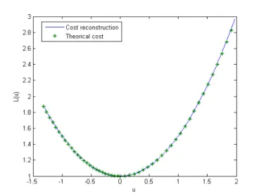
Figure 1. Ideal reconstruction
Figure 2. Reconstruction (left) on the basis of two experiments from a pilot (right).
Figure1shows just reconstruction based upon perfect experiments, computed from the known cost. Of course, this is just checking that the theory is not false, and that no purely numerical problem appears. This last point is not so obvious, as explained just below.
On the other hand, experimental data were obtained from the simulator (developed in our project) [2] in its manual mode. Datas shown here, in Figure 2 come from a beginner pilot. The pilot was just asked twice to change from flying direction for a parallel one, which implies the existence of an inflexion point (zero curvature). For the sake of testing the algorithm performances, we considered minimum possible level of information, i.e., two trajectories only. Both trajectories were restricted to the maximum monotonicity interval.
One can see that, in this type of experiment (change for a parallel way), monotonicity looks not satisfied (it is very close not to be, and here, there is a real sensitivity problem in practice). Two costs have been reconstructed from the determination of both adjoint vectors, obtained from least squares.
One can see that this pilot actually looks to minimize a cost of the requested form, and this cost looks properly reconstructed (both reconstructions are very close).
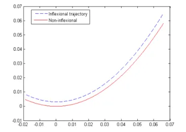
Figure3shows a reconstruction, from the same pilot, on the basis on two trajectories without inflexion points. These second experiments have been performed one month later.
Figure 3. Non-inflexional experiments, same pilot.
Figure 4. Comparison of both reconstructed criteria.
In Figure4, we show a comparison of the reconstructed criteria for the two previous couples of experiments. Of course we make the best possible fitting using our correction term L(u) = a(˜L(u) + bu). It seems that this pilot really minimized the same cost.
As a conclusion, the first trials we made seem to confirm the applicability of the method, and the reliability of the algorithm.
A measurement series with experimented pilots is on the point to be performed on their own training simu-lator.
6. Extension of the results to the case ˙q = F
0(q) + uF
1(q)
In this section, we generalize the results obtained in the previous sections to the more general class of smooth systems of the form
˙q = F0(q) + uF1(q), q∈ Q, u ∈ R, (6.1)
with the state space Q being an n-dimensional connected, Hausdorff and paracompact smooth manifold. To do so we follow exactly the same lines as in the previous sections and we do not repeat all the computations but we only point out the main differences. It is worth to notice that this case is even easier to handle.
In particular, the irrelevant linear degree of freedom in the cost L(u) disappears: as explained below, the cost is now determined up to a multiplication by a positive scalar only and a simpler normalization is now given in Lemma 6.2.
As for system (2.1), we consider the problems (PL) and ( PL ), but for the general system (6.1) now.
Similarly to Section3.1.2, we define the Hamiltonian function h(λ, p, q, u) = pF0(q) + upF1(q) + λL(u), with
p∈ Rn and λ" 0, in order to apply the PMP to Problem (P L).
Again, abnormal extremals have to be avoided, and we consider only normal extremals only, i.e., we assume that λ = −1.
All the information is still contained in the system: ⎧ ⎪ ⎪ ⎨ ⎪ ⎪ ⎩ ˙q = F0(q) + uF1(q) ˙p = −p∂F0 ∂q − up ∂F1 ∂q L∗(pF1(q)) + pF0(q) = 0. (6.2)
Using the u-parametrization of the experiments and taking into account the fact that p satisfies a linear ODE, the last equation of the previous system rewrites
L(u)− uL′(u) = p0V (u), (6.3)
where p0 is the initial value of p(·), and V (u) is defined by
p0V (u) = p(t(u))F0(q(t(u))).
Most of the material and results developed in the previous sections remain unchanged with system (1.3) replaced by system (6.1). The main change is that the criterion L(u) is now reconstructed modulo multiplication by a scalar only. Indeed, the transformation L → aL(u) + bu does not leave invariant the set of extremal trajectories, only the transformation L → aL does. For this reason, Lemmas3.14and3.15modify as follows. Lemma 6.1. Let a be a positive number and let b be real. The two optimal control problems (PL) and (PaL)
have the same set of extremal trajectories, while, in general, the two optimal control problems (PL) and (PL+bu)
do not.
Lemma 6.2. At u0, the cost function L to be reconstructed can be normalized so that L′′(u0) = 1.
Besides this, Theorem4.1 is also true for system (6.1) and its proof generalizes straightforwardly, with some extra work.
References
[1] A.A. Agrachev and Y.L. Sachkov, Control theory from the geometric viewpoint. Springer-Verlag, Berlin, Encyclopaedia of Mathematical Sciences 87 (2004). Control Theory and Optimization, II.
[2] A. Ajami, T. Maillot, N. Boizot, J.-F. Balmat, and J.-P. Gauthier. Simulation of a uav ground control station, in Proceedings of the 9th International Conference of Modeling and Simulation, MOSIM’12 (2012). To appear, Bordeaux, France (2012). [3] G. Arechavaleta, J.-P. Laumond, H. Hicheur, and A. Berthoz, Optimizing principles underlying the shape of trajectories in
goal oriented locomotion for humans, in Humanoid Robots, 2006 6th IEEE-RAS International Conference on (2006) 131–136. [4] G. Arechavaleta, J.-P. Laumond, H. Hicheur, and A. Berthoz, On the nonholonomic nature of human locomotion. Autonomous
Robots 25 2008 25–35.
[5] G. Arechavaleta, J.-P. Laumond, H. Hicheur, and A. Berthoz, An optimality principle governing human walking. Robot. IEEE Trans. on 24 2008) 5–14.
[6] B. Berret, C. Darlot, F. Jean, T. Pozzo, C. Papaxanthis, and J.P. Gauthier, The inactivation principle: mathematical solutions minimizing the absolute work and biological implications for the planning of arm movements. PLoS Comput. Biol.4 (2008) 25.
[8] Y. Chitour, F. Jean, and P. Mason, Optimal control models of goal-oriented human locomotion. SIAM J. Control Optim.50 (2012) 147–170.
[9] H. Chitsaz and S. LaValle, Time-optimal paths for a dubins airplane, in Decision and Control, 2007 46th IEEE Conference on (2007) 2379–2384.
[10] F. Chittaro, F. Jean, and P. Mason. On the inverse optimal control problems of the human locomotion: stability and robustness of the minimizers. J. Math. Sci. (To appear).
[11] J.-P. Gauthier, B. Berret, and F. Jean. A biomechanical inactivation principle. Tr. Mat. Inst. Steklova268 (2010) 100–123. [12] M. Golubitsky and V. Guillemin, Stable mappings and their singularities. Springer-Verlag, New York, Graduate Texts in
Mathematics14 (1973).
[13] F. Jean, Optimal control models of the goal-oriented human locomotion, Talk given at the “Workshop on Nonlinear Control and Singularities”, Porquerolles, France (2010).
[14] W. Li, E. Todorov, and D. Liu, Inverse optimality design for biological movement systems. World Congress18 (2011) 9662– 9667.
[15] L.S. Pontryagin, V.G. Boltyanskii, R.V. Gamkrelidze, and E.F. Mishchenko, The mathematical theory of optimal processes, Translated from the Russian by K.N. Trirogoff, edited by L.W. Neustadt. Interscience Publishers John Wiley & Sons, Inc. New York-London (1962).
[16] S.M. Rump, Verification of positive definiteness. BIT 46 (2006) 433–452.
[17] R. Thom, Les singularités des applications différentiables. Ann. Inst. Fourier Grenoble 6 (1955–1956) 43–87.