HAL Id: lirmm-00857347
https://hal-lirmm.ccsd.cnrs.fr/lirmm-00857347
Submitted on 11 Sep 2013
HAL is a multi-disciplinary open access
archive for the deposit and dissemination of
sci-entific research documents, whether they are
pub-lished or not. The documents may come from
teaching and research institutions in France or
abroad, or from public or private research centers.
L’archive ouverte pluridisciplinaire HAL, est
destinée au dépôt et à la diffusion de documents
scientifiques de niveau recherche, publiés ou non,
émanant des établissements d’enseignement et de
recherche français ou étrangers, des laboratoires
publics ou privés.
Gérard Subsol
To cite this version:
Roseline Bénière, Gilles Gesquière, François Le Breton, William Puech, Gérard Subsol. A
comprehen-sive process of reverse engineering from 3D meshes to CAD models. Computer-Aided Design, Elsevier,
2013, 45 (11), pp.1382-1393. �10.1016/j.cad.2013.06.004�. �lirmm-00857347�
Contents lists available atSciVerse ScienceDirect
Computer-Aided Design
journal homepage:www.elsevier.com/locate/cad
A comprehensive process of reverse engineering from 3D meshes to
CAD models
Roseline Bénière
a,c,∗, Gérard Subsol
a, Gilles Gesquière
b, François Le Breton
c,
William Puech
aaLIRMM, University of Montpellier 2, CNRS, 161 rue Ada, 34 095 Montpellier Cedex 5, France bAix-Marseille University, LSIS, CNRS, IUT, BP 90178, 13 637 Arles Cedex, France
cC4W, 219 rue le Titien 34 000 Montpellier, France
h i g h l i g h t s
• Primitive extraction: detect primitive which corresponds locally to the 3D mesh.
• Adjacency relation determination: define the relationship between primitives.
• Wire construction: based on the intersection curves between neighboring primitives.
• B-Rep creation: that works even in the case of an outline on a periodic surface.
a r t i c l e i n f o Article history: Received 23 December 2011 Accepted 8 June 2013 Keywords: CAD Reverse engineering 3D mesh
Boundary representation (B-Rep) 3D curvature
Geometric primitive fitting
a b s t r a c t
In an industrial context, most manufactured objects are designed using CAD (Computer-Aided Design) software. For visualization, data exchange or manufacturing applications, the geometric model has to be discretized into a 3D mesh composed of a finite number of vertices and edges. However, the initial model may sometimes be lost or unavailable. In other cases, the 3D discrete representation may be modified, e.g. after numerical simulation, and no longer corresponds to the initial model. A retro-engineering method is then required to reconstruct a 3D continuous representation from the discrete one.
In this paper, we present an automatic and comprehensive retro-engineering process dedicated mainly to 3D meshes obtained initially by mechanical object discretization. First, several improvements in automatic detection of geometric primitives from a 3D mesh are presented. Then a new formalism is introduced to define the topology of the object and compute the intersections between primitives. The proposed method is validated on 3D industrial meshes.
© 2013 Elsevier Ltd. All rights reserved.
1. Introduction
Nowadays, manufactured objects are principally designed with Computer-Aided Design (CAD) software. An object is constructed by combining geometric primitives like planes, spheres, cylinders, cones or parametric patches (e.g. Bezier, B-Splines, NURBS) and their boundaries (using intersections between primitives). This continuous representation is necessary to redesign or extract the object parameters. However, many CAD design software programs do not read or write opened geometric formats like STEP or IGES, e.g. the basic version of AutoCAD can only store a model in its proprietary format (DWG). Furthermore, for visualization,
∗Corresponding author at: LIRMM, University of Montpellier 2, CNRS, 161 rue
Ada, 34 095 Montpellier Cedex 5, France. Tel.: +33 4 67 41 85 65.
E-mail addresses:[email protected],[email protected]
(R. Bénière),[email protected](G. Subsol),[email protected]
(G. Gesquière),[email protected](F. Le Breton),[email protected](W. Puech).
exchange or manufacturing purposes, the continuous parametric CAD model must be discretized into a 3D CAD mesh composed of a finite number of vertices and triangles. The initial CAD parametric data may be unavailable, lost or no longer correspond to the original CAD model if the 3D mesh is deformed by another designer or after a numerical simulation process. For example, inFig. 1, a B-Rep model was discretized into a 3D mesh in order to be deformed by a stamping simulation tool. But a continuous model is often required to check the shape parameters or to modify the design. Reconstruction of a B-Rep model from the modified 3D CAD mesh, which is a particular case of reverse engineering, is thus needed.
In our industrial context, we work in collaboration with the C4W1company. Through the user tests of 3D Translate,2a software
1 www.c4w.com. 2 www.3dtranslate.com/. 0010-4485/$ – see front matter©2013 Elsevier Ltd. All rights reserved.
Fig. 1. The B-Rep model has to be discretized into a 3D CAD mesh in order to be processed by a metal press stamping die parts simulation, and no longer correspond with the
final mesh.
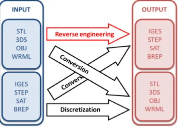
allowing interoperability between CAD software translating or converting many file formats (seeFig. 2), we note considerable interest in reconstructing continuous models from 3D CAD meshes. In fact, around 90% of requests concern obtaining a continuous representation (IGES, STEP, etc.) from a 3D mesh (STL, OBJ, etc.), of which 50% are CAD meshes. A specific method, focused on reconstruction from meshes created by CAD model discretization, is thus required.
The reverse engineering process has to be adapted to the 3D mesh structure, which depends on the creation or discretization process. For example, for a scanned physical object, the 3D mesh is generally very dense but composed of points whose coordinates may be disturbed by acquisition noise. On the other hand, dis-cretization of a CAD model has accurate points but the mesh can be sparse because the discretization function does not add useless points. So, between a scanned mesh which contains many noisy points and a CAD mesh with few points but with exact positions, the reconstruction process may differ. The CAD model reconstruc-tion problem corresponds to the second case and is rarely pre-sented in the literature. Indeed, most reverse engineering papers try to reconstruct continuous objects from a scanned mesh. These methods cannot be used on a sparse mesh and a dedicated algo-rithm has to be developed.
We can distinguish, as in [1], two kinds of reverse engineer-ing results: ‘‘simple surfaces’’, such as planes, and general ‘‘free-form surfaces’’, like B-Splines or NURBS. For the second case, many methods to fit free-form surfaces on a 3D mesh exist, for exam-ple [2]. Although they are efficient for obtaining a good-looking re-construction of a 3D mesh and allow modeling of some features (see for example [3,4]), they do not reveal the overall information on the shape that is essential for many CAD applications. In partic-ular, the identification of the object shape (a sphere or plane?), the computation of shape parameters (e.g. a radius or an axis of revo-lution) or the definition of relationships between different parts (a cylinder linking two tangent planes can be considered as a blend) are not possible with these methods.
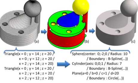
Furthermore, in the CAD model, the primitives are confined by boundaries defined as parametric 3D curves. So a CAD model reconstruction process should extract primitives, like planes, spheres or cylinders, then it has to compute their boundaries and relations so as to construct a topologically-consistent continuous CAD model (seeFig. 3).
We decided to use the Boundary Representation (B-Rep) to store the CAD model (more details can be found in [5]). This repre-sentation allows us to study or modify the object after conversion using C4W software: 3D Shop,3and it is also easy to stock it in a common format such as IGES or STEP.
In a B-Rep model (Fig. 3(c)), an object is represented by a set of faces. Each face corresponds to a geometric primitive defined by its parameters (e.g. a radius and a center in the case of a sphere) and its boundaries, or so-called wires: one exterior for the outer boundary and eventually one or several interior ones for the hole boundaries. A wire is made with one or several edges which are defined by a
3www.c4w.com/dev/?lang=en#customcad.
Fig. 2. 3D Translate software schema.
parametric equation and two limit points. These edges correspond to parts of intersections between two faces. In particular, if two faces are neighbors, their wires will reference common edges. Then the B-Rep model construction requires not only recovery of the primitive set, but also all the adjacency relations between the faces, in order to create topologically-consistent wires.
In this paper, we present a comprehensive method to recon-struct a B-Rep model composed of planes, spheres, cylinders and cones from a 3D mesh whose vertex coordinates are considered exact. After presentation of the state of the art in Section2, our method is detailed in Section3. The CAD object results are pre-sented in Section4. The method is discussed along with its per-spectives in Section5.
2. State of the art
In this section, a study of several methods is proposed. The first part is dedicated to comprehensive procedures for reconstructing continuous objects but there are few. So in the second part, papers dealing with only one part of the procedure will be studied. The method proposed in this paper has three steps, the primitives are extracted first, then the wires are computed and the B-Rep model is then constructed. So methods proposing solutions to detect and reconstruct primitives and to compute the adjacency relations and the boundaries are analyzed.
2.1. Complete procedure
Many papers deal with part of the B-Rep reconstruction process but very few describe a complete procedure. A first one was pro-posed by Benko et al. in [6]. They begin the reconstruction pipeline by a segmentation step.
For each sub-mesh, the authors do not extract the geometric primitive type but instead they conduct many approximation tests to fit a parameterized geometric primitive. This method can con-fuse the primitive type, and indeed in the example given in the pa-per, cylinders are not detected as cylinders but rather as parts of
Fig. 3. From a 3D mesh to a B-Rep model.
a revolution surface. This confusion does not block the reconstruc-tion but it does not allow extracreconstruc-tion of all of parameters such as the cylinder radius. Then the topology is computed using a 3D mesh: two primitives are adjacent if the corresponding sub-meshes share at least one mesh edge. The wire construction is based on these common edges and is refined by the exact geometric intersection computation. In fact, this method depends on the edge accuracy and gives interesting results only if the 3D mesh is dense and if the mesh edges correspond to the continuous boundaries of the real object. Furthermore, the vertex normals are used to segment the mesh and to compute certain primitive parameters using a Gaus-sian sphere, while the computation of accurate normals requires many points or points without noise. Thus the authors did not di-rectly use the object of the Hoschek benchmark as an example but they redesigned and resampled it.
Huang and Menq [7] propose a process to reconstruct a B-Rep model from a 3D point cloud. The first step consists of triangu-lating the point cloud. Then the authors propose to segment the mesh by using border edge detection and compute the primitive parameters for each sub-mesh with a method based on surface normal estimation. The topology is deduced from the sub-meshes as in [6]; the common mesh edges give the adjacency relationship and allow construction of a first approximation of wires. Huang and Menq replace all the common edges by the real intersection curves between the corresponding faces. The resulting quality of this method is also related to the 3D mesh edge accuracy. Further-more, it is not possible to construct a wire if four or more primitives have the same intersection point that limits the reconstructed CAD model complexity.
Recently, Chang and Chen [8] proposed a review of reverse en-gineering methods. In particular, they analyze some commercial software, like Geomagic Studio or Rapidform XOR. They show, as in [1], that two kinds of results can be found. In the case of free-form surfaces (generally based on NURBS), commercial software propose automatic methods that are efficient but some problems remain when dealing with objects with sharp edges. Although all of these software packages also include some methods to reconstruct a CAD model based on geometric primitives, they do not work au-tomatically, mostly if the 3D mesh has some sparsely discretized parts. The user has to interact by clicking along the boundaries or defining the type of primitive for each mesh part; thus a complex object reconstruction can take several hours or days. These meth-ods are thus not available for industrial applications, unlike the process presented in this paper.
2.2. Detection and reconstruction of primitives
In recent years, many methods have been proposed to extract only geometric primitives in a reverse engineering process. They generally involve three steps [1]: point area extraction which de-fines mesh areas having the same shape features; classification which associates one primitive type with each point area and the fitting to compute primitive parameters corresponding to each point area. Thus, in the method proposed by Benko et al. [9], the shape features are based on co-planarity between neighbor trian-gles. They highlight the sharp edges or small blends which sepa-rate the sub-meshes. Then a plane is fitted to each sub-mesh. If the plane is close enough to the sub-mesh, it is kept. Otherwise, the sub-mesh is approximated with more complex geometric primi-tives such as a sphere, cylinder, etc., until it closely corresponds. Note that the authors do not formally classify the geometric prim-itive type but test all possibilities and, as we have already said, this method can lead to confusion between types. This fitting re-sult may be improved by adding some constraints such as tangency between the geometric primitives. In [10], Bénière et al. propose to use curvatures to segment the mesh, to define the primitive kind associated with each sub-mesh and to compute the primitive pa-rameters.
Many papers deal with just one step. For example, Bohm et al. [11] and Lavva et al. [12] describe techniques to segment and classify the sub-mesh by using curvature features. The segmenta-tion is based on propagasegmenta-tion from a seed triangle to triangles with the same curvature feature. In a second step, using curvature prop-erties of the geometric primitives, a type is attributed to each sub-mesh. Sunil and Pande [13] base the segmentation and classi-fication steps on the CAD mesh characteristics. The dihedral angle and the size of each triangle are used for segmentation. A first clas-sification is made with the curvature feature and then, with CAD
a priori knowledge, the sub-meshes can be further classified. For
example, if a cylinder is between two planes, it corresponds to a blend.
Lukács et al. [14], Shakarji [15] and Schnabel et al. [16] propose solutions to only fit primitives on a sub-mesh or a point cloud. Lukács and Shakarji’s methods use two kinds of approximation on all points to obtain the primitive parameters. In contrast, Schnabel et al. define one primitive for each point group (e.g. groups of three points for a plane) and keep the best one. The Chaperon and Goulette method [17] is more specific and deals only with point cloud approximation by a cylinder. This approximation is based on features of the cylinder Gaussian image. The Gaussian image of a
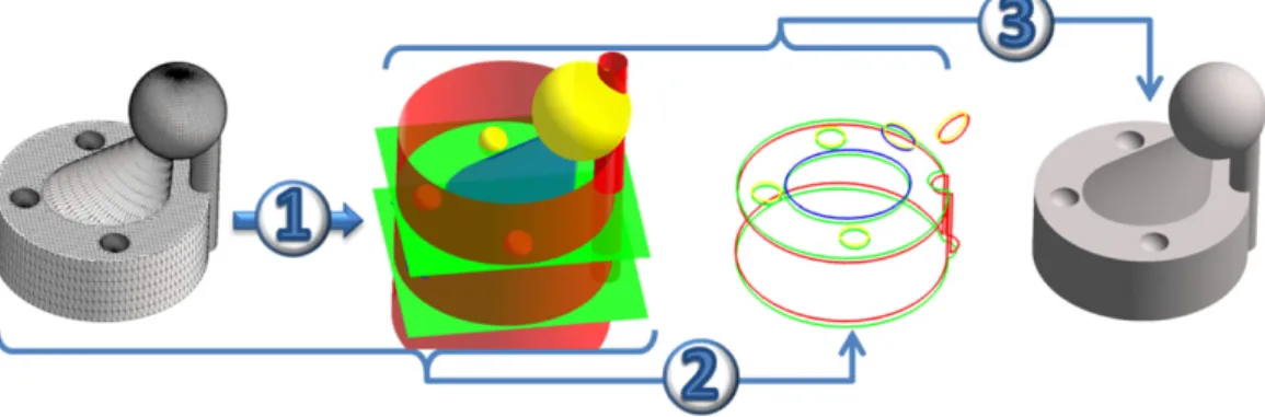
Fig. 4. Overview of the reverse engineering method: Step 1: primitive extraction, Step 2: wire construction and Step 3: B-Rep creation.
cylinder gives the axis and, in case of cones, this gives the angle too.
Even though these methods give good results, their adaptation is not always possible in a complete process. However, some of the ideas were adopted for our method.
2.3. Adjacency relations and boundaries
Adjacency relations between the geometric primitives which are extracted from a mesh are important in many domains. Thus, in [18], Li et al. use these relations to align primitives after a RANSAC extraction. The authors construct a graph to represent the relation between primitives, and to extract primitives connected by the same feature. In this article, the extracted relations are not adjacency relations but rather relations on primitive parameters, like the same axis, or the same radius. In contrast, in [19], adjacency relation extraction allows remeshing improvement. Chappuis et al. [19] use relations between primitives to construct correct intersections and to be sure that the edges corresponding to these intersections are not deleted by this remeshing. After computation of primitives belonging to the mesh, the adjacency relations are extracted from the sub-meshes used to compute the primitives and are stored in an adjacency graph. The intersections between primitives which guide the remeshing are computed using this graph defined by a primitive node and an edge if the primitives are neighbors. Even though this is not a B-Rep reconstruction method, its definition of the relationship between faces can be used to extract consistent intersections and reconstruct a B-Rep model.
Computing intersection curves between two geometric prim-itives is a classical problem and efficient methods exist (see for example [20]). The difficulty is in combining parts of these inter-section curves, computed on pairs of geometric primitives, in con-sistent wires that are continuous and closed curves.
This seems very similar to the so-called ‘‘Boundary Evalua-tion’’ [21] problem which allows recovery of a B-Rep representa-tion from a CSG model. For example, Miller [22] first computes intersections between all solids. Indeed, in the case of a CSG, the primitives are solid, for example a cylinder is described by a cylin-drical surface and by the two extreme circular planes. Miller then gets a set of edges which are labeled as Cross-edge for an edge resulting from an intersection or Self-edge for an edge already ex-isting in the CSG model. The wire construction is based on the defi-nition of a path through the edges; if several paths are possible, the path using the Cross-edge is chosen. Thus the wires are constructed for each face with intersections between the volumes. Neverthe-less, the Boundary Evaluation problem is much easier because it is based on an exact set of bounded volume primitives, whereas in our case only infinite surface primitives associated with a discrete set of points are used.
3. Towards a new B-Rep reconstruction process
3.1. Overview of our method
Our comprehensive process, presented in this section, involves three steps (seeFig. 4):
•
Step 1: Primitive extraction: in this step, the idea is first to detectthe type of geometric primitive (i.e. a plane, sphere, cylinder or cone) that corresponds locally to the 3D mesh and to then compute the parameters which give the best fit. The method is based on differential geometry operators which characterize the local 3D shape.
•
Step 2: Wire construction: this is a key complex problem. Itdefines the relationship between all the extracted geometric primitives, which is subsequently used to compute intersection curves between two geometric primitives. Then all of these curves are combined to build a continuous wire in a consistent way.
•
Step 3: B-Rep creation: the B-Rep construction is presented.It consists of combining the information extracted or recon-structed during the two previous steps to construct a consistent model.
3.2. Step 1: primitive extraction
The local shape around point P on a surface S is characterized by the minimum and maximum principal curvature (kminand kmax)
and by the two principal directions (dminand dmax) corresponding
to the tangent vectors for which the principal curvatures are obtained. Simple geometric primitives, like planes, spheres, cones and cylinders, have specific curvature characteristics (seeTable 1). Thus, in the case of a plane, the curvature value is equal to 0, which means kmin
=
kmax=
0. For a sphere, all the points have thesame curvature whose value is equal to the inverse of the radius (kmin
=
kmax=
1R). A cone or a cylinder point is characterizedby one principal curvature equal to 0 with the corresponding principal direction following the cone or cylinder generating line. Furthermore, the other principal curvature allows us to define a point on the axis for each point on the cone or cylinder.
The first step of the method (see [10]) extracts primitives from a 3D mesh using these curvature characteristics. Therefore for the mesh inFig. 5(a), the curvature is computed and displayed on the mesh ofFig. 5(b) with a color code: green for planar, yellow for spherical, blue for convex and red for concave points.
Many methods have been proposed to compute the curvature on a discrete 3D mesh as reviewed in the surveys [23,24]. In the following, a combination of the two methods described in [25,26] is used. The idea proposed in these papers involves computing, for each neighbor vertex, a discrete curvature; using a regression based on the Euler formula, the principal curvatures are obtained.
Table 1
Curvature features for each primitive type.
kmin kmax dirmin dirmax
Plane =0 =0 Not defined Not defined Sphere =Rayon1 =Rayon1 Not defined Not defined Cone/cylinder =0 =
1
dist(Point,Axis) =generating line Not used
= 1
dist(Point,Axis) =0 Not used =generating line
Fig. 5. (a) Original 3D mesh, (b) Curvature parameter computation: planar point (green), spherical point (yellow), convex point (blue) and concave point (red), (c) Point
areas, (d) Extracted geometric primitives. (For interpretation of the references to colour in this figure legend, the reader is referred to the web version of this article.)
Then, using the curvature features, point areas are extracted with a propagation method and labeled (Fig. 5(c)) by one color per primitive type. To offset the numeric noise or irregularities in the
point area extraction, epsilons, computed according to the input
mesh, are used. The parameters of one primitive are approximated for each point area, with linear approximation and curvature verification; the extracted primitives are shown inFig. 5(d).
3.2.1. Plane and sphere extraction
To find planes and spheres, neighbor vertices having
|
kmax−
kmin|
< ϵ
SP are grouped in the same point areas. A point area is initialized by a first point and propagated to the neighbor points having the same curvature characteristics. Then, for each pointarea, a geometric primitive is fitted. If
|
kmax+kmin2
|
< ϵ
PL, the point area corresponds to a plane. The implicit Eq.(1)is used to extract coefficients by linear regression.ax
+
by+
cz+
d=
0.
(1)If
|
kmax+kmin2
|
> ϵ
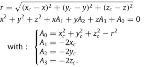
PL, the point area corresponds to a sphere. Theimplicit Eq.(2)of the sphere is not linear and not easy to fit by the least-squares method. So, the center and the radius of the sphere are approximated using Eq.(3)obtained by a variable change [27]. A regression with a least-squares method is also carried out in this case. r
=
(
xc−
x)
2+
(
yc−
y)
2+
(
zc−
z)
2 (2) x2+
y2+
z2+
xA1+
yA2+
zA3+
A0=
0 with:
A0=
x2c+
y 2 c+
z 2 c−
r 2 A1= −2x
c A2= −2y
c A3= −
2zc.
(3)3.2.2. Cone and cylinder extraction
A cylinder is considered to be a particular case of a cone. These primitives are characterized by two 3D lines: the rotation axis and the generating line. The axis is defined by a vector and a point which is the cone vertex or any axis point for cylinders. The generating line can be determined by the angle to the rotation axis in the case of a cone or by the radius for a cylinder. Both geometric primitives have the same curvature behavior: kmin
=
0,
dmincorresponds to the generating line and the point P
+
n·
1kmaxbelongs
to the rotation axis, with P being a point on the cone and n the normal in P.
Fig. 6. A key criterion to check if two neighbor points belong to the same cone or
cylinder:α1=α2.
In the other methods, detection of cones or cylinders using curvature features is only based on the curvature values: one equals 0 and one differs from 0. Although the points on cones or cylinders have this property, some points on other primitives can have the same property like certain ruled surfaces. Here we define a new criterion to exclusively detect cone or cylinder points. Thus to check if two neighbor points belong to the same cone or cylinder, the following key criterion is used (seeFig. 6). Let P1′
=
P1+
n1·
1 Cur1and P2 ′
=
P2+
n2·
1 Cur2,
P1 ′and P2′define a potential axis A and
(
P1,
d01)
and(
P2,
d02)
define two potential generating lines.P1 and P2 belonging to the same cone or cylinder must satisfy:
the angles
α
1 andα
2 between axis A and the generating lines are identical (and close to 0 in the case of a cylinder).This criterion is used to extract point areas corresponding to cones or cylinders. If two neighbor vertices have a kmin
< ϵ
Coand kmax> ϵ
Co, they belong to a cone. Then the criterion is used, toensure that they belong to the same cone. Secondly, to propagate the point area, the curvature of the neighbors is also studied to check the criterion with these vertices.
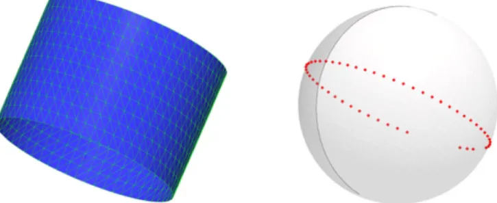
For each point area, a cone or cylinder is approximated by using the Gaussian image and not only the property of the curvature as in [10]. In the case of cones or cylinders, the Gaussian image
Fig. 7. A cylinder and its Gaussian image. All points of the cylinder are projected
onto a circle.
is a circle (seeFig. 7). The normal of the plane which fits this Gaussian image corresponds to the direction of the axis. It allows us to obtain the axis and also the angle for the cone. To determine the cylinder radius, the points of the point area are projected onto the approximated plan and form a circle which corresponds to a cylinder circle, i.e. with the same radius and the center equivalent to an axis point.
3.2.3. Improving computation of the curvature by a pre-segmentation step
Curvature computation is based on the vertex neighborhood. In the case of a sparse mesh, the vertices can correspond to several primitives because only the points on the object edges are used. For these meshes, if the edges of the object are detected and used to make a segmentation, a vertex on an edge will belong to several sub-meshes. Computation of the curvature is thus better with segmentation; with the neighborhood of each vertex not being disturbed by vertices of other primitives. In our case, the dihedral angle (angle between two triangles) is used to obtain this pre-segmentation by a propagating method. After initialization with a not yet used triangle, the neighbor triangles are added to the sub-mesh, if the dihedral angle between its and the neighbor triangle belonging to the sub-mesh is greater than a threshold angle. This segmentation improves our primitive extraction. In
Fig. 8, the point areas (Fig. 5(d)) extracted from the segmented meshes (5(b)) are more extended than the point areas obtained from the original mesh. In other cases, no primitives are found without this segmentation, whereas with the segmentation all primitives are detected and reconstructed.
3.3. Step 2: wire construction
3.3.1. Building an adjacency relationship graph
In order to get a B-Rep representation, each geometric primitive has to be trimmed, according to its intersections with the other ones. To find out which intersection is involved to build the wires, the adjacency relations are determined. An adjacency graph containing the relationship between the primitives is used for this purpose. Each primitive corresponds to a node of the graph, and an edge is added between two nodes if the two corresponding primitives are neighbors.
The extraction of point areas is based on a propagation method. A point area is initialized by a vertex with specific curvature and neighbor vertices with the same curvature characteristics (according to the primitive type) are added to the area. During this construction, vertices on the primitive limits cannot be added in the point area. Indeed, the curvature computation is based on a neighborhood study for each vertex, so the vertex curvatures on the primitive limits are disturbed by the vertices of the neighbor primitive. To obtain point areas containing all vertices corresponding to the primitive, an extension of these areas is then carried out. To extend a point area, the distance between adjacent
Then, the extended areas allow us to define the common points (Fig. 9(b)). For each pair of primitives, a set of common points is defined; if a point belongs to several extended areas, it is added to the common points of the primitive pair corresponding to the extended areas. An adjacency graph is used to represent the adjacency relations. It is initialized with a node by primitive. If the set of common points corresponding to two primitives is not empty, an edge is added to the graph between the two corresponding nodes, as shown inFig. 9(c).
3.3.2. Extracting valid intersection curves for our wire construction
In the first step, no limit is defined for the geometric primitives, and they can be infinite as planes, cylinders or cones. To recover
wires representing the geometric primitive boundary, the
intersec-tion curves between the geometric primitives first have to be com-puted.
For this, the edges of the adjacency graph which define pairs of intersecting primitives are used. We decided to use the Open
Cascade Library4 to perform this operation which gives
inter-section curves as parametric curves which can be closed (e.g. sphere/plane) or infinite (e.g. plane/plane). These parametric curves are defined by an equation according to the type (a B-Spline curve or a circle, for example) and two limit points.
InFig. 9(d), the set of all intersection curves between geometric primitives is presented. However, the problem is not very straightforward, some intersection curves are not really significant such as the one between the cylinder Cyl2 and the top of the sphere Sph1. Then the validity of each intersection curve has to be checked by comparing it with the common points shared by the two corresponding primitives. Then, inFig. 9(e), the red intersection curve is rejected whereas the green ones are validated.
3.3.3. Decomposing intersection curves into edges
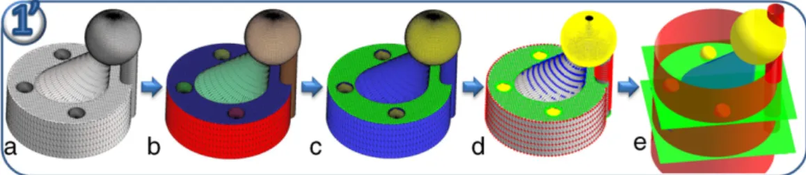
The geometric primitives do not only intersect two by two. For instance, inFig. 9(e), the side cylinder Cyl2 intersects, at the same location, the superior plane Pl1 and the main cylinder Cyl1. In this area, the contour of Cyl2 will then be composed of portions of the two intersection curves with Pl1 (a circle) and Cyl1 (two parallel lines). More generally, each valid intersection curve has to be decomposed into parts corresponding to the intersection restricted only to two primitives. These parts are called edges and are delimited by junction vertices which correspond to intersections between three geometric primitives.
The example inFig. 10is used to explain the edge construction. From the mesh inFig. 10(a), fourteen planes are extracted and the
adjacency graph is deduced, seeFig. 10(b). Intersection curves are computed for each primitive pair bound in the graph,Fig. 10(c).
First, all potential junctions are extracted by intersecting all valid intersection curves two by two. Nevertheless, not all the potential junctions are valid: they have to correspond in the B-Rep model to a vertex, i.e. to a connection between two edges, so it binds three primitives as shown inFig. 10(a). Furthermore, these three primitives have to be adjacent two by two because they have a common vertex. This implies that the four geometric primitives leading to the junction (two per valid intersection curve) are in fact three (one in common on the two edges) and that they are connected, forming a cycle in the adjacency graph. As the same
junction can be extracted from several intersection pairs, a fusion
is performed when two junctions correspond to the same vertex.
Fig. 8. (a) Original 3D mesh, (b) Segmented meshes, (c) Curvature on segmented meshes, (d) Point areas on segmented meshes and (e) Extracted primitives from segmented
meshes.
Fig. 9. (a) Extended areas based on Point areas and primitives, (b) Common points, (c) Adjacency graph (one node per primitive and an edge if the two primitives are
adjacent), (d) Intersections between adjacent primitives, (e) Intersections validated (in green) or rejected (in red) with the common points, (f) Edges, (g) wires assembled using the extended areas and (h) the reconstructed B-Rep model. (For interpretation of the references to colour in this figure legend, the reader is referred to the web version of this article.)
After the junction extraction and fusion, the edges are created by cutting the valid intersection curves. To construct the wires, a closed path through the edges is constructed; so if an edge has an extremity which is not connected with an another edge extremity, this edge cannot belong to a closed path. All of these edges are removed. Thus a set of valid edges is obtained, as shown inFig. 11.
3.3.4. Assembling edges to build wires
To build wires, one exterior and zero or several interior ones for each geometric primitive, closed paths have to be computed that assemble a subset of the valid edges. In fact, there are two cases: a
wire can be created in an unique way with the valid edges or several
Fig. 10. (a) 3D mesh, (b) Extracted geometric primitives (14 planes in this case) with the overlapped adjacency graph and (c) Valid intersection curves.
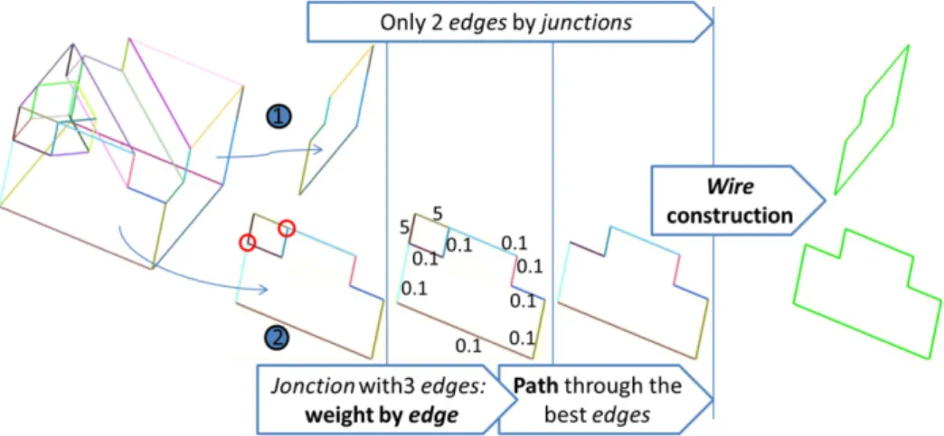
Fig. 11. Case 1: one way to assemble edges into a wire. Case 2: several possible paths, allocating weights to the edges and minimizing the total weight of the path; a wire is
built in a non-ambiguous way.
In the first example inFig. 11, the seven valid edges are available for the frontal plane of the object. All of these edges are connected two by two, and there is only one way to make a closed path. In this case, building the wire is straightforward. In the second example in
Fig. 11, several closed paths are possible: one follows the exterior boundary or a second shortcuts the corner or a third just with the corner.
To choose between the different paths, a weight is attributed to each edge. This weight corresponds to the average distance between the edge and the extended areas. The minimal distance induces the most probable edge on the object. A sequential method is used to find a path closer to the optimal path. The wire construction is initialized with the edge having the lowest weight. Then the connected edges are studied and the one with the lowest weight is selected and connected to the current wire. The process terminates when the wire is closed or if there is no more edge to connect. The wire is kept in the first case but rejected in the second. In Fig. 12, all wires computed from the mesh ofFig. 10are presented. This building process ensures that all wires have a valid topology. They are closed and cannot self-intersect (otherwise there will be a supplementary junction on the self-intersection). After the B-Rep creation, the consistency of the wire can be checked by assessing whether the B-Rep model is closed: all faces are entirely delimited by the edges.
3.4. Step 3: B-Rep model creation
Once the wires have been constructed, they are combined with the geometric primitives and the adjacency graph to reconstruct the B-Rep model (seeFig. 9(h)).
The B-Rep model is composed, for each geometric primitive, of its type of primitive, its parameters, and the corresponding wires, i.e. one outer and no or several inner ones for the hole boundaries. Each edge is stored once and the wires only reference the edges. This structure ensures that the model is watertight because the adjacent faces have edges in common, unlike a structure in which each boundary is defined without links with the others.
Fig. 12. Valid edges are consistently assembled to create wires of the 3D mesh in
Fig. 10.
4. Experimental results
The method was implemented in the 3D Shop software package produced by the C4W5company. The program only requires use of a set of some parameters. These parameters could be defined au-tomatically according to the mesh characteristics (e.g. proportional to the maximal or mean edge length) and its type (discretized CAD model or 3D scan). Our process runs entirely automatically and there is no interaction with the user. In the next section, some val-idation experiments based on several examples will be proposed.
4.1. Tests on typical meshes
The first tests are performed on CAD meshes, with a low den-sity of points but with different complexity. For these examples,
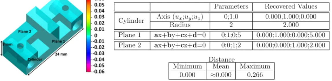
Fig. 13. B-Rep reconstruction for PlanesAndCylinders: (a) 3D mesh: (358 vertices and 736 triangles), (b) Extracted geometric primitives (6 cylinders and 16 planes),
(c) Reconstructed wires and (d) the final B-Rep model.
Fig. 14. Comparison between the recovered parameters and the initial values of the geometric primitives.
Fig. 15. B-Rep reconstruction for Tree: (a) 3D mesh: (966 vertices and 1928 triangles), (b) Extracted geometric primitives (1 cone, 6 cylinders and 71 planes), (c) Reconstructed
wires and (d) the final B-Rep model.
B-Rep models are created and discretized, to compare the result parameters with the initial parameters. The first one (seeFig. 13) contains planes and cylinders, and the 3D discretization is very sparse, with very few points. In this case (seeFig. 13(b)), all prim-itives are extracted, using the pre-segmentation step described in Section3.2.3. After the computation of wires (seeFig. 13(c)), the B-Rep model is reconstructed (Fig. 13(d)).
In Fig. 14, a quantitative analysis of the reconstruction is presented. First, the parameters of the geometric primitives are compared with those recovered by our algorithm. The values are extremely close. Then the distance between the initial 3D mesh and the B-Rep model is computed. For this, the resulting B-Rep is discretized very densely and the distance between these points and the studied mesh is computed. For the mesh, the mean distance is very low. The maximum distance could appear quite long (0.266 mm) even if it remains very short with respect to the total length of the object. But the maximal error is located along the edges and we can conclude that this is mainly due to the discretization process, which generates minimal errors on planar parts and maximal error on salient parts, and not from the reconstruction method itself.
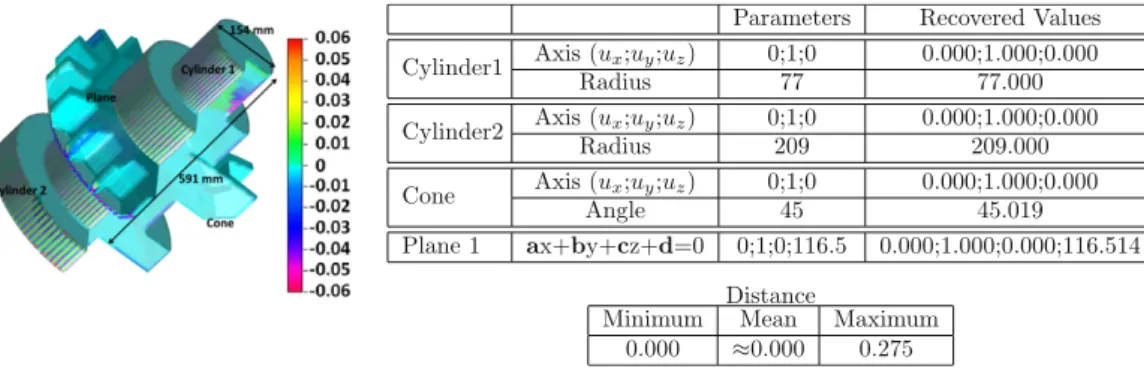
The method is also tested on more complex CAD meshes, with many intersections between more than two geometric primitives (e.g. 1 cone and several planes inFig. 15). This implies that the wires are constructed with many assembled edges that require computation of many paths to find the minimal weighted one. A sparse discretization is also chosen for this test mesh (see
Fig. 15(a)).
The reconstruction process gives very good results. The pre-segmentation step allows us to recover the 78 geometric primitives (1 cone, 6 cylinders and 71 planes) with a maximum error of 0.275 mm but corresponding to the discretization error (see
Fig. 16), whereas the mean error is close to 0. Then the wires are extracted (seeFig. 15(c)) even in complex cases, e.g. with the large plane linked to 16 other primitives (9 planes, 6 cylinders and 1 cone).
4.2. Tests on real CAD meshes
A second set of tests is performed on two real CAD objects: a cylindrical adaptor and a plate which are parts of the I4L parallel robot designed at LIRMM [28] (seeFig. 17). The CAD model was designed and discretized using Solidworks 2010. Note that the resulting 3D meshes are very sparse and irregular, which is typical of the discretization of the CAD representation of a manufactured object. The initial parameters are known and can be compared to the recovered values to assess the accuracy of the method.
The reconstruction method is applied to these meshes and gives the B-Rep models presented inFigs. 18and20. InFig. 19, the very high accuracy for all the recovered primitives is highlighted. These two real examples show the importance of the pre-segmentation step to obtain accurate results for sparse meshes.
4.3. Analysis of the computation time
The method was tested on a standard computer with an Intel
Fig. 16. Comparison between the recovered parameters and the initial values of the geometric primitives.
Fig. 17. Photographs of the cylindrical adaptor and the plate, which are parts of a
parallel robot [28].
Table 2
Computation time (Intel Core 2 Duo 2.33 GHz processor, 4 Gb RAM). Mesh Nb of triangles Nb of primitives Time
PlanesAndCylinders
(Fig. 13)
736 22 3 s
Tree (Fig. 15) 1928 78 1 m 32 s
Cylinder adaptor (Fig. 18) 540 10 1 s
Plate (Fig. 20) 3220 39 2 s
is presented inTable 2for the different 3D meshes. The computa-tion time does not only depend on the number of triangles. Thus, the reconstruction takes more than 1 min for the Tree mesh which is very small with only 1928 triangles, whereas it lasts only 2 s for the Plate mesh, which consists of 3220 triangles.
In fact, the computation time is related to the number of geometric primitives (only 39 for Plate and 78 for Tree). However, it also heavily depends on the wire number and complexity. For example, reconstruction of the PlanesAndCylinders mesh (736 triangles, 22 geometric primitives) takes much more time than for the Plate mesh (3220 triangles and 39 geometric primitives). But in this case a weight has to be computed for each edge and the best path is then extracted. We conclude that the operations which
most influence the computation time are the topology creation and the wire construction.
The objectives set by our industrial framework are clearly fulfilled.
5. Conclusion and perspectives
After a user request study in an industrial context, we concluded that the specific application of reverse engineering 3D CAD meshes has been studied very little. In this paper, a comprehensive process for automatic reconstruction of a continuous B-Rep model from a discretized 3D CAD mesh is proposed. This method involves three steps: the extraction of geometric primitives, which works successfully, unlike many existing methods, in the case of sparse meshes, by using an adapted pre-segmentation step; wire construction, which computes intersection curves between primitives in a consistent way by using a new formalism based on adjacency graph and model creation which combines all results to build a B-Rep representation.
This method gives good results with CAD meshes, indepen-dently of the mesh structure, which can be dense or sparse, reg-ular or not and even if there are many geometric primitives. This method could then be used in industrial applications, as outlined in the introduction.
Nevertheless, geometric primitives are currently limited to planes, spheres, cones and cylinders, which are very commonly used in CAD. The extraction can be improved by introducing more primitives such as ruled surfaces [29] or tori [12]. The process stays the same for these primitives: detection is done using curvature features and the parameters are computed with approximation and verified by the curvature. Then the topology reconstruction does not have to be changed to integrate these new primitives because the process is not based on the primitive type. For example, if we want to extend your method to deal with tori, we can use it to extract point areas, specific curvature features such as all points share a common principal curvature corresponding to the minor radius and the second principal curvature can be used to find the major radius and the center. Then a torus can be
Fig. 18. B-Rep reconstruction for CylindricalAdapter: (a) 3D mesh: (268 vertices and 540 triangles), (b) Extracted geometric primitives (3 cylinders and 7 planes),
Fig. 19. Comparison between the recovered parameters and the initial values of the geometric primitives.
Fig. 20. B-Rep reconstruction for Plate: (a) 3D mesh: (1585 vertices and 3220 triangles), (b) Extracted geometric primitives (21 cylinders and 18 planes), (c) Reconstructed
wires and (d) the final B-Rep model.
approximated for each extracted point area and the parameters can be verified with the curvature features.
Our method can be easily adapted to deal with fillets or blends thanks to the adjacency graph. Indeed, after an identification step during primitive extraction, the edge of the adjacency graph can be labeled to indicate the blend or fillet presence. With this infor-mation, a blend or a fillet could be added between the two linked primitives by the labeled edge, during the B-Rep construction.
Another major improvement could be to fit general parametric surfaces such as B-splines or NURBS on parts which cannot be represented by geometric primitives. In particular, this will allow management of the complex shape of blends which are very common in CAD objects.
References
[1]Várady T, Martin R, Cox J. Reverse engineering of geometric models—an introduction. Computer-Aided Design 1997;29(4):255–68.
[2]Eck M, Hoppe H. Automatic reconstruction of B-spline surfaces of arbitrary topological type. In: Proceedings of the 23rd annual conference on computer graphics and interactive techniques. ACM; 1996. p. 325–34.
[3]Vergeest JSM, Horváth I, Spanjaard S. Parameterization of freeform features. In: SMI 2001 international conference on Shape modeling and applications. IEEE; 2001. p. 20–9.
[4]Langerak TR. Local parameterization of freeform shapes using freeform feature recognition. Computer-Aided Design 2010;42(8):682–92.
[5]Stroud I. Boundary representation modelling techniques. Springer; 2006.
[6]Benkö P, Martin R, Várady T. Algorithms for reverse engineering boundary representation models. Computer-Aided Design 2001;33(11):839–51.
[7]Huang J, Menq C. Automatic CAD model reconstruction from multiple point clouds for reverse engineering. Transactions of the ASME 2002;2:160–70.
[8]Chang K, Chen C. 3D shape engineering and design parameterization. Computer-Aided Design 2011;5(8):681–92.
[9]Benkö P, Kós G, Várady T, Andor L, Ralph RM. Constrained fitting in reverse engineering. Computer Aided Geometric Design 2002;19(3):173–205.
[10]Bénière R, Subsol G, Gesquière G, Le Breton F, Puech W. Recovering primitives in 3D CAD meshes. In: SPIE electronic imaging 2011, 3D imaging, interaction and measurement, Vol. 7864. 2011. 0R-1–9.
[11] Böhm J, Brenner C. Curvature based range image classification for object recognition. In: PROC SPIE INT SOC OPT ENG, Vol. 4197. 2000. p. 211–20. [12]Lavva I, Hameiri E, Shimshoni I. Robust methods for geometric primitive
recovery and estimation from range images. IEEE Transactions on Systems, Man, and Cybernetics 2007;37(3):826–45.
[13]Sunil VB, Pande SS. Automatic recognition of features from freeform surface CAD models. Computer-Aided Design 2008;40(4):502–17.
[14] Lukács G, Martin R, Marshall D. Faithful least-squares fitting of spheres, cylinders, cones and tori for reliable segmentation. In: Computer vision— ECCV’98, Vol. 1406. 1998. p. 671–86.
[15]Shakarji CM. Least-squares fitting algorithms of the NIST algorithmic testing system. Journal of Research of the National Institute of Standards and Technology 1998;103:633–40.
[16]Schnabel R, Wahl R, Klein R. Efficient RANSAC for point-cloud shape detection. Computer Graphics Forum 2007;26(2):214–26.
[17] Chaperon T, Goulette F. Extracting cylinders in full 3D data using a random sampling method and the Gaussian image. In: Proceedings of the vision modeling and visualization conference 2001, VMV-01. 2001. p. 35–42. [18]Li Y, Wu X, Chrysathou Y, Sharf A, Cohen-Or D, Mitra N. Globfit: consistently
fitting primitives by discovering global relations. ACM Transactions on Graphics (TOG) 2011;30(4):52:1–52:12.
[19]Chappuis C, Rassineux A, Breitkopf P, Villon P. Improving surface meshing from discrete data by feature recognition. Engineering with Computers 2004;20: 202–9.
[20]Patrikalakis N, Maekawa T, Mukundan H. Surface to surface intersections. IEEE Computer Graphics and Applications 1993;13(1):89–95.
[21]Requicha A, Voelcker H. Boolean operations in solid modeling: boundary evaluation and merging algorithms. Proceedings of the IEEE 1985;73(1): 30–44.
Journal of Shape Modeling 2006;12(1):1–28.
[25]Dong C, Wang G. Curvatures estimation on triangular mesh. Journal of Zhejiang University—Science A 2005;6(1):128–36.
and automation. Taipei, Taiwan; 2003. p. 1875–80.
[29]Joumaa W, Harik R, Derigent W, et al. Identification of ruled surfaces in a model reconstruction step. Computer-Aided Design and Applications 2009; 6(4):461–70.