Carbon transfer in herbivore-and microbial loop-dominated pelagic food webs in the southern Barents Sea during spring and summer

INTRODUCTION

The structure of most pelagic food webs can be thought of as a hybrid between the traditional food web, dominated by herbivory, and the microbial loop (Legendre & Rassoulzadegan 1995). Systems domi-nated by the herbivorous web, hereafter called ‘her-bivorous food webs’, mainly occur in nutrient-rich environments, rely on phytoplankton production and are characterised by large phytoplankton cells with a tendency to aggregate and, thus, suffer high sedimen-tary losses. In contrast, microbial loop-dominated food webs, hereafter termed ‘microbial food webs’, are typically associated with low nutrient status and are fuelled by picoplanktonic primary production with considerable recycling by bacteria. This recycling may be enhanced by production and consumption of

dis-solved organic carbon (DOC). DOC may be released by phytoplankton exudation (Fasham et al. 1999), by sloppy feeding from zooplankton (Jumars et al. 1989) and by viral lysis of phytoplankton and bacterial cells (Fuhrman 2000). This DOC is taken up by bacteria and may be transferred via protozoa to zooplankton and higher trophic levels in successive grazing steps (Azam et al. 1983).

Because of its role in the global carbon cycle, the structure and function of pelagic food webs has been the main object of study in large-scale field studies car-ried out in recent years. These studies include the Joint Global Ocean Flux Study (JGOFS) (e.g. Smith et al. 2000, Steinberg et al. 2001), the ROAVERRS Program (Research on Ocean-Atmosphere Variability and Ecosystem Response in the Ross Sea) (Arrigo et al. 1998) and the Palmer Long-Term Ecological Research

© Inter-Research 2010 · www.int-res.com *Email: frederik.delaender@ugent.be

Carbon transfer in herbivore- and microbial

loop-dominated pelagic food webs in the southern

Barents Sea during spring and summer

Frederik De Laender*, Dick Van Oevelen, Karline Soetaert, Jack J. Middelburg

ABSTRACT: We compared carbon budgets between a herbivore-dominated and a microbial loop-dominated food web and examined the implications of food web structure for fish production. We used the southern Barents Sea as a case study and inverse modelling as an analysis method. In spring, when the system was dominated by the herbivorous web, the diet of protozoa consisted of similar amounts of bacteria and phytoplankton. Copepods showed no clear preference for protozoa. Cod Gadus morhua, a predatory fish preying on copepods and on copepod-feeding capelin Mallotus villosus in spring, moderately depended on the microbial loop in spring, as only 20 to 60% of its food passed through the microbial loop. In summer, when the food web was dominated by the microbial loop, protozoa ingested 4 times more bacteria than phytoplankton and protozoa formed 80 to 90% of the copepod diet. Because of this strong link between the microbial loop and copepods (the young cod’s main prey item) young cod (< 3 yr) depended more on the microbial loop than on any other food web compartment, as > 60% of its food passed through the microbial loop in summer. Adult cod (≤3 yr) relied far less on the microbial loop than young cod as it preyed on strictly herbivorous krill in summer. Food web efficiency for fish production was comparable between seasons (~5 × 10– 4_{) and}

2 times higher in summer (5 × 10–2_{) than in spring for copepod production.}

KEY WORDS: Food web · Microbial loop · Protozoa · Copepods · Gadus morhua

(PAL-LTER) Program (Ross et al. 1996). Apart from abi-otic quantities (e.g. nutrient levels), sampling cam-paigns typically include measurements of primary and bacterial (secondary) production and of standing stocks of the main phytoplankton species, bacteria and mesozooplankton. Because of the focus on the micro-bial components of the pelagic food web, mesozoo-plankton are often the highest trophic level consid-ered. Relationships between (bacterial and/or primary) production and consumption (by [proto]zooplankton) tend to be estimated by grazing experiments (as in Vargas et al. 2007) or by numerical modelling (Fasham et al. 1999).

Whereas the microbial components of the pelagic food web play a crucial role in biogeochemical cycles (Sabine et al. 2004), they also provide the necessary resources for higher trophic levels such as fish, marine mammals and humans. The differences between phytoplankton food webs and microbial food webs in terms of the efficiency of elemental cycling may thus lead to differences in terms of production rates of higher trophic levels. This concern is being included in emerging end-to-end approaches that amalgamate the food web’s different trophic levels next to physical dri-vers to investigate the effect of environmental pertur-bations on marine ecosystems (e.g. Cury et al. 2008, Pedersen et al. 2008). Although relationships between lower and higher trophic levels have been established for some time, and summarised in the top down versus bottom up paradigm, it is unclear how the structure of the planktonic community (microbial versus herbivo-rous) determines the production rate of top predators in natural ecosystems. We addressed this important issue by studying how food web structure (microbial versus herbivorous) determines carbon transfer from primary producers to predatory fish in a natural ecosystem.

Food web flows in a highly productive ecosystem (the ice-free southern Barents Sea) were estimated during the spring bloom, when the food web is pre-dominantly herbivorous, and during summer, when a microbial food web structure prevails (Wassmann et al. 2006). Food web flows were estimated with inverse models (Klepper & Vandekamer 1987, Vezina & Platt 1988, Soetaert & Van Oevelen 2009) that use an exten-sive data set gathered from the literature. The inverse modelling approach is comparable with other tech-niques that use mass balance to estimate elemental budgets such as Ecopath (Pauly et al. 2000), yet it dif-fers in the following ways. While Ecopath to a large extent depends on diet compositions defined a priori, the inverse method only requires food web topology and estimates the quantitative importance of food web flows upon model solution. Also, parameters do not have to be defined by a unique value, but instead a

range of physiologically realistic values can be assigned. This uncertainty is then used to estimate uncertainty associated with the food web flow solu-tions. The inverse food web models set up here include bacteria, protozoa, 3 types of phytoplankton, meso-and macrozooplankton meso-and the main fish species. Fish production is a food web output. Based on estimated food web flows, we estimated the (direct plus indirect) dependency of fish on lower trophic levels (Szyrmer & Ulanowicz 1987) and the efficiency (sensu Rand & Stewart 1998) of fish production in both food web structures. Differences in food web efficiency or in dependencies between both food web structures are discussed based on differences in estimated carbon budgets. The southern Barents Sea was chosen as a model ecosystem because (1) its distinct seasonality allows studying both food web types in one ecosystem, (2) its fish population sustains one of the world’s largest fisheries (Bogstad et al. 2000), and (3) it contains char-acteristics that are present in many polar systems such as the seasonal migration of species induced by spatial heterogeneity (Carmack & Wassmann 2006). The choice for the Barents Sea is also a practical one, as data on lower trophic levels (Wassmann 2002) and the most important fish stocks (ICES 2008) are abundant, which facilitates the quantitative reconstruction of food web flows.

MATERIALS AND METHODS

Study region and conceptual food web. The

south-ern part of the Barents Sea is characterised by perma-nently ice-free waters and inflow of water from the Atlantic Ocean. The largest data set available in the lit-erature that covers both spring and summer was for May 1998 (spring) and July 1999 (summer). Microbial and zooplankton compartments are a reflection of the species groups found during the Arktisk Lys og Varme (ALV) sampling campaign, as described in a special issue dedicated to Barents Sea C-flux (Wassmann 2002). Fish compartmentalisation was inferred from Bogstad et al. (2000). Representative food web com-partments for the area are DOC, detritus, bacteria, het-erotrophic flagellates, hethet-erotrophic ciliates, phyto-plankton (pico- and nanophyto-plankton, diatoms and Phaeocystis sp.), mesozooplankton (copepods), macro-zooplankton (krill and chaetognaths), cod Gadus morhua and herring Clupea harengus. The spring food web also contains capelin Mallotus villosus, but as capelin migrate out of the southern Barents Sea before summer, they are excluded from the summer food web. Because the diet of cod changes drastically during their life cycle (Mehl 1989), adult cod (≥3 yr) and young cod (< 3 yr) were considered as 2 different populations.

We acknowledge that models focusing on the fish com-munity often make use of more than 2 age classes (e.g. Hjermann et al. 2004). The number of age classes in our model, which describes a complete food web and not only the fish community, is a trade-off between realism and complexity. Additionally, the use of 2 age classes is not unrealistic and has been successfully applied elsewhere (Hjermann et al. 2007, Durant et al. 2008).

The food web topology within the microbial commu-nity was set as follows. Phytoplankton fix dissolved inorganic carbon (DIC), an external food web model input, and transform this carbon into a particulate and dissolved form. Bacteria take up DOC and are con-sumed by protozoa. Bacterial cells may lyse and thereby release DOC that can be re-used for > 90% (Nagata 2000, Ogawa et al. 2001, Davis & Benner 2007). Only a small percentage enters the DOC pool, which is to a large extent refractory. Exact data on the size of the DOC pool were not available for the years considered. Yet the DOC pool is not used in any of the constraints imposed on the inverse model (see below) and, therefore, the size of this pool does not influence the outcomes of the model. Heterotrophic flagellates are preyed upon by ciliates, and both protozoan groups eat all 3 phytoplankton groups and can be con-sumed by copepods (Calbet & Saiz 2005). Krill in the southern Barents Sea mainly consists of the herbivo-rous species, Thysanoessa inermis (Falk-Petersen et al. 2000), and therefore also fed exclusively on the phyto-plankton groups in the model. Chaetognaths eat copepods (Tonnesson & Tiselius 2005). The food web topology within the fish community and their food was set as in Bogstad et al. (2000): capelin and herring eat krill, chaetognaths and copepods, while young cod feed on krill, chaetognaths, copepods, capelin and herring. Adult cod is the top predator and can eat all zooplankton and fish, including young cod. Respira-tion and excreRespira-tion of all populaRespira-tions was introduced by flows to DIC and DOC, respectively. Sedimentation of phytoplankton and detritus was considered a loss from the food web, which is important to consider since ver-tical export can be high in the Barents Sea ecosystem (Wassmann et al. 2006). Detritus is produced as faeces by all populations except bacteria and protozoa and can be transformed to DOC. Trophic levels higher than cod were not explicitly included, but instead, chaetog-naths, krill and fish compartments were equipped with an export flow to allow for predation by whales, seals, birds and humans. Additionally, zooplankton and fish were provided with an additional export flow to allow for net population growth. The possibility of advection of copepod biomass with water from the Atlantic Ocean into the Barents Sea was incorporated as well, as deemed necessary in contemporary literature on the

Barents Sea carbon budget (Wassmann et al. 2006). The resulting food web, including all components and flows is shown in Fig. S1 (Supplement 1, www.int-res.com/articles/ suppl/m398p093_app.pdf).

The described food web topology does not contain any information regarding the quantitative importance of the flows and without additional data each flow can theoretically range from zero to infinity. In the next section we describe the data and constraints used to restrict these flows to ranges that are biologically real-istic and consistent with the characterreal-istics of the Bar-ents Sea.

Data and constraints for setup of the linear inverse models. Two types of data are typically used

to setup a linear inverse model (LIM): standing stocks and rate measurements. As a typical spring month we chose May 1998 and as a summer month July 1999 was chosen, mostly because a rich data set exists for these months. The year 1999 was a warm year (4 to 6°C in summer and an annual primary pro-duction of 100 to 125 g C m–2_{), while 1998 was a}

cooler year (2 to 3°C in spring and an annual pri-mary production of 50 to 75 g C m–2_{) (Wassmann et}

al. 2006). The late 1990s represented the late recov-ery phase for capelin, a relatively low cod stock and a high herring stock (ICES 2005, 2008). Standing stocks of all microbial compartments, phytoplankton and zooplankton were found in Wassmann (2002). Sampling locations from which data were used were not ice-covered during May 1998 and July 1999 and are listed and georeferenced (latitude/longitude) in Table 1 of Arashkevich et al. (2002) as those loca-tions with ‘%Ice cover’ = 0. A map of the region can also be found in the supporting information (Fig. S2, Supplement 1). Standing stocks of fish were found in ICES reports (ICES 2005, 2008). Table 1 provides a complete overview of the data used and references. In the absence of year-specific data, we assumed equal distribution among Barents and Norwegian sea subregions for standing stock estimation of cod, (see footnote j to Table 1). Spatial patterns of the cod stock for 1998 to 1999, which are also available for earlier years (Huse et al. 2004), may refine these cod stock estimates. In cases where multiple data points for the standing stocks of one model compartment were available, the median value was used. Mea-sured processes included production rates of faecal pellets by zooplankton, sedimentation rates of detri-tus and phytoplankton, bacterial production, primary production and ingestion rates by protozoa.

We acknowledge that the use of inverted micro-scopes may yield somewhat conservative estimates for the standing stocks of picoplankton and that higher concentrations may have occurred. However, with no information on the quantitative importance of such

Table 1. Data and constraints for inverse model construction of the southern Barents Sea food web. NPE: net production effi-ciency; AE: assimilation effieffi-ciency; GPE: gross production effieffi-ciency; na: not available; BW: body weight; protozoa: heterotrophic nanoflagellates and ciliates; P. pouchetii: Phaeocystis pouchetii; NPPP: net particulate primary production, i.e. corrected for excretion and respiration losses; NPP: net primary production, i.e. corrected for respiration losses; GPP: gross primary production; POC: particulate organic carbon. ‘h’ denotes the fraction of nanoflagellates that is heterotrophic. In May, this was unknown and assigned a value of 0, 0.5 and 1 in HF0, HF50 and HF100, respectively. In July, this value was 0.3 (Verity et al. 2002). Actual stand-ing stocks per m2_{were calculated from depth profiles given in the corresponding papers. Single values indicate that this value is} included as fixed values and 2 values give the range that is imposed on the model. Conversion of wet weight to carbon for inver-tebrates was done as: 1 g wet weight = 1 × 0.10 g dry weight = 1 × 0.10 × 0.5 g C (Hendriks 1999). Data categorized under spring

and summer were used for both seasons

Population Characteristic Unit Spring Summer Source

Phytoplankton Data

Picophytoplankton Standing stock g C m–2 _{0.241 0.045 Rat’kova & Wassmann (2002)} Nanophytoplanktona _{Standing stock g C m}–2 _{(1 h) × standing stock of Rat’kova & Wassmann (2002)}

nanoflagellates

Nanoflagellates Standing stock g C m–2 _{5.14 5.8 Rat’kova & Wassmann (2002)} Diatoms Standing stock g C m–2 _{3.3 1.50 Rat’kova & Wassmann (2002)} Diatoms Sedimentation rate g C m–2_d–1 _{0.05–0.15 na Olli et al. (2002)}

P. pouchetii Standing stock g C m–2 _{4.35 1.25 Rat’kova & Wassmann (2002)}

P. pouchetii Sedimentation rate g C m–2_d–1 _{0.6–0.8 na Olli et al. (2002)}

Total phytoplankton Sedimentation rate g C m–2_d–1 _{0.5–1.8 0.04–1.3 Olli et al. (2002)} Total phytoplankton NPPP rate g C m–2_d–1 _{1–1.5 0.2–0.8 Matrai et al. (2007)} Constraints

All phytoplankton Excretion rate Fraction of NPP 0.05–0.6 0.05–0.6 Vezina & Platt (1988) and Matrai et al. (2007) All phytoplankton Respiration rate Fraction of GPP 0.05–0.3 Vezina & Platt (1988) All phytoplankton Standing stock- d–1 _{0.5–1.5 MacIntyre et al. (2002)}

specific GPP Microbial loop

Data

Ciliates Standing stock g C m–2 _{0.04–0.05 0.12–0.55 Rat’kova & Wassmann (2002)} Heterotrophic bacteria Standing stock g C m–2 _{1.8 2.20 Howard-Jones et al. (2002)} Heterotrophic bacteria Production/biomass d–1 _{na 1.1–3.9 Howard-Jones et al. (2002)} Heterotrophic Standing stock g C m–2 _{h × standing stock Rat’kova & Wassmann (2002)}

nanoflagellates of nanoflagellates

POC Standing stock g C m–2 _{26.0 13.6 Olli et al. (2002)} POC Sedimentation rate g C m–2_d–1 _{0.8–1.7 0.2–0.4 Olli et al. (2002)} Protozoa Ingestion rate Fraction of NPPP na 0.7–1 Verity et al. (2002)

removed daily Constraints

Detritus Dissolution rate d–1 _{< 0.02 Donali et al. (1999)} Protozoa Biomass-specific d–1 _{> 0.08 Vezina & Platt (1988)}

respiration rate

Protozoa GPE 0.1–0.6 Vezina & Platt (1988)

Protozoa Uptake rate Proportion of < 7 Vezina & Platt (1988) BW d–1

Protozoa Excretion Fraction of 0.33–1 Vezina & Platt (1988) respiration rate

Heterotrophic bacteria GPE 0.01–0.6 del Giorgio & Cole (2000) Heterotrophic bacteria Sedimentation Fraction of bacterial < 2% Donali et al. (1999)

rate production rate

Heterotrophic bacteria Viral mortality Fraction of bacterial 10–40% Fuhrman (2000) of bacteria production rate

Zooplankton Data

Chaetognaths Standing stock g C m–2 _{0.6965 0.0897 Arashkevich et al. (2002)} Copepods Standing stock g C m–2 _{1.79 1.50 Arashkevich et al. (2002)} Copepodsb _{Biomass advection g C m}–2_d–1 _{< 0.23 Edvardsen et al. (2003)}

with Atlantic current

Total zooplankton Fecal pellet g C m–2_d–1 _{> 0.11 > 0.18 Wexels Riser et al. (2002)} production rate

Krill Standing stock g C m–2 _{0.003 0.00188 Arashkevich et al. (2002)} Constraints

Copepods Respiration rate d–1 _{0.015–0.038 Drits et al. (1993)} Copepods Ingestion rate d–1 _{0.008–0.14 Tande & Bamstedt (1985)}

Table 1 (continued)

Population Characteristic Unit Spring Summer Source

Copepods GPE < 0.4 Vezina & Platt (1988)

Krill Ingestion rate d–1 _{< 0.4 Vezina & Platt (1988)} Krill Respiration rate d–1 _{> 0.03 Vezina & Platt (1988)}

Krill GPE < 0.4 Vezina & Platt (1988)

Krill Production/biomass d–1 _{> 0.0058 Siegel (2000)}

Chaetognaths Ingestion rate d–1 _{0.1–0.3 Tonnesson & Tiselius (2005)}

Chaetognaths NPE 0.15–0.35 Welch et al. (1996)

Chaetognaths AE 0.7–0.9 Reeve & Cosper (1975)

Chaetognaths Respiration rate d–1 _{0.0072–0.0252 Welch et al. (1996)}

All zooplanktonc _{AE 0.5–0.9 Vezina & Platt (1988)}

All zooplanktonc _{Excretion Fraction of 0.33–1 Vezina & Platt (1988)} respiration rate

Fish Data

Adult cod Ratio of ingestion 7–9 (krill/herring) Bogstad et al. (2000)

x/y of prey item x 2–4 (krill/young cod)

over prey item y

Adult codd _{Maximum net d}–1 _{0.0005–0.0015 Pogson & Fevolden (1998)} growth rate during

summer and spring

Adult code,f,g _{Standing stock g C m}–2 _{0.053 0.033 ICES (2008)} Capelinf,g,h _{Standing stock g C m}–2 _{0.38 0 ICES (2008)} Herringf,g,i _{Standing stock g C m}–2 _{0.055 0.132 ICES (2005)} Young codj, f, g _{Standing stock g C m}–2 _{0.006 0.003 ICES (2008)}

Young cod Contribution of <contribution of copepods, Dalpadado & Bogstad herring in diet <contribution of capelin, (2004) and references

<contribution of krill therein Constraints

All fisha _{AE 0.7–0.9 Hendriks (1999)}

Adult and young cod Ingestion rate d–1 _{0.017–0.054 I. Y. Ponomarenko &}

N. A. Yaragina (unpubl. data) Adult and young codk _{Excretion rate Fraction of 0.045–0.135 Holdway & Beamish (1984)}

assimilation rate

Adult cod GPE 0.2–0.5 References in Hansson et al.

(1996), e.g. Daan (1975) Capelin Ingestion rate d–1 _{0.013–0.022 Ajiad & Pushchaeva (1992)} Capelinl _{Respiration rate d}–1 _{0.01–0.04 Karamushko & Christiansen}

(2002)

Herring Ingestion rate d–1 _{0.01–0.1 Megrey et al. (2007)}

Herringm,n _{Maintenance d}–1 _{0.019–0.024 Megrey et al. (2007)} respiration rate

Herringm,n _{Growth d}–1 _{0.0875–0.263 Rudstam et al. (1988)} respiration rate

Herring AE 0.76–0.92 Arrhenius (1998)

Herring Excretion rate Fraction of 0.05–0.15 Klumpp & Vonwesternhagen

ingestion rate (1986)

Young cod GPE 0.3–0.5 Daan (1975)

a_{The sum of these 2 groups forms the small autotrophs} b_{Assuming 7 × 10}6_{t C advection to occur during 1 mo} c_{Only used when species-specific data not available}

d_{Calculated from 0.1–0.3 yr}–1_{assuming growth occurs mainly during 6 mo}

e_{Total stock for fishing areas I, IIa and IIb = 0.84 million t (spring 1998) and 1.1 million t (summer 1999); stock in area I = total} stock/3; standing stock concentration in southern Barents Sea = stock in area I × (surface area southern Barents Sea)–1_{. In} summer, half of the adult cod stock follows capelin migrating North, thus lowering the concentration by 50%

f_{Surface area of southern Barents Sea = 0.7 million km}2

g_{1 g wet weight = 1 × 0.33 g dry weight = 1 × 0.33 × 0.4 g C; valid for fish (Sakshaug et al. 1994)} h_{2 million t (spring 1998) and 0 t (summer 1999) in southern Barents Sea}

i_{0.29 million t (spring 1998) and 0.7 million t (summer 1999)}

j_{Spring 1998: total stock for fishing areas I, IIa and IIb = 6620 age 1 fish (10 g each) + 1254 age 2 fish (47 g each) = 92 645 t;} summer 1999: total stock for fishing areas I, IIa and IIb = 3004 age 1 fish (12 g each) + 1062 age 2 fish (55 g each) = 94 458 t; standing stock concentration in southern Barents calculated as for adult cod

k_{Data for North Sea cod}

l_{Calculated from 0.05 to 0.15 ml O} 2g–1h–1

m_{Energy density ratios used are between 0.8 and 1.2 as in Megrey et al. (2007)} n_{Range taken as reported value ± 50%}

deviations, we relied on the original data rather than applying some arbitrary scaling factor. Also the used value for krill is particularly low (0.003 g C m–2₎

com-pared with stock assessments for earlier years (Dal-padado & Skjoldal 1996). Differences in sampling gear (Multiple Opening/Closing Net and Environmental Sampling System [MOCNESS] versus WP2 nets) have been suggested as a possible cause (Arashkevich et al. 2002), yet Gjosaeter et al. (2000) found only small dif-ferences (factor of 1.4 to 2) between these 2 sampling methods and only at 3 out of 9 sampling locations. This original krill biomass value was therefore maintained. A large number of constraints on the food web flows were included in the inverse model (see Table 1). Briefly, these constraints reflect limits on the physiol-ogy and biological functioning of marine organisms and include constraints on biomass-specific respira-tion, ingestion and production rates, excretion pro-cesses, and assimilation and/or production efficiencies. No information was available on the fraction of flagellates that was heterotrophic in spring. Thus, the standing stocks of heterotrophic flagellates and pico-and nanoplankton (includes autotrophic flagellates) were unknown. Therefore, we ran 3 scenarios: HF0, HF50 and HF100, in which we assumed 0, 50 and 100% of the flagellates to be heterotrophic, respec-tively (or 100, 50 and 0% of the flagellates to be autotrophic, respectively).

Setup and solution of the LIMs. A LIM uses the mass

balances of the food web compartments (the food web topology) to estimate n flows of matter f between com-partments of a food web (Klepper & Vandekamer 1987, Vezina & Platt 1988, Soetaert & Van Oevelen 2009). Mathematically, a LIM is expressed as a set of q linear equality equations:

Aq, nfn= bq (1)

and a set of qc linear inequality equations, i.e. con-straints:

G_qc,nfn≥ h_qc (2)

Each element fi in vector fnrepresents a food web flow (g C m–2_d–1_{). The equality equations contain the}

mass balances over the different compartments and the measurements (Table 1), which are all linear func-tions of the flows. Each row in A and b is a mass balance or data point expressed as a linear combina-tion of the food web flows. Numerical data enter b, which are the rates of change of each compartment or the measured value in case of field data (Table 1). The inequality equation is used to place upper and/or lower bounds on single flows or combinations of flows (Table 1). The absolute values of the bounds are in h. The inequality coefficients, quantifying how much a flow contributes to the inequality, are in G. LIMs are

solved assuming steady state of all compartments, an assumption that has very little effect on the derived food web flows as changes in standing stocks in most cases are much smaller than the food web flows, even in highly dynamic systems (Vezina & Pahlow 2003).

Inverse food web models typically have less equality equations than unknown flows, i.e. q < n (Vezina & Platt 1988), making the problem mathematically underde-termined. Consequently, the n elements of the vector fn are quantifiable within certain ranges only. The models were solved in the R environment for statistical comput-ing (R Development Core Team 2009) uscomput-ing specific R-packages. These ranges are derived using the R func-tion ‘lp’ available in the R package ‘limSolve’ (Soetaert et al. 2008). From these lp-derived uncertainty ranges, N food web realisations can be sampled using a Markov Chain Monte Carlo procedure included in the function ‘xsample’ (Van den Meersche et al. 2009) of the R package limSolve. It is important to note that each of the N realisations corresponds to a set of n values (1 value per food web flow, g C m–2 _d–1_{), which obeys}

mass balance within the food web, as well as data and constraint equations (Eqs. 1 & 2). Hence, each food web realisation is equally likely. In this exercise, N was set at 1000, a value which proved to be large enough so that the N food web realisations covered the solution ranges as derived by lp. For each of the 4 food webs, we analysed each of these N food web realisations. Four LIMs were constructed and solved: HF0, HF50 and HF100 for spring (the herbivorous food web) and one for summer (the microbial food web). Spring and sum-mer LIMs had 91 flows, 15 compartments, 5 externals and 107 inequalities. The spring LIMs had 15 equalities that expressed mass balance over all compartments. The 10 flows associated with capelin were set to zero in the summer LIM, which resulted in the summer LIM having 25 (i.e. 10 + 15) equalities. As an example, we show how the data in Table 1 were used to define the equalities (and inequalities) for the LIM for spring HF0 (Supplement 2, www.int-res.com/articles/suppl/m398 p093_app.pdf). All constraints used to solve these LIMs are given in Table 1. The data in all 3 inverse models for spring were consistent and the models could be solved to recover food web flow values. For the summer food web model, this was not the case. The data dictated a DOC consumption that could not be met by DOC pro-duction under the assumed steady state conditions for DOC, indicating an exceptionally dynamic DOC pool. The smallest depletion rate of the DOC stock that re-sulted in a model solution was 1.5 g C m–2_d–1_.

Assum-ing such a depletion rate continued throughout July (31 d), the pool of labile DOC should have been ≥46.5 g C m–2_{. For the southern Barents Sea, no data are}

avail-able for the years considered. In the northern Barents Sea, the DOC concentration in the surface water

(< 200 m) was about 90 µmol l–1_{in summer 2004}

(Gas-parovic et al. 2007), i.e. 216 g C m–2_{. If this stock size is}

representative for the system under consideration, the labile DOC would have been about 22% of the total DOC. Although such data are not available for the southern Barents Sea, this percentage is still within the range derived for the Chukchi Sea, another pan-Arctic shelf sea (Davis & Benner 2007). Food web flow ranges (i.e. lp ranges) can be found in the SM (Table S1, Supplement 1).

Analysis of LIM solutions. The LIM solutions were

analysed in 2 steps. Firstly, carbon flows of the herbivo-rous food webs (HF0, HF50 and HF100) and of the micro-bial food web were synthesised and compared. More precisely, the fate of gross primary production (GPP), consumption of bacteria by protozoa, carbon recycling and consumption of protozoa by copepods were quanti-fied for all 4 food webs. Carbon recycling by the whole food web was calculated using Finn’s cycling index (FCI), which is the fraction of the sum of flows that is de-voted to cycling, and is equal to the amount of carbon that is recycled divided by the sum of all flows in the food web (Allesina & Ulanowicz 2004). The R package ‘NetIndices’ (Soetaert & Kones 2006) was used to calcu-late FCI (see Kones et al. 2009 for details).

Secondly, the effect of food web structure on cod graz-ing and production was analysed by calculatgraz-ing the direct and indirect dependency of cod on the other food web compartments and the efficiency of cod production for the 4 food webs. The dependency of a given food web compartment a on another compartment b, is the fraction of the diet of a that has passed through b (Szyrmer & Ulanowicz 1987). It is often termed the extended diet of a and was calculated using the R package ‘NetIndices’. The food web efficiency (FWE) for production of cod was calculated as (Rand & Stewart 1998):

(3) where COD → i are flows leaving the cod compartment that represent growth and export to higher trophic lev-els including humans; NPP is the total net primary pro-duction of all 3 phytoplankton groups (i.e. fixed carbon minus phytoplankton respiration); ATL is the advec-tion of copepods into the Barents Sea by the Atlantic current. All terms in Eq. (3) have g C m–2_d–1_{as a unit.}

Calculations were performed separately for adult cod and for young cod and for the whole fish community as well. For comparison with literature data, where cope-pods are often the highest trophic level considered, FWE was also calculated for copepod production, now

using instead of in Eq. (3),

where COP stands for copepods.

Per food web structure (spring, HF0, HF50 and HF100), each of the previously mentioned quantities was calculated for all N (= 1000) food web realisations. We report the 90% CIs of these quantities.

RESULTS Food web flows

From the DIC taken up by the 3 phytoplankton groups (GPP), about 20% was respired regardless of season resulting in a net primary production (NPP, sum of particulate and dissolved) of about 3 g C m–2_d–1_in

spring and 2 g C m–2 _d–1 _{in summer (Fig. 1).}

Group-specific NPP was highly variable and differences between phytoplankton groups were not pronounced. The only exception was the pico- and nanoplankton group in HF100, which provided between 7 and 20% of the NPP in spring and between 30 and 100% of the NPP in summer. Between 20 and 40% of the total GPP

COD→ = i i n 1

∑

∑

∑

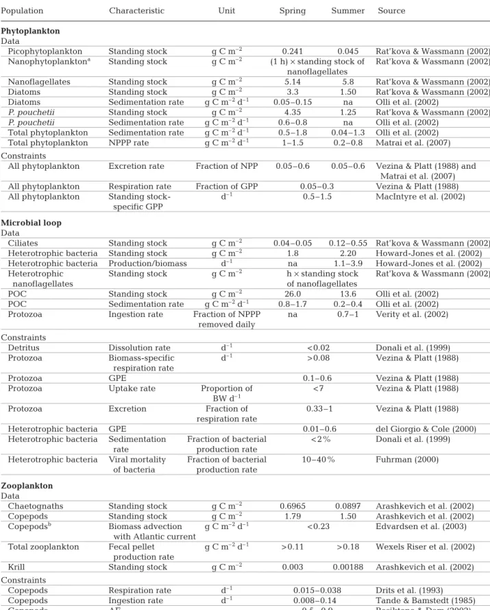
To benthos To DOC log(bactV: planktV) Recycling Protozoa 1.0 0.8 0.6 0.4 0.2 0.0 –0.2 –0.4

Fate of GPP Microbial loop COP diet

HF0 HF50 HF100 Microbial

Fig. 1. Differences between the 3 herbivorous food webs (grey: HF0, HF50 and HF100, from left to right, respectively) and the microbial food web (black). Left section — fate of gross primary production (GPP): proportions sinking to the benthos (To benthos) and excreted as dissolved organic car-bon (To DOC). Middle section — microbial loop: the logarithm of the ratio of bacterivory over planktivory by protozoa (log[bactV: planktV]; unitless), and the proportion of flows resulting from recycling (Recycling) as quantified by Finn’s cycling index. Right section — diet of copepods: proportion of protozoa in copepod diet (Protozoa). Bars represent 90% CI and were calculated by analysing all N realised solutions of

was lost by sinking in spring, while in summer this was only 5 to 10% (Fig 1). The percentage of GPP released as DOC was about 40% in spring and 50% in summer. In spring, release of DOC by phytoplankton repre-sented between 64 and 88% of all flows to the DOC compartment; in summer this was 41%. The remaining flows to DOC came from excretion by protozoa.

In the food web models, all DOC was taken up by bac-teria, which were subsequently grazed by protozoa. This bacterivory appeared at least as important as the phyto-plankton ingestion by protozoa because the pooled car-bon flows from bacteria to protozoa (heterotrophic nanoflagellates and ciliates) were in general 1.2 (spring) to 4 times (summer) higher than pooled carbon flows from the 3 phytoplankton groups to protozoa (Fig 1). For HF0, the protozoan diet was highly uncertain. Carbon recycling, as quantified by the FCI, was between 2 and 15% in spring, and reached 20% in summer.

During summer, the majority of the copepod diet (80 to 90%) consisted of protozoa while estimates for spring are less decisive and depend on the scenario chosen (20 to 80% heterotrophs in diet) (Fig 1).

Within the fish community, differences in food web flows between spring and summer could be largely attributed to the absence of capelin in the southern Barents Sea in summer. Adult cod that did not follow the capelin migrating north in summer (50% of the spring stock, see Material and methods), experienced a diet shift from capelin (spring) to krill (summer) (Table 2). The diet contribution of young cod and her-ring in adult cod was marginal. The diet of young cod always consisted of about 90% copepods (Table 2).

Dependency of cod on other food web compartments

In general, young cod were most dependent on copepods, their main food item (Fig. 2). In summer, the extended diet of young cod was dominated by ciliates, heterotrophic nanoflagellates, DOC and bacteria (hereafter termed ‘the microbial loop’), together with copepods. In spring, when the food web was herbivo-rous, the dependency of young cod was more equally distributed over other food web compartments. Each of the phytoplankton groups alone was of moderate importance for young cod with no apparent minima or maxima and, apart from pico- and nanoplankton, no between-month differences. The dependencies of adult cod were much more evenly distributed over all other food web compartments than for young cod, and seasonal differences were far less pronounced (Fig. 3). Adult cod were 3 times less dependent on the micro-bial loop than were young cod. In contrast, adult cod were 6 times more dependent on macrozooplankton (chaetognaths and krill) and 3 times more dependent

on planktivorous fish (capelin) than were young cod. Similar to our findings for young cod, differences between both months in dependencies on phytoplank-ton groups were not apparent for adult cod.

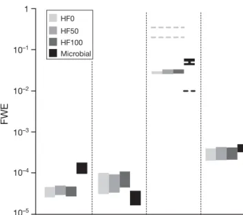
Food web efficiency

The FWE based on young cod production was between 2 × 10– 5_{and 5 × 10}– 5_{for spring and almost an}

order of magnitude higher in summer (Fig. 4). When Table 2. Diet of young and adult cod (three scenarios; % of

food intake ± 1 SD)

Krill Capelin Copepods Herring Young cod Spring HF0 4 ± 3 6 ± 4 89 ± 6 1 ± 1 Spring HF50 3 ± 2 5 ± 4 90 ± 7 2 ± 1 Spring HF100 4 ± 3 5 ± 4 90 ± 6 1 ± 1 Summer 2 ± 1 97 ± 2 1 ± 1 Adult cod Spring HF0 30 ± 6 54 ± 9 12 ± 3 4 ± 1 Spring HF50 31 ± 7 53 ± 11 12 ± 4 4 ± 1 Spring HF100 30 ± 6 55 ± 10 11 ± 3 4 ± 1 Summer 64 ± 2 28 ± 2 8 ± 1

Extended diet of young cod

Dependenc y DI A PHA AU T CO P CHA CI L HNA KRI DE T BAC DO C CAP CO D HER 0.0 0.2 0.4 0.6 0.8 1.0 1.2 1.4 HF0 HF50 HF100 Microbial --- --- --- --- --- --- --- --- --- --- --- ---

---Fig. 2. Proportions of the different food web compartments in the extended diet (‘dependency’, unitless) of young cod for 3 scenarios for spring (grey: HF0, HF50 and HF100) and for summer (black). Bars represent 90% CI and were calculated by analysing all N realisations per food web structure. DIA = diatoms, PHA = Phaeocystis pouchetii, AUT = autotrophic nanophytoplankton, COP = copepods, CHA = chaetognaths, CIL = ciliates, HNA = heterotrophic nanoflagellates, KRI = krill, DET = detrius, BAC = bacteria, DOC = dissolved organic

based on adult cod production, FWE was about 2 times higher in spring than in summer. When based on pro-duction of all fish (cod, capelin and herring), the food web was equally efficient in both seasons. The FWE based on with copepod production was 1.5 times higher in summer than in spring.

DISCUSSION DOC production

The estimates for DOC release by phytoplankton (in summer, up to 50% of GPP) are among the highest reported (Nagata 2000), but are consistent with most of the observations in other Arctic systems such as the Eastern North Water Polynya where Tremblay et al. (2006) found DOC release to be 30% (spring) and 50% (summer) of the net particulate production. Simi-lar values were also found for Antarctic oceans (Ander-son & Rivkin 2001). Modelling studies revealed rela-tively high DOC release by phytoplankton in temperate waters as well, e.g. 35% of the GPP in the northeastern Atlantic Ocean during spring (Fasham et al. 1999) and 65% of the photosynthetic carbon prod-ucts in estuary enclosures during a simulated bloom experiment (Van den Meersche et al. 2004). DOC release in the ice-covered Arctic is probably lower than in the ice-free regions discussed here, as sug-gested by data from the Chukchi Sea (Mathis et al.

2007) and from the West Antarctic Peninsula and the Ross Sea (Ducklow et al. 2006).

Processes resulting in phytoplankton DOC release in-clude incomplete digestion by grazers (Jumars et al. 1989), cell lysis by viruses and exudation (Anderson & Williams 1998). Inferring the importance of viral activity is not straightforward as quantitative infor-mation is scarce. A number of studies in the polar fresh-water environment exist (Anesio et al. 2007, Sawstrom et al. 2007), but information on the ice-free waters of the Barents Sea was not available. In the Chukchi Sea, another panarctic shelf sea, Hodges et al. (2005) showed that high bacterial and viral abundances coin-cided with algal blooms during summer. Hodges et al. (2005) also found that the bacterial community tends to converge towards less diverse, more specialist-dominated assemblages in summer, a process they at-tributed to viral activity. Clearly, the exact cause for high DOC release by phytoplankton certainly deserves more attention in future experimental work.

The importance of DOC excreted by heterotrophs, relative to the prime DOC source, i.e. release by phyto-plankton, is still under debate. Anderson & Williams (1998) considered the heterotrophic production to be negligible compared with DOC production by phyto-plankton for the English Channel, while others authors (Jumars et al. 1989, Strom et al. 1997) support the oppo-site view. Our results indicate that in spring, DOC

re-Dependenc y DI A PHA AU T CO P CHA CI L HNA KRI DE T BAC DO C

CAP YCO HER

0.0 0.2 0.4 0.6 0.8 1.0 1.2 1.4 HF0 HF50 HF100 Microbial ---

---Fig. 3. Proportions of the different food web compartments in the extended diet (‘dependency’, unitless) of adult cod for 3 scenarios for spring (grey: HF0, HF50 and HF100) and for summer (black). Bars represent 90% CI and were calculated

by analysing all N realisations per food web structure

FW E 1 10–1 10–2 10–3 10–4 10–5 HF0 HF50 HF100 Microbial --- ---

---YCO COD COP ALL FISH

Fig. 4. Food web efficiency (FWE, expressed as fraction) calculated by dividing the production of young cod (YCO), adult cod (COD), copepods (COP) and all fish (ALL FISH) by the sum of net primary production and input of copepod biomass by the Atlantic current. Dashed line: FWEs for cope-pod production found by Berglund et al. (2007). Bars repre-sent 90% CI and were calculated by analysing all N realised

lease by phytoplankton is the major source of DOC (> 50%). In summer, the opposite is true as 59% of flows to DOC come from protozoa and not from phytoplank-ton. These findings are in line with other modelling ex-ercises that show that DOC excretion by heterotrophs varies with season and is most important in summer when food webs are microbial (Fasham et al. 1999).

The microbial loop

The DOC produced by all processes was consumed by bacteria because it is the only sink of DOC. Such a tight control of the DOC stock by bacteria is realistic in marine ecosystems (Vargas et al. 2007) and in polar systems in particular. Evidence from experimental studies in the Bering Strait region and across to the Canadian Basin indicates that microbial production is primarily controlled by dissolved organic matter (DOM) availability rather than by physical forcing such as by temperature (Rich et al. 1997, Kirchman et al. 2005). Likewise, the distribution of heterotrophic bac-terial activity in the Kara Sea (Meon & Amon 2004) and Barents Sea (Thingstad et al. 2008) was controlled by the availability of DOC.

Bacterial production, essentially a reflection of DOC production because of the strong coupling discussed in the previous paragraph, was of comparable impor-tance as primary production to fulfill carbon require-ments of protozoa. In summer, protozoa fed 4 times more heavily on bacteria than on phytoplankton. This trend is amenable to other Arctic and Antarctic ecosys-tems. Becquevort et al. (2000) found that in the Indian sector of the Southern Ocean, protozoa principally ingested bacteria (87 to 99%) in both early spring and late summer. In summer, the diet of protozoa almost completely consisted of bacteria. Simek & Straskra-bova (1992) found bacterivory by protozoa in a reser-voir in Southern Bohemia to be negligible during spring, but protozoa consumed all bacterial production in summer. The same was found for the Canadian Arc-tic and McMurdo Sound in AntarcArc-tica (Anderson & Rivkin 2001).

An additional sink of DOC, not included in our model, might be photolysis of DOC. Photochemical mineralisation rates of terrestrial DOC have been found to exceed biological rates, although not for freshwater DOC (Obernosterer & Benner 2004). In the marine environment, photolysis is mostly considered as a transformation of aged refractory DOC to labile DOC (or directly to CO2) (Mopper et al. 1991).

Although we do not claim that photolysis of marine labile DOC is unimportant, this process is currently too poorly constrained for reliable incorporation in food web models (Kieber 2000). Additionally, the loss of

labile DOC by photolysis will to some extent be com-pensated by the creation of new labile DOC through photolysis of refractory DOC.

The dominance of bacteria over phytoplankton as a food source for protozoa, combined with the high protozoan excretion of DOC, which is again readily taken up by bacteria, enhanced recycling of carbon in summer as compared with spring. This recycling was quantified as the percentage of all flows that is gener-ated by recycling and is referred to as the Finn’s cycling index (FCI). FCI was between 2 and 15% in spring and covered the range reported for open oceanic systems (Heymans & Baird 2000). However, recycling in summer was nearly 20%, i.e. no longer in the range expected for open oceanic systems but rather representative of estuarine systems (Heymans & Baird 2000) rather than open oceanic systems. The role of protozoa in this carbon recycling is crucial, as can be seen from the very low FCI for HF0 (Fig. 1), i.e. the spring scenario where all nanoflagellates were assumed to be autotrophic. Although the HF0 scenario might be judged as unrealistic, given recent findings on mixotrophy (Zubkov & Tarran 2008), it appears to be a useful exercise that increases our insight into the role microbes play in marine systems.

Feeding on microbial carbon by copepods

Intensive feeding of copepods on protozoa is found in different marine ecosystems (Tamigneaux et al. 1997, Mayzaud et al. 2002, Calbet & Saiz 2005) although the intensity of this feeding process differs between systems. For example, the grazing of pods on protozoa was only half of the grazing of cope-pods on phytoplankton in all seasons and for different regions in the Greenland Sea (Moller et al. 2006). Car-mack & Wassmann (2006), as well as Levinsen et al. (2000) argued that feeding by copepods on protozoa especially occurs at low phytoplankton concentrations. In a recent cross-ecosystem analysis, Calbet & Saiz (2005) suggested a cut-off value for phytoplankton biomass (50 µg C l–1_{), below which ciliates contribute}

at least as much to the copepod diet as do phytoplank-ton. As Calbet & Saiz (2005) only considered ciliates as protozoa, this cut-off value may be higher when other protozoa such as heterotrophic nanoflagellates are included (as in the present study). The phytoplankton concentration in southern Barents Sea is about 50 µg C l–1_{in summer and 100 µg C l}–1_{in spring in the upper}

90 m of the water column (Rat’kova & Wassmann 2002). The fact that copepods feed on a mixture of autotrophs (20 to 80%) and protozoa in spring, while up to 90% of their diet consists of protozoa in summer, does agrees with the cross-ecosystem trends found by

Calbet & Saiz (2005). This seasonal diet shift typically coincides with a shift from large copepod species in spring to smaller species in summer that are perfectly suited for grazing on protozoa (Moller et al. 2006). This shift was experimentally confirmed by Arashkevich et al. (2002) for the southern Barents Sea.

Copepods: the link between the microbial loop and higher trophic levels

The diets we derived for adult and young cod, which corresponded well with independent stomach content data (Orlova et al. 2005, Link et al. 2009), have implica-tions for the ecological role of copepods. Copepods served as the main food item for young cod in both sea-sons. In summer, copepod production was closely linked to protozoa production, as shown by the propor-tion of protozoa in the copepod diet (Fig. 1). In turn, protozoa in summer relied heavily on bacteria that controlled the stock of DOC. Because of their interde-pendency, not only copepods, but also protozoa, bacte-ria and DOC were important for young cod in summer (Fig. 2). The dependencies of young cod indicated that > 60% of their diet passed through the microbial loop. As the fraction of heterotrophs in the copepod diet was lower in spring than in summer (Fig. 2), the depen-dency of young cod on the microbial loop was 2 to 3 times lower in spring than in summer. Instead, the dependencies on phytoplankton, protozoa, bacteria and DOC were comparable in spring. Still, the depen-dency on copepods was comparable for both food web structures indicating that copepods were always crucial for converting microbial carbon to forms con-sumable by cod. The unique coupling of the microbial domain with young cod through one important link (copepods), resulted in an interesting ‘hourglass’-like food web structure for young cod. The same hourglass-like structure was found for adult cod, albeit only in spring when the adult cod’s favourite food was capelin, a copepod feeder. This resulted in similar dependen-cies for young and adult cod in spring. In summer, the migration of capelin forced the adult cod population to feed on herbivorous krill, i.e. exclusively relying on phytoplankton and not on protozoa. This creates an uncoupling of adult cod from the microbial loop in summer, as reflected by the lower dependency for adult cod on the microbial loop than for young cod (Figs. 2 & 3).

Copepod biomass advection (0.03 g C m–2_d–1_{in both}

seasons) was 1.25 to 5 and 2.5 to 5 times lower than locally produced copepod biomass in spring and in summer, respectively. These differences could be expected from current measurements between Bear Island and the northern coast of Norway. Currents

were about 2 times higher in May 1998 than in July 1999 (Ingvaldsen et al. 2004), i.e. the months for which data were gathered (Table 1), and were in general high (≈2.5 Sverdrups [Sv]). One could thus expect that in years with lower net inflow rates, local phenomena become increasingly important, which would further strengthen the relationships between the microbial and fish communities established here.

Food web efficiency

The lower FWE for adult cod production in summer than in spring reflects the lower standing stock of cod during summer in the southern Barents Sea. Because of the lower resource requirements of this reduced cod stock, less carbon is transferred to cod in summer than in spring. Instead, carbon is transferred to the other fish compartments. As such, the food web cannot be said to be less efficient in summer, as can be seen from the FWE for production of all fish (Fig. 4). In contrast with adult cod, the reduction of the young cod stock in summer did not cause the FWE for young cod produc-tion to be lower in summer than in spring. Apparently, the higher efficiency of the carbon transfer from phyto-plankton to copepods in summer (Fig. 4), the main food for young cod in both seasons, compensated for the effect of a reduced young cod stock in summer.

The FWEs for fish production found here (Fig. 4) sug-gest a lower efficiency for fish production than the transfer efficiencies (TEs) assumed by Jennings et al. (2008) in their recent effort to estimate global fish pro-duction from primary propro-duction data. Using TE = FWE(TL – 1) –1_{as an approximation, our results indicate}

TEs of 0.05 to 0.13 for cod (with trophic level [TL] = 4.3 to 5.6), and of 0.01 to 0.11 for young cod (TL = 3.3 to 5), while Jennings et al. (2008) use a fixed TE of 0.125. Sensitivity analyses carried out by Jennings et al. (2008) demonstrated that the use of the TEs found here would lower their estimates of fish production by more than a factor of 2.

The FWE based on copepod production in summer was among the highest FWEs observed in an experi-mental microbial food web established by Berglund et al. (2007) (Fig. 4). However, the FWE for copepods in spring was 10 times lower than what Berglund et al. (2007) reported for an experimental herbivorous food web. For this apparent discrepancy between experi-mental data and our results, 2 explanations are offered. First, the use of mesocosms by Berglund et al. (2007) with 40 cm depth may have resulted in an underesti-mation of phytoplankton sedimentation, a loss term for the pelagic food web, and thus an overestimation of FWE. Second, the most abundant species in those mesocosms were of intermediate size (cryptophytes

and prasinophytes <10 µm) and were smaller than the phytoplankton that dominated the spring food webs discussed here (> 20 µm) (Rat’kova & Wassmann 2002). Phytoplankton in the enclosures described by Berglund et al. (2007) are thus intrinsically less prone to sedimentation than in the Barents Sea food webs described here. A recalculation of the FWE for copepods using the net primary production minus sedimentation losses (i.e. using NPP + ATL – SED as a denominator in Eq. (3) with SED representing the sedi-mentation losses) reveals that FWEs are comparable across the 4 food webs discussed in the present study (Fig. S3, Supplement 1). This indicates that the carbon remaining in the water column is processed as effi-ciently in the summer (microbial) food web than in the spring (herbivorous) food webs.

A contemporary view is that microbial food webs have more trophic levels and, thus, higher overall metabolic requirements (Straile 1997) when transferring carbon from the primary producers up to the top predators. However, in this paper we show that a higher number of trophic levels do not necessary result in lower FWEs for microbial food webs than for herbivorous food webs. Life forms that dominate in the microbial food web, i.e. bacteria and protozoa, essentially consume loss products from other food web compartments (e.g. excretion of DOC by protozoa and subsequent uptake by bacteria). As such, the fraction of the carbon fixed by phyto-plankton that reaches higher trophic levels would be higher than in herbivorous food webs, as suggested by Vargas et al. (2007) and Calbet & Saiz (2005).

As our estimates of DOC production, bacterivory by protozoa and consumption of protozoa by copepods were shown to reflect what is observed for many other food webs, our results may well extend beyond this particular case for the Barents Sea. However, the hetero-geneity of this system (Wassmann et al. 2006) would make extrapolation of our results to other regions or pe-riods within the Barents Sea speculative. For example, for periods with a collapsing capelin stock (Dalpadado & Bogstad 2004) in years with a strong link between ben-thic production and adult cod feeding, the trophic posi-tion of cod would likewise change and, thus, so would its dependencies. It would be interesting to determine how such spatiotemporal variability changes the conclusions drawn here, and we encourage future studies to examine such issues using the inverse modelling framework or other quantitative tools.

CONCLUSIONS

In spring (the herbivorous food web), release of DOC by phytoplankton dominated the carbon flows to the DOC compartment where it was consumed by

bacte-ria. Bacteria were of comparable importance as phyto-plankton as food for protozoa. The diet of copepods was a mixture of protozoa (20 to 80%) and phyto-plankton, which resulted in moderate dependency of young and adult cod on the microbial loop (DOC– bacteria–protozoa).

In summer (the microbial food web), protozoa excre-tion was more important than DOC release by phyto-plankton. Bacteria consuming this DOC were 4 times as important as a food source for protozoa as phyto-plankton. Protozoa in turn formed 80 to 90% of the copepod diet. Because of the strong relationships between the key players of the microbial loop (DOC, bacteria and protozoa) and copepods, the dependency of young cod on the microbial loop was high in sum-mer. Adult cod were far less dependent on the micro-bial loop than young cod as they relied on strictly herbivorous krill in summer.

The efficiency of the food web for fish compared well between seasons and for copepod production; FWE was 2 times higher in summer than in spring. For the summer case, FWE for copepod production agreed well with available data; for spring, our estimates were an order of magnitude lower than literature estimates from shallow enclosures with relatively small phyto-plankton species. Our estimates on DOC production, bacterivory by protozoa and consumption of protozoa by copepods agreed well with what has been observed for many other food webs (both polar and nonpolar), which suggests our results to be amenable to other parts of the world’s oceans.

Acknowledgements. This study was performed for the CORAMM (Coral Risk Assessment, Monitoring and Model-ling) project, which is funded by StatoilHydro. We thank A. Arashkevich, K. Olli and C. Wexels Riser for providing us with the raw data files of their sampling campaigns, and P. Wass-mann for a map of the study region. Three anonymous reviewers are gratefully acknowledged for their constructive feedback.

LITERATURE CITED

Ajiad AM, Pushchaeva TY (1992) The daily feeding dynamics in various length groups of the Barents Sea capelin. In: Bogstad B, Tjelmeland S (eds) Interrelations between fish populations in the Barents Sea. Proc 5th PINRO-IMR Symp, Murmansk, 1991. Institute of Marine Research, Bergen, p 181–192

Allesina S, Ulanowicz RE (2004) Cycling in ecological net-works: Finn’s index revisited. Comput Biol Chem 28: 227–233

Anderson MR, Rivkin RB (2001) Seasonal patterns in grazing mortality of bacterioplankton in polar oceans: a bipolar comparison. Aquat Microb Ecol 25:195–206

Anderson TR, Williams PJL (1998) Modelling the seasonal cycle of dissolved organic carbon at station E-1 in the Eng-lish Channel. Estuar Coast Shelf Sci 46:93–109

➤

➤

➤

➤

Anesio AM, Mindl B, Laybourn-Parry J, Hodson AJ, Sattler B (2007) Viral dynamics in cryoconite holes on a high Arctic glacier (Svalbard). J Geophys Res 112:G04S31 doi: 10.1029/2006JG000350.

Arashkevich E, Wassmann P, Pasternak A, Riser CW (2002) Seasonal and spatial changes in biomass, structure, and development progress of the zooplankton community in the Barents Sea. J Mar Syst 38:125–145

Arrhenius F (1998) Variable length of daily feeding period in bioenergetics modelling: a test with 0-group Baltic her-ring. J Fish Biol 52:855–860

Arrigo KR, Worthen D, Schnell A, Lizotte MP (1998) Primary production in Southern Ocean waters. J Geophys Res 103(C8):15587–15600

Azam F, Fenchel T, Field JG, Gray JS, Meyer-Reil LA, Thingstad F (1983) The ecological role of water-column microbes in the sea. Mar Ecol Prog Ser 10:257–263 Becquevort S, Menon P, Lancelot C (2000) Differences of the

protozoan biomass and grazing during spring and summer in the Indian sector of the Southern Ocean. Polar Biol 23: 309–320

Berglund J, Muren U, Bamstedt U, Andersson A (2007) Effi-ciency of a phytoplankton-based and a bacteria-based food web in a pelagic marine system. Limnol Oceanogr 52: 121–131

Besiktepe S, Dam HG (2002) Coupling of ingestion and defecation as a function of diet in the calanoid copepod Acartia tonsa. Mar Ecol Prog Ser 229:151–164

Bogstad B, Haug T, Mehl S (2000) Who eats whom in the Bar-ents Sea? NAMMCO Sci Publ 2:98–119

Calbet A, Saiz E (2005) The ciliate-copepod link in marine ecosystems. Aquat Microb Ecol 38:157–167

Carmack E, Wassmann P (2006) Food webs and physical– biological coupling on pan-Arctic shelves: unifying concepts and comprehensive perspectives. Prog Oceanogr 71:446–477

Cury PM, Shin YJ, Planque B, Durant JM and others (2008) Ecosystem oceanography for global change in fisheries. Trends Ecol Evol 23:338–346

Daan N (1975) Consumption and production in North Sea cod, Gadus morhua: an assessment of the ecological state of the stock. Neth J Sea Res 9:24–55

Dalpadado P, Bogstad B (2004) Diet of juvenile cod (age 0–2) in the Barents Sea in relation to food availability and cod growth. Polar Biol 27:140–154

Dalpadado P, Skjoldal HR (1996) Abundance, maturity and growth of the krill species Thysanoessa inermis and T. long-icaudata in the Barents Sea. Mar Ecol Prog Ser 144: 175–183 Davis J, Benner R (2007) Quantitative estimates of labile and semi-labile dissolved organic carbon in the western Arctic Ocean: a molecular approach. Limnol Oceanogr 52: 2434–2444

del Giorgio PA, Cole JJ (2000) Bacterial energetics and growth efficiency. In: Kirchman DL (ed) Microbial ecology of the oceans. Wiley, New York, p 289–325

Donali E, Olli K, Heiskanen AS, Andersen T (1999) Carbon flow patterns in the planktonic food web of the Gulf of Riga, the Baltic Sea: a reconstruction by the inverse method. J Mar Syst 23:251–268

Drits AV, Pasternak AF, Kosobokova KN (1993) Feeding, metabolism and body-composition of the Antarctic cope-pod Calanus propinquus Brady with special reference to its life cycle. Polar Biol 13:13–21

Ducklow HW, Fraser W, Karl DM, Quetin LB and others (2006) Water-column processes in the West Antarctic Peninsula and the Ross Sea: interannual variations and foodweb structure. Deep Sea Res II 53:834–852

Durant JM, Hjermann DO, Sabarros PS, Stenseth NC (2008) Northeast arctic cod population persistence in the Lofoten–Barents Sea system under fishing. Ecol Appl 18: 662–669

Edvardsen A, Tande KS, Slagstad D (2003) The importance of advection on production of Calanus finmarchicus in the Atlantic part of the Barents Sea. Sarsia 88:261–273 Falk-Petersen S, Hagen W, Kattner G, Clarke A, Sargent J

(2000) Lipids, trophic relationships, and biodiversity in Arctic and Antarctic krill. Can J Fish Aquat Sci 57: 178–191

Fasham M, Boyd P, Savidge G (1999) Modeling the relative contributions of autotrophs and heterotrophs to carbon flow at a Lagrangian JGOFS station in the Northeast At-lantic: the importance of DOC. Limnol Oceanogr 44: 80–94 Fuhrman J (2000) Impact of viruses on bacterial processes. In: Kirchman DL (ed) Microbial ecology of the oceans. Wiley, New York, p 327–350

Gasparovic B, Plavsic M, Boskovic N, Cosovic B, Reigstad M (2007) Organic matter characterization in Barents Sea and eastern Arctic Ocean during summer. Mar Chem 105: 151–165

Gjosaeter H, Dalpadado P, Hassel A, Skjoldal HR (2000) A comparison of performance of WP2 and MOCNESS. J Plankton Res 22:1901–1908

Hansson S, Rudstam LG, Kitchell JF, Hilden M, Johnson BL, Peppard PE (1996) Predation rates by North Sea cod (Gadus morhua): predictions from models on gastric evac-uation and bioenergetics. ICES J Mar Sci 53:107–114 Hendriks AJ (1999) Allometric scaling of rate, age and density

parameters in ecological models. Oikos 86:293–310 Heymans JJ, Baird D (2000) Network analysis of the northern

Benguela ecosystem by means of NETWRK and ECO-PATH. Ecol Model 131:97–119

Hjermann DO, Stenseth NC, Ottersen G (2004) The popula-tion dynamics of Northeast Arctic cod (Gadus morhua) through two decades: an analysis based on survey data. Can J Fish Aquat Sci 61:1747–1755

Hjermann DO, Bogstad B, Eikeset AM, Ottersen G, Gjosaeter H, Stenseth NC (2007) Food web dynamics affect North-east Arctic cod recruitment. Proc Biol Sci 274:661–669 Hodges LR, Bano N, Hollibaugh JT, Yager PL (2005)

Illustrat-ing the importance of particulate organic matter to pelagic microbial abundance and community structure—an Arctic case study. Aquat Microb Ecol 40:217–227

Holdway DA, Beamish FWH (1984) Specific growth rate and proximate body composition of Atlantic cod (Gadus morhua L). J Exp Mar Biol Ecol 81:147–170

Howard-Jones MH, Ballard VD, Allen AE, Frischer ME, Ver-ity PG (2002) Distribution of bacterial biomass and activVer-ity in the marginal ice zone of the central Barents Sea during summer. J Mar Syst 38:77–91

Huse G, Johansen GO, Bogstad B, Gjøsæter H (2004) Study-ing spatial and trophic interactions between capelin and cod using individual-based modelling. ICES J Mar Sci 61: 1201–1213

ICES (2005) Report of the northern pelagic and blue whiting fisheries working group (WGNPBW), 25 August –1 Sep-tember 2005. ICES Headquarters, Copenhagen

ICES (2008) Report of the Arctic fisheries working group (AFWG), 21–29 April 2008. ICES Headquarters, Copen-hagen

Ingvaldsen RB, Asplin L, Loeng H (2004) The seasonal cycle in the Atlantic transport to the Barents Sea during the years 1997–2001. Cont Shelf Res 24:1015–1032

Jennings S, Melin F, Blanchard JL, Forster RM, Dulvy NK, Wilson RW (2008) Global-scale predictions of community

➤

➤

➤

➤

➤

➤

➤

➤

➤

➤

➤

➤

➤

➤

➤

➤

➤

➤

➤

➤

➤

➤

➤

➤

➤

➤

➤

➤

➤

➤

➤

➤

➤

➤

and ecosystem properties from simple ecological theory. Proc Biol Sci 275:1375–1383

Jumars PA, Penry DL, Baross JA, Perry MJ, Frost BW (1989) Closing the microbial loop: dissolved carbon pathway to heterotrophic bacteria from incomplete ingestion, diges-tion and absorpdiges-tion in animals. Deep Sea Res Part A 36: 483–495

Karamushko LI, Christiansen JS (2002) Aerobic scaling and resting metabolism in oviferous and post-spawning Bar-ents Sea capelin Mallotus villosus villosus (Muller, 1776). J Exp Mar Biol Ecol 269:1–8

Kieber DJ (2000) Photochemical production of biological sub-strates. In: de Mora SJ, Demers SJS, Vernet M (eds) The effects of UV radiation in the marine environment. Cam-bridge University Press, New York, p 130–148

Kirchman DL, Malmstrom RR, Cottrell MT (2005) Control of bacterial growth by temperature and organic matter in the Western Arctic. Deep Sea Res II 52:3386–3395

Klepper O, Vandekamer JPG (1987) The use of mass balances to test and improve the estimates of carbon fluxes in an ecosystem. Math Biosci 85:37–49

Klumpp DW, Vonwesternhagen H (1986) Nitrogen balance in marine fish larvae: influence of developmental stage and prey density. Mar Biol 93:189–199

Kones JK, Soetaert K, van Oevelen D, Owino JO (2009) Are network indices robust indicators of food web functioning? A Monte Carlo approach. Ecol Model 220:370–382 Legendre L, Rassoulzadegan F (1995) Plankton and nutrient

dynamics in marine waters. Ophelia 41:153–172

Levinsen H, Turner JT, Nielsen TG, Hansen BW (2000) On the trophic coupling between protists and copepods in arctic marine ecosystems. Mar Ecol Prog Ser 204:65–77 Link JS, Bogstad B, Sparholt H, Lilly GR (2009) Trophic role of

Atlantic cod in the ecosystem. Fish Fish 10:58–87 MacIntyre HL, Kana TM, Anning T, Geider RJ (2002)

Photoacclimation of photosynthesis irradiance response curves and photosynthetic pigments in microalgae and cyanobacteria. J Phycol 38:17–38

Mathis JT, Hansell DA, Kadko D, Bates NR, Cooper LW (2007) Determining net dissolved organic carbon production in the hydrographically complex western Arctic Ocean. Lim-nol Oceanogr 52:1789–1799

Matrai P, Vernet M, Wassmann P (2007) Relating temporal and spatial patterns of DMSP in the Barents Sea to phyto-plankton biomass and productivity. J Mar Syst 67:83–101 Mayzaud P, Tirelli V, Errhif A, Labat JP, Razouls S, Perissinotto R (2002) Carbon intake by zooplankton. Importance and role of zooplankton grazing in the Indian sector of the Southern Ocean. Deep Sea Res II 49: 3169–3187

Megrey BA, Rose KA, Klumb RA, Hay DE, Werner FE, Eslinger DL, Smith SL (2007) A bioenergetlics-based population dynamics model of Pacific herring (Clupea harengus pallasi) coupled to a lower trophic level nutrient –phytoplankton–zooplankton model: description, calibration, and sensitivity analysis. Ecol Model 202: 144–164

Mehl S (1989) The Northeast Arctic cod stock’s consumption of commercially exploited prey species in 1984–1986. Rapp P-V Reun 188:185–205

Meon B, Amon RMW (2004) Heterotrophic bacterial activity and fluxes of dissolved free amino acids and glucose in the Arctic rivers Ob, Yenisei and the adjacent Kara Sea. Aquat Microb Ecol 37:121–135

Moller EF, Nielsen TG, Richardson K (2006) The zooplankton community in the Greenland Sea: composition and role in carbon turnover. Deep Sea Res I 53:76–93

Mopper K, Zhou XL, Kieber RJ, Kieber DJ, Sikorski RJ, Jones RD (1991) Photochemical degradation of dissolved organic carbon and its impact on the oceanic carbon cycle. Nature 353:60–62

Nagata T (2000) Production mechanisms of dissolved organic matter. In: Kirchman DL (ed) Microbial ecology of the oceans. Wiley, New York, p 121–152

Obernosterer I, Benner R (2004) Competition between bio-logical and photochemical processes in the mineraliza-tion of dissolved organic carbon. Limnol Oceanogr 49: 117–124

Ogawa H, Amagai Y, Koike I, Kaiser K, Benner R (2001) Pro-duction of refractory dissolved organic matter by bacteria. Science 292:917–920

Olli K, Riser CW, Wassmann P, Ratkova T, Arashkevich E, Pasternak A (2002) Seasonal variation in vertical flux of biogenic matter in the marginal ice zone and the central Barents Sea. J Mar Syst 38:189–204

Orlova EL, Dolgov AV, Rudneva GB, Nesterova VN (2005) The effect of abiotic and biotic factors on the importance of macroplankton in the diet of Northeast Arctic cod in recent years. ICES J Mar Sci 62:1463–1474

Pauly D, Christensen V, Walters C (2000) Ecopath, Ecosim, and Ecospace as tools for evaluating ecosystem impact of fisheries. ICES J Mar Sci 57:697–706

Pedersen T, Nilsen M, Nilssen EM, Berg E, Reigstad M (2008) Trophic model of a lightly exploited cod-dominated ecosystem. Ecol Model 214:95–111

Pogson GH, Fevolden SE (1998) DNA heterozygosity and growth rate in the Atlantic cod Gadus morhua (L). Evolu-tion 52:915–920

R Development Core Team (2009) R: a language and environ-ment for statistical computing. R Foundation for Statistical Computing, Vienna

Rand PS, Stewart DJ (1998) Prey fish exploitation, salmonine production, and pelagic food web efficiency in Lake Ontario. Can J Fish Aquat Sci 55:318–327

Rat’kova TN, Wassmann P (2002) Seasonal variation and spa-tial distribution of phyto- and protozooplankton in the cen-tral Barents Sea. J Mar Syst 38:47–75

Reeve MR, Cosper TC (1975) Chaetognatha. In: Giese AC, Pearse JS (eds) Reproduction of marine invertebrates. II. Entoprocts and lesser coelomates. Academic Press, New York, p 157–184

Rich J, Gosselin M, Sherr E, Sherr B, Kirchman DL (1997) High bacterial production, uptake and concentrations of dissolved organic matter in the Central Arctic Ocean. Deep Sea Res II 44:1645–1663

Ross RM, Hofmann EE, Quetin LB (1996) Foundations for eco-logical research west of the Antarctic Peninsula. AGU Antarct Res Ser Am Geophys Union, Washington, DC Rudstam LG, Lindem T, Hansson S (1988) Density and in situ

target strength of herring and sprat: a comparison between 2 methods of analyzing single-beam sonar data. Fish Res 6:305–315

Sabine CL, Feely RA, Gruber N, Key RM and others (2004) The oceanic sink for anthropogenic CO2. Science 305:367–371

Sakshaug E, Bjorge A, Gulliksen B, Loeng H, Mehlum F (1994) Structure, biomass distribution, and energetics of the pelagic ecosystem in the Barents Sea: a synopsis. Polar Biol 14:405–411

Sawstrom C, Laybourn-Parry J, Graneli W, Anesio AM (2007) Heterotrophic bacterial and viral dynamics in Arctic freshwaters: results from a field study and nutrient-temperature manipulation experiments. Polar Biol 30: 1407–1415

➤

➤

➤

➤

➤

➤

➤

➤

➤

➤

➤

➤

➤

➤

➤

➤

➤

➤

➤

➤

➤

➤

➤

➤

➤

➤

➤

➤