Vibrations of a beam with a unilateral spring. Periodic solutions - Nonlinear normal modes

(1)

HAL Id: tel-00520999

https://tel.archives-ouvertes.fr/tel-00520999

Submitted on 24 Sep 2010

HAL is a multi-disciplinary open access

archive for the deposit and dissemination of sci-entific research documents, whether they are pub-lished or not. The documents may come from teaching and research institutions in France or abroad, or from public or private research centers.

L’archive ouverte pluridisciplinaire HAL, est destinée au dépôt et à la diffusion de documents scientifiques de niveau recherche, publiés ou non, émanant des établissements d’enseignement et de recherche français ou étrangers, des laboratoires publics ou privés.

Vibrations of a beam with a unilateral spring. Periodic

solutions - Nonlinear normal modes

H. Hazim

To cite this version:

H. Hazim. Vibrations of a beam with a unilateral spring. Periodic solutions - Nonlinear normal modes. Mathematics [math]. Université Nice Sophia Antipolis, 2010. English. �tel-00520999�

(2)

UNIVERSITÉ DE NICE-SOPHIA ANTIPOLIS - UFR Sciences

École Doctorale Sciences Fondamentales et Appliquées

THÈSE

Pour obtenir le titre de

Docteur en Sciences

de l’UNIVERSITÉ de Nice-Sophia Antipolis

Spécialité : MATHÉMATIQUES

présentée et soutenue par

Hamad Hazim

Vibrations of a beam with a unilateral spring.

Periodic solutions - Nonlinear normal modes

Thèse dirigée par Bernard Rousselet Soutenue le 05 Juillet 2010

M. Hedy Attouch Professeur, Université de Montpellier II Rapporteur M. Yann Brenier Directeur de recherche, UNSA Examinateur M. Neil Ferguson Senior Lecturer, University of Southampton, U.K. Examinateur M. Alain Léger Directeur de recherche, L.M.A. CNRS, Marseille Rapporteur Mme. Francesca Rapetti Maître de Conférence, HdR, UNSA Examinateur

M. Bernard Rousselet Professeur, UNSA Directeur

M. Jérôme Buffe Responsable Ingénierie Mécanique, Thales Alenia Space Invité

Laboratoire J.-A.Dieudonné Université de Nice

(3)

(4)

(5)

(6)

Remerciements

Je voudrais, en premier lieu, remercier mon directeur de thèse, Bernard Rousselet, Pro-fesseur à l’UNSA, pour ce qu’il m’a apporté durant ces trois années, mais aussi pour sa patience, pour le temps qu’il m’a consacré et évidemment pour son bon encadrement lors de la thèse.

Je tiens à remercier Professeur Alain Léger, pour le temps qu’il a consacré à la lecture de ce mémoire et à la rédaction du rapport. Je le remercie également pour ses commentaires con-structifs et ses suggestions, en particulier durant les journées du GDR 2501 d’acoustique. Merci également au Professeur Hedy Attouch pour avoir accepter de rapporter sur cette thèse, pour ses suggestions et pour sa présence au sein du jury.

Je souhaite également remercier les examinateurs, M.Yann Brenier, directeur de recherche à l’UNSA, M. Neil Ferguson, senior lecturer at the University of Southampton, M. Jérome Buffe, responsable ingénierie Mécanique à Thales Alenia Space et Mme Francesca Rapetti, Maître de conférence et HdR à l’UNSA, pour avoir accepté d’être présents aujourd’hui. Je remercie la direction de la société Thales Alenia Space, France, pour le financement de cette thèse. En espérant que le travail présenté soit au niveau de leur attente. Je ne peux pas passer sur cet aspect sans citer les efforts de mon directeur et de Mme Samia Gill pour établir ce contrat de recherche.

Je remercie aussi Mme Stéphanie Behar, responsable Cellule Expertise Mécanique et M. Jérôme Buffe qui ont suivi la thèse du côté de Thales Alenia Space. Ce travail n’aurait pas été accompli de cette façon sans leur support, notamment sur la partie expérimentale. Je tiens également à remercier M. Grégory Ladurrée qui s’occupait de cette thèse avant son départ pour l’ESA.

Mes remerciements vont aussi à M. Gérard Vanderborck, M.Bernard Grangier, M. Marc Constancio et M.Roger Thannberger de Thales Underwater System, Sophia Antipolis, pour leur aide et pour le bon déroulement des essais expérimentaux.

Je remercie M. Stéphane Junca, Maître de conférence à l’UNSA, avec lequel j’ai eu la chance de travailler et de discuter surtout sur la partie analytique.

Je suis reconnaissant au Professeur Gérard Iooss pour ses conseils, ses explications et sa disponibilité.

(7)

Je suis aussi reconnaissant à M. Abdul Habbal, Maître de conférence à l’UNSA, qui m’a profondément soutenu durant la préparation de cette thèse, et à M. Mohammad El Kadi, Maître de conférence à l’UNSA, qui m’a beaucoup aidé sur différents aspects, notamment au début lors de mon arrivé au laboratoire.

J’exprime ma gratitude envers tout les membres du laboratoire Jean Alexandre Dieudonné, Professeurs, Maîtres de conférence, Ingénieurs, personnes administratives et techniciens, pour m’avoir accueilli durant ces trois ans. Je remercie les responsables de l’école doctor-ale EDSFA et du CED pour le bon suivi des doctorants ainsi que pour toutes les formations proposées.

I gratefully thank Doctor Neil Ferguson and all members of the Institute of Sound and Vibra-tions Research, Southampton, U.K., where I spent around two months. This period was very important for the success of the experimental part of the thesis.

Je tiens à remercier mes professeurs de l‘université libanaise à Tripoli où j’ai eu mon pre-mier diplôme en mathématiques.

Durant ces trois ans, j’ai eu la chance de rencontrer plusieurs amis avec lesquel j’ai partagé des bons moments. Notamment (Sans ordre :-) ) Sarrage (10 ans?!), Hanzoul (habibi), Hayssam (ahla 3alam), Akhi Osman (Tibe.. :-)), Ahed (Rafik), Soleiman (3ala rassi), Jérôme (sympa co-bureau essa-essa-essatement), Thang (co-bureau très force! magnifisse!), Luca (amico!), Nikolas (amigo!), Sami, Federicco (il mio caz.. maestro d’italiano :-)), Nahla, Houssam (l’Ingénieur l khadoum), Taleb, Claire (pré-rapporteur de tout :)), Nadia, Isabelle (mach 3 en fr) et Wassila (atyab couscous :-)). Je n’oublie pas les collègues doctorants et ancien doctorants du laboratoire J.A.D que j’ai eu l’honneur de les connaitre.

Je suis reconnaissant à mon oncle Ali Assaad et sa famille qui m’ont accueilliet m’ont soutenu surtout au début de mon arrivée en France, merci!

A propos de Cristina, c’est une amie exceptionnelle que j’ai eu la chance de la connaitre. Elle était toujours et continue à être à mon coté. Je te remercie pour tout le bien que tu m’as apporté (Ch, Laz, am1, am2, ma, lat etc... :-)). Ti auguro tutti le fortune nel tuoi progetti! Mes “11” soeurs et frères étaient mon support solide depuis toujours, notamment Fida et Oussama, avec lesquels j’ai vécu la période la plus difficile au Liban, grazie! Ca ne sera pas complet si je ne cite pas (dans l’ordre décroissant :)) Louàa, Samar, Inad, Abed, Racha, Bassel, Malak, Asraa, Sara et ma nièce Nathalia et bien sure son père Mouamar.

Finalement, cette thèse est dédiée aux personnes qui la méritent, ma mère et mon père! C’est un petit cadeau négligeable devant la vie qu’ils ont sacrifié pour élever cette grande famille.

(8)

(9)

(10)

ex-pansions . . . 128 4.4.6 Nonlinear normal mode of a beam with a unilateral spring . . . 132 4.5 Nonlinear normal modes and forced systems . . . 135 4.5.1 Multiple scales expansion of forced system with unilateral contact . 135 4.5.2 Bounds on the remainder . . . 137 4.5.3 Approximate steady state solution . . . 141 4.5.4 Stability of the approximate solution . . . 142 4.5.5 Alternative Calculation of the nonlinear normal modes with an

exci-tation force . . . 142 4.5.6 Numerical results of a cantilever beam with a unilateral elastic contact 144 4.6 conclusion . . . 147

List of Figures

1.1 Beam system in unilateral contact with a bumper modeled as a linear spring. 25 1.2 Schematic of the cantilever Beam and the unilateral contact, the snubber was

modelled as a linear spring. . . 28 1.3 Photo of the cantilever aluminum beam on a shaker with four accelerometers. 29 1.4 The cantilever aluminum beam in contact with the Solithane snubber at the

free end. The whole system is based on a shaker which produces a harmonic motion of support given as an imposed acceleration a(s) = −a

ω2d(s). . . . . 29

1.5 The frequency contents of the measured (dashed line) and the predicted (solid line) acceleration for an excitation at 45 Hz and for a magnitude of 2g. The data are measured above the elastic support, the frequency axis is normalized by the excitation frequency. . . 35 1.6 The frequency contents of the measured (dashed line) and the predicted (solid

line) acceleration for an excitation at 65 Hz and for a magnitude of 2g. The data are measured above the elastic support, the frequency axis is normalized by the excitation frequency. . . 36 1.7 The frequency contents of the measured (dashed line) and the predicted (solid

line) acceleration for an excitation at 78 Hz and for a magnitude of 2g. The data are measured above the elastic support, the frequency axis is normalized by the excitation frequency. . . 36

(13)

1.8 The frequency contents of the measured (dashed line) and the predicted (solid line) acceleration for an excitation at 160 Hz and for a magnitude of 2g. The data are measured above the elastic support, the frequency axis is normalized by the excitation frequency. . . 37 1.9 the predicted (a) and the measured (b) acceleration for an excitation at 45 Hz

and for a magnitude of 2g; the data are measured above the elastic support . 37 1.10 the predicted (a) and the measured (b) acceleration for an excitation at 65 Hz

and for a magnitude of 2g; the data are measured above the elastic support . 37 1.11 the predicted (a) and the measured (b) acceleration for an excitation at 78 Hz

and for a magnitude of 2g; the data are measured above the elastic support . 38 1.12 the predicted (a) and the measured (b) acceleration for an excitation at 160

Hz for a magnitude of 2g; the data are measured above the elastic support . 38 1.13 The numerical displacement of the free end of the beam for an excitation at

45 Hz and 65 Hz, the magnitude of excitation is 2g. . . . 38 1.14 The numerical displacement of the free end of the beam for an excitation at

78 Hz and 160 Hz, the magnitude of excitation is 2g . . . . 39 1.15 The predicted force time signal for an excitation at 45 Hz and 65 Hz, the

magnitude of excitation is 2g. The force is induced by the spring contact. . . 39 1.16 The predicted force time signal for an excitation at 78 Hz and 160 Hz, the

magnitude of excitation is 2g. The force is induced by the spring contact. . . 40 1.17 Frequency sweep of the system with unilateral contact (solid line) compared

to the sweep of the cantilever beam without contact (dashed line). The first natural frequency of the linear system is shifted to the right to become the first nonlinear frequency. The harmonics of this nonlinear frequency also appear as well as the subharmonics of the second nonlinear frequency. . . . 40 1.18 Frequency sweep around the position of the first linear normal mode and the

corresponding nonlinear normal modes with its harmonics. . . 41 1.19 The frequency contents of the measured (dashed line) and the predicted (solid

line) acceleration for an excitation at 465 Hz and for a magnitude of 1g. The data is measured above the elastic support, the frequency axis is normalized by the excitation frequency. The response contains a single peak which mean that the system responds linearly. . . 43 1.20 The input imposed acceleration frequency contents measured on the shaker

for an excitation at 465 Hz and a magnitude of 1g, it is not a single sine wave excitation as there is some noise. The small peaks appears also in the response corresponding to this excitation. . . 44 1.21 The frequency contents of the measured (dashed line) and the predicted (solid

line) acceleration for an excitation at 90 Hz and for a magnitude of 0.5g. The data is measured above the elastic support, the frequency axis is normalized by the excitation frequency. The response contains a single peak which mean that the system responds linearly. . . 44 1.22 The input imposed acceleration frequency contents measured on the shaker

for an excitation at 90 Hz and a magnitude of 0.5g, it is not a single sine wave excitation as there is some noise. The small peaks appears also in the response corresponding to this excitation. . . 45

(14)

1.23 The frequency contents of the measured (dashed line) and the predicted (solid line) acceleration for an excitation at 160 Hz and for a magnitude of 5g. The data is measured above the elastic support, the frequency axis is normalized by the excitation frequency. The response contains all the harmonics which means that the system responds nonlinearly. . . 45 1.24 The frequency contents of the measured (dashed line) and the predicted (solid

line) acceleration for an excitation at 90 Hz and for a magnitude of 3g. The data is measured above the elastic support, the frequency axis is normalized by the excitation frequency. The response contains all the harmonics which means that the system responds nonlinearly. . . 46 1.25 The frequency contents of the measured (dashed line) and the predicted (solid

line) acceleration for an excitation at 220 Hz and for a magnitude of 8g. The data is measured above the elastic support, the frequency axis is normalized by the excitation frequency. The response contains all the harmonics which means that the system responds nonlinearly. . . 46 1.26 The frequency contents of the measured (dashed line) and the predicted (solid

line) acceleration for an excitation at 465 Hz and for a magnitude of 15g. The data is measured above the elastic support, the frequency axis is normalized by the excitation frequency. The response contains all the harmonics which means that the system responds nonlinearly. . . 47 1.27 The numerical displacement of the free end of the beam for an excitation at

90 Hz, the magnitude of excitation is 0.5g. The signal corresponds to a linear system with a positive mean. . . 47 1.28 The numerical displacement of the free end of the beam for an excitation at

465 Hz, the magnitude of excitation is 1g. The signal corresponds to a linear system with a positive mean. . . 48 1.29 The numerical displacement of the free end of the beam for an excitation

at 45 Hz, the magnitude of excitation is 3g. The signal corresponds to a nonlinear system with a positive mean. . . 48 1.30 The numerical displacement of the free end of the beam for an excitation

at 90 Hz, the magnitude of excitation is 3g. The signal corresponds to a nonlinear system with a positive mean. . . 49 1.31 The numerical displacement of the free end of the beam for an excitation

at 160 Hz, the magnitude of excitation is 5g. The signal corresponds to a nonlinear system with a positive mean. . . 49 1.32 The predicted force time signal for an excitation at 90 Hz, the magnitude

of excitation is 0.5g. The force is induced by the spring contact, it is linear with the same period as the corresponding acceleration and it is permanently positive. . . 50 1.33 The predicted force time signal for an excitation at 465 Hz, the magnitude

of excitation is 1g. The force is induced by the spring contact, it is linear with the same period as the corresponding acceleration and it is permanently positive. . . 50

(15)

1.34 The predicted force time signal for an excitation at 45 Hz, the magnitude of excitation is 3g. The force is induced by the spring contact, it is nonlinear with the same period as the corresponding acceleration and it is permanently positive. . . 51 1.35 The predicted force time signal for an excitation at 90 Hz, the magnitude of

excitation is 3g. The force is induced by the spring contact, it is nonlinear with the same period as the corresponding acceleration and it is permanently positive. . . 51 1.36 The predicted force time signal for an excitation at 465 Hz, the magnitude of

excitation is 15g. The force is induced by the spring contact, it is nonlinear with the same period as the corresponding acceleration and it is permanently positive. . . 52 1.37 The frequency contents of the measured (dashed line) and the predicted (solid

line) acceleration for an excitation at 45 Hz and for a magnitude of 2g for 5mm of backlash. The data is measured above the elastic support, the fre-quency axis is normalized by the excitation frefre-quency. The response contains all the harmonics which means that the system responds nonlinearly. . . 54 1.38 The frequency contents of the measured (dashed line) and the predicted (solid

line) acceleration for an excitation at 65 Hz and for a magnitude of 3g for 5mm of backlash. The data is measured above the elastic support, the fre-quency axis is normalized by the excitation frefre-quency. The response contains all the harmonics which means that the system responds nonlinearly. . . 54 1.39 The frequency contents of the measured (dashed line) and the predicted (solid

line) acceleration for an excitation at 110 Hz and for a magnitude of 13g for 5mm of backlash. The data is measured above the elastic support, the fre-quency axis is normalized by the excitation frefre-quency. The response contains all the harmonics which means that the system responds nonlinearly. . . 55 1.40 The numerical displacement of the free end of the beam for an excitation

at 65 Hz, the magnitude of excitation is 3g. The signal corresponds to a nonlinear system. . . 55 1.41 The numerical displacement of the free end of the beam for an excitation

at 110 Hz, the magnitude of excitation is 13g. The signal corresponds to a nonlinear system. . . 56 1.42 The predicted force time signal for an excitation at 65 Hz, the magnitude of

excitation is 3g. The force is induced by the spring contact. . . . 56 1.43 The predicted force time signal for an excitation at 110 Hz, the magnitude of

excitation is 13g. The force is induced by the spring contact. . . . 57 1.44 Frequency sweep of the system with unilateral spring in a backlash position

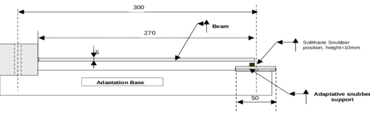
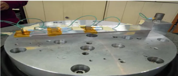
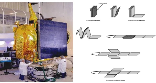
(solid line) compared to the sweep of the linear free beam (dashed line). Both curves overlay at the frequency where the beam looses contact with the spring. This frequency point depends on the excitation magnitude. . . 57 2.1 A schematic of the experimental setup. . . 63 2.2 Left: Solar array of a satellite under a test on a shaker. Right: A solar array from the

(16)

2.3 beam system with an unilateral spring under a periodic excitation . . . 69 2.4 The rig used for the experiments: a linear clamped-free beam in contact with a

rubber support (enlarged photograph on the right). . . 70 2.5 Predicted (solid) and measured displacements (dashed) (dB) for an excitation

at 32 Hz applied to the beam with unilateral support stiffness. The displace-ment is normalized by the peak value and is measured immediately above the support and the frequency axis is normalized by the excitation frequency. 70 2.6 Predicted (solid) and measured displacements (dashed) (dB) for an excitation

at 124 Hz applied to the beam with unilateral support stiffness. The displace-ment is normalized by the peak value and is measured immediately above the support and the frequency axis is normalized by the excitation frequency. 71 2.7 Predicted (solid) and measured displacements (dashed) (dB) for an excitation

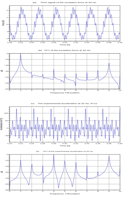
at 100 Hz applied to the beam with unilateral support stiffness. The displace-ment is normalized by the peak value and is measured immediately above the support and the frequency axis is normalized by the excitation frequency. 71 2.8 Measured excitation force (a) and its frequency contents (b), measured

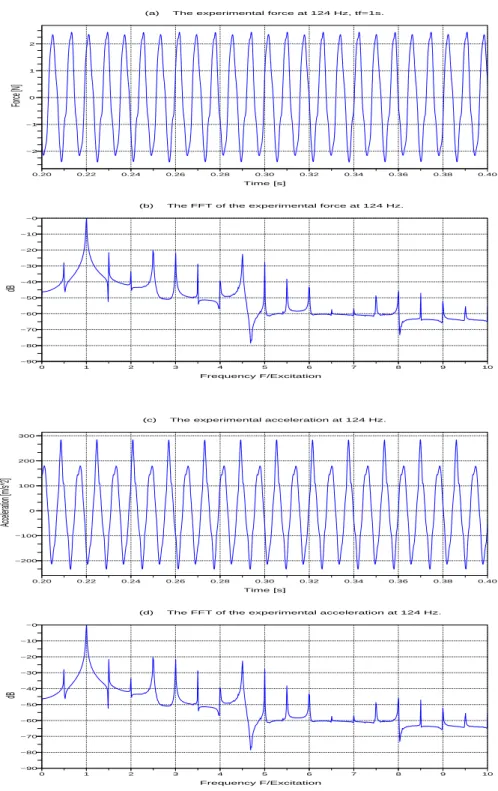
ac-celeration response (c) and its frequency content (d) for an excitation at 32 Hz. Strictly the force is not harmonic. . . 72 2.9 Measured excitation force (a) and its frequency contents (b), the measured

acceleration response (c) and its frequency content (d) for an excitation at 124 Hz. Strictly the force is not harmonic. . . 73 2.10 The predicted displacements for an excitation at 32 Hz; the displacement is

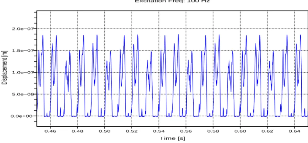
measured immediately above the support. The high unilateral stiffness yields almost a positive displacement. . . 74 2.11 The predicted displacements for an excitation at 124 Hz, the displacement is

measured immediately above the support. . . 74 2.12 The predicted displacements for an excitation at 100 Hz, the displacement is

measured immediately above the support. . . 75 2.13 The normalized mean square responses (mean square displacement divided

by the mean square excitation force) in each harmonic for inputs at three different mean square force levels. The excitation frequency is 32 Hz, the acceleration is measured immediately above the support. . . 75 2.14 The predicted displacements for a sine excitation at 32 Hz, The acceleration

magnitude is a = 1 m/s2_{. The displacement is measured immediately above} the support. . . 76 2.15 The predicted displacements for a sine excitation at 124 Hz. The acceleration

magnitude is a = 1 m/s2_{. The displacement is measured immediately above} the support. . . 76 2.16 The frequency content of the predicted numerical displacement for sine

exci-tation at 32 Hz, the displacement is measured immediately above the support. The excitation frequency is split into all its harmonics. . . 77 2.17 The predicted elastic force of the spring support for an excitation at 32 Hz.

The acceleration magnitude is a = 0.1m/s2_{and the spring is only in contact} at times where the beam displacement is negative. . . 77

(17)

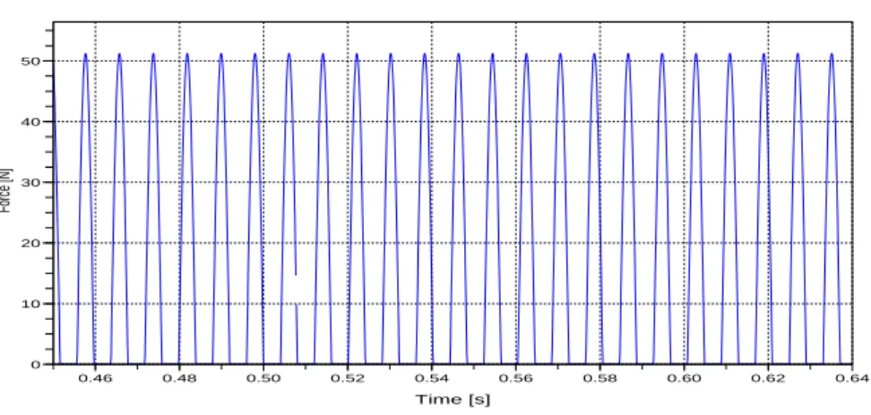
2.18 The predicted elastic force of the spring support for an excitation at 124 Hz. The acceleration magnitude is a = 0.1m/s2_{and the spring is only in contact} at times where the beam displacement is negative. . . 78 2.19 beam system with an unilateral spring under a periodic excitation . . . 78 2.20 Predicted (solid) and measured displacements (dB) for an excitation at 122

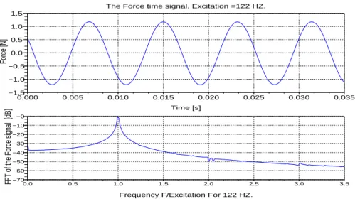
Hz applied to the beam with unilateral support stiffness. The displacement is measured immediately above the support and the frequency axis is normal-ized by the excitation frequency. . . 79 2.21 The time signal and its FFT of the input force for an excitation at 122 Hz. . 80 2.22 Predicted (solid) and measured displacements (dB) for an excitation at 32

Hz applied to the beam with unilateral support stiffness. The displacement is measured immediately above the support and the frequency axis is normal-ized by the excitation frequency. . . 81 3.1 A mass-spring model with a cubic component. . . 95 3.2 The displacements of the six nodes for the fourth nonlinear normal mode,

the period is Tn2 = 3.93 s and the corresponding frequency is fn2 = 0.254

Hz. All the components have the same period and they reach their maximum at the same time. 66 steps in ² to reach this nonlinearity, The value of the functional J²at the last iteration is 10(−6)and the average CPU time is 0.06 s

for a calculation of the function and the gradient. The total CPU time is 6.6 minutes. . . 97 3.3 The displacements of the fifth node (a) and the first node (b) of the linear

system (dashed line) and of the nonlinear system (solid line) for the second nonlinear normal mode. . . 97 3.4 The displacements of all nodes as function of the fifth one, the curves are not

straight lines and their shapes depend on the form of the nonlinearity. . . 98 3.5 The second nonlinear frequency of the system as function of the

nonlinear-ity (a), the FFT of the displacement for an integration time of 50 nonlinear period (b). . . 98 3.6 The phase space (solid line) compared to the corresponding linear phase

space (dashed line) of the fifth node (a) and the fourth node (b). . . 99 3.7 A mass-spring model with a unilateral component. . . 99 3.8 The displacements of the six nodes for the fourth nonlinear normal mode,

the period is Tn2 = 4.011 s and the corresponding frequency is fn2 = 0.249

Hz. All the components have the same period and they reach their maximum at the same time. 35 steps in ² to reach this nonlinearity, The value of the functional J² at the last iteration is 10(−6) and the average CPU time is 0.08

s for a calculation of the functional and the gradient, the total CPU time of optimization is 4.65 minutes. . . 100 3.9 The configuration and the phase spaces for the fourth nonlinear normal mode

for ² = 0.5. The lines in the configuration space are not symmetric as for the linear system’s lines. The ellipse in the phase space (solid line) has a small deformation comparing to the ellipse of the linear system (dashed line). . . 101

(18)

3.10 The displacements of the six nodes for the second nonlinear normal mode, the period is Tn2 = 3.97 s and the corresponding frequency is fn2 = 0.251

Hz. 55 steps in ² to reach this nonlinearity. The value of the functional J²at

the last iteration is 10(−6)_{and the average CPU time is 0.09 s for a calculation} of the functional and the gradient, the total CPU time of optimization is 8.25 minutes . . . 101 3.11 The displacements of the fifth node (a) and the first node (b) of the linear

system (dashed line) and of the nonlinear system (solid line) for the second nonlinear normal mode. . . 102 3.12 The displacements of the nodes as function of the fifth one, the curve are not

a straight line anymore, this shape depends on the form of the nonlinearity. . 102 3.13 The second nonlinear frequency of the system as function of the nonlinearity

(a); The FFT of the displacement for an integration time of 50 nonlinear period (b). . . 103 3.14 The phase space (solid line) compared to the corresponding linear phase

space (dashed line) of the fifth node (a) and the fourth node (b). . . 103 3.15 The first nonlinear normal mode of the beam with a unilateral contact (solid

line) compared to the linear normal mode (dashed line) for a spring stiffness

kr = 107000 N/m and for ² = 1. . . 105

3.16 The displacements of six nodes for the first nonlinear normal mode, the pe-riod is Tn2 = 0.017 s and the corresponding frequency is fn2 = 57.62 Hz. 75

steps in ² to reach this nonlinearity, The value of the functional J²at the last

iteration is 10(−5) _{and the average time computation is 10 seconds for a} cal-culation of the function and the gradient for ten finite elements discretization. The total CPU time is 20 hours. . . 105 3.17 The configuration and the phase spaces for the first nonlinear normal mode

for ² = 1. The lines in the configuration space are not symmetric as for the linear system’s lines. The ellipse in the phase space (solid line) has a small deformation comparing to the ellipse of the linear system (dashed line). . . 106 3.18 The second nonlinear normal mode of the beam with a unilateral contact

(solid line) compared to the linear normal mode (dashed line) for a spring stiffness kr= 107000 N/m and for ² = 0.1. . . 106

3.19 The displacements of six nodes for the second nonlinear normal mode, the period is Tn2 = 0.0028 s and the corresponding frequency is fn2 = 354.91 Hz. 107

4.1 The frequency contents of the steady state solution for ² = 0.1, ξ = 1 and

ω = 1.1. the frequency axis is normalized by the frequency of excitation, the

response contains peaks corresponding to the excitation frequency and to its even harmonic. . . 119 4.2 The numerical solution (solid line) and the explicit solution (dashed line)

for ² = 0.1, ξ = 1 and ω = 1.1. The two solutions are close but a small difference appear when the displacement is positive. . . 119 4.3 The numerical solution (solid line) and the explicit solution (dashed line) for

(19)

4.4 The initial condition vector which ensures the fourth nonlinear normal mode by asymptotic expansion (solid line) and by the numerical algorithm (dashed line) for ² = 0.02. . . 130 4.5 The displacement calculated by asymptotic expansion (solid line) and by the

numerical algorithm (dashed line) of the first node (a) and the fifth node (b) for ² = 0.02. . . 130 4.6 The initial condition vector which ensures the first nonlinear normal mode

by asymptotic expansion (solid line) and by the numerical algorithm (dashed line) for ² = 0.015. . . 131 4.7 The displacement calculated by asymptotic expansion (solid line) and by the

numerical algorithm (dashed line) of the first node (a) and the fifth node (b) for ² = 0.015. . . 131 4.8 The first nonlinear normal mode (solid line) compared to the corresponding

linear normal mode (dashed line) for kr = 107000 N/m and for ² = 1. The

spring is localized at the free end of the beam. . . 132 4.9 The second nonlinear normal mode (solid line) compared to the

correspond-ing linear normal mode (dashed line) for kr = 107000 N/m and for ² = 0.1.

The spring is localized at the free end of the beam. . . 133 4.10 The third nonlinear normal mode (solid line) compared to the corresponding

linear normal mode (dashed line) for kr = 107000 N/m and for ² = 0.1.

The spring is localized at the free end of the beam. . . 133 4.11 The second nonlinear normal mode (solid line) compared to the

correspond-ing linear normal mode (dashed line) for kr = 107000 N/m and for ² = 1.

The spring is localized in the middle of the beam. . . 134 4.12 The third nonlinear normal mode (solid line) compared to the corresponding

linear normal mode (dashed line) for kr = 107000 N/m and for ² = 1. The

spring is localized in the middle of the beam. . . 134 4.13 The first approximate nonlinear normal mode, the nonlinear frequency is

77.58 Hz for ² = 5 and kr = 107000 N/m. . . 144

4.14 The first deflexion mode shape for two time points . . . 145 4.15 The displacement of the last node for 50 nonlinear periods for an excitation

at the first nonlinear mode . . . 145 4.16 The second approximate nonlinear normal mode, the nonlinear frequency is

340 Hz for ² = 5 and kr = 107000 N/m. . . 146

4.17 The second deflexion mode shape for two time points . . . 146 4.18 The displacement of the last node for 50 nonlinear periods for an excitation

(20)

List of Algorithms

1 Characterization of the rubber . . . 31 2 Calculation of the nonlinear normal mode . . . 92 3 Energy dependence . . . 92

(21)

(22)

Introduction

Motivations

La réduction de la masse des panneaux solaires d’un satellite entraine une flexibilité qui de-vient non négligeable. Ces panneaux, soumis à des vibrations de la base durant la phase de lancement, peuvent s’entrechoquer en provoquant un endommagement de la structure. Ainsi, en prévention, des cales sont fixées dans des endroits bien choisis sur la structure; ils jouent le rôle d’un ressort élastique unilatéral. Cependant, cet ajout a une conséquence négative sur la compréhension du phénomène car la dynamique de ces panneaux devient non-linéaire. De nombreux logiciels industriels sont conçus pour traiter des problèmes de vibrations linéaires donc ne peuvent pas prévoir le comportement non-linéaire de la structure. L’objet de cette étude est de fournir un modèle mathématique validé expérimentalement qui pourra traiter le problème de contact entre ces panneaux et les cales unilatérales. On considère alors un problème unidimensionel de contact élastique.

L’analyse modale de ce système apporte une bonne compréhension de la dynamique, d’ou la motivation pour l’étude des modes normaux non-linéaires (MNN), une notion introduite par des mécaniciens pour étendre le concept des modes normeaux du cas linéaire.

Problèmes de contact

Si le contact unilatéral dans le cas statique est largement étudié en mathématiques et en m´canique, le cas dynamique est moin étudié. L’existence et l’unicité des solutions dans le cas rigide ont fait l’objet de plusieurs travaux mathématiques dont on cite ici quelques références.

G.Lebeau et M.Schatzman ont montré l’existence et l’unicité pour le problème de propaga-tion d’onde avec une condipropaga-tion unilatérale au bord du domaine [1]; M.Schatzman a aussi montré l’existence d’une solution pour des systèmes unidimensionels en présence d’un im-pact [2]. C. Pozzolini et A.Léger ont présenté un résultat de stabilité dans un problème d’obstacle avec une plaque. Ils ont établit un théorème de stabilité qui relie les évolutions de la zone de contact à celles des forces extérieures [3, 4].

Modes normaux non-linéaires

Les modes normaux non-linéaires sont présentés comme une extension naturelle des modes normaux linéaires. Le calcul des ces modes non-linéaires donne accès à une meilleure

(23)

com-préhension de la dynamique des systèmes mécaniques en étudiant l’effet de la non-linéarité sur ses modes propres (linéaires). Un mode normal non-linéaire est défini comme une so-lution périodique de toutes les composantes du système mécanique de même phase; cette solution peut être trouvée en excitant le système par un vecteur particulier de condition ini-tiale en position et en vitesse; cette condition iniini-tiale est à déterminer. Une introduction détaillée est présentée au Chapitre 3.

Travail présenté dans la thèse

La thèse est composée des deux parties majeures présentées en quatre chapitres. La première partie traite de la modélisation, des simulations et des validations expérimentales d’un mod-èle de poutre en contact unilatéral avec un ressort unilatéral sous une excitation périodique. Le travail correspondant est présenté aux Chapitres 1 et 2.

La deuxième partie est concentrée sur les modes normaux non-linéaires des systèmes mé-caniques. Un algorithme numérique est présenté au Chapitre 3. La méthode des échelles multiples est utilisée dans le Chapitre 4 pour traiter le cas d’un contact unilatéral.

Chaque chapitre commence par une introduction motivant le travail et décrivant le contenu. On ne donnera donc ici qu’une brève description.

Dans le Chapitre 1, on présente un modèle de poutre en contact unilatéral avec un ressort linéaire modélisant respectivement un panneau solaire et une cale élastique. Le système est soumis à une excitation harmonique du support donnée sous forme d’une accélération im-posée. Le modèle est validé expérimentalement par des séquences d’essais sur une poutre en aluminium en contact avec une cale en Solithane. Les résultats montrent une cohérence avec les solutions numériques obtenues.

Dans le Chapitre 2, un modèle équivalent à celui du Chapitre 1 est étudié, l’excitation du support est remplacée par une force excitatrice ponctuelle. Une validation expérimentale a été également réalisée et a confirmé le modèle.

Dans le Chapitre 3, une nouvelle formulation est présentée pour trouver ces modes comme zéros d’une application non-linéaire. Un algorithme utilisant des algorithmes existants, basé sur la continuité des solutions périodiques, est développé pour le calcul des modes normaux. Dans le dernier chapitre, on introduit la technique de développement asymptotique par échelles multiples pour le calcul d’une solution analytique approchée d’une équation différentielle avec un terme unilatéral. Le petit paramètre est la rigidité du ressort unilatéral. On utilise en-suite cette technique pour le calcul des modes normaux non-linéaires d’un système autonome à un nombre n de degrés de liberté avec un contact unilatéral. L’algorithme du Chapitre 3 est ainsi validé pour le cas d’une non-linéarité de type contact. Ceci nous donne un outils mathématiques validé pour le calcul des modes non-linéaires du système traité en Chapitre 1 et 2.

On traite aussi le cas d’un système forcé. Cette démarche abouti à une procédure numérique simple pour le calcul des modes normaux; elle donne aussi une interprétation expérimentale de ce concept.

(24)

Chapter 1 Numerical and experimental study for a

beam with unilateral elastic contact

under a support excitation

1.1 Introduction

The mass reduction of satellite solar arrays results in significant panel flexibility. When such structures are launched in a packed configuration there is a possible striking one with another dynamically, leading ultimately to structural damage during the launch stage. To prevent this, rubber snubbers are mounted at well chosen points of the structure and they act as a one sided linear spring. A negative consequence is that the dynamics of these panels becomes nonlinear and it cannot be treated with the classical tools of linear systems. The aim of this study is to provide an efficient numerical model which can predict the nonlinear behaviour produced by the unilateral spring.

1.1.1 State of the problem

A simplified model of the satellite solar arrays with the snubbers will be considered and studied, it can help to understand the effect of the unilateral contact, then one can deduce useful information for the whole structure. In this study a solar array and a snubber are simply modelled as a linear Euler-Bernoulli beam with a one sided linear spring respectively. Rubbers are strongly nonlinear in general with a complicated behaviour law, but it is assumed to behave linearly for small displacement; the results show the relevance of the choice. The whole system is under a support periodic excitation given as an imposed acceleration, the magnitude depends then on the excitation frequency. The modelling does not take in account any friction during the contact between the beam and the spring, moreover the spring is massless and its own dynamics is not taken in account. This is done to simplify the problem since any friction can lead to a non differentiable velocity at the time of impact and then the classical equation of motion does not hold because we cannot calculate the acceleration as a classical derivative of the velocity. Note that the displacement is vertical and the motion takes place in a one dimensional space, it is also assumed that the velocity direction does not change as in shock problems.

(25)

1.1.2 State of the art

The study of the nonlinear behaviour of structures with a nonlinear contact or support is a relatively new research field of interest for many structural dynamicists. It is a branch of nonlinear dynamics with a special form of nonlinearity: the system has two linear local components and the nonlinearity comes from the interaction between one with the other. A crack in a structure, a fissure or a defect can be modeled as a unilateral linear or cubic spring; this kind of problems can be encountered in the nondestructive testing (NDT) and in wave propagation problems with unilateral constraint.

The effect of a unilateral element to the dynamic of a beam was also studied with an en-gineering point of view [5–7] where the focus was to study the stability using sweep tests experimentally and comparing numerical simulations, the latter computation uses special packages for nonlinear simulations. Other aspects of the unilateral contact have been studied such as in [8–10]. The vibrations of a beam with a unilateral contact under a force excitation have also been studied in a simple case [11–14]. The interest of the authors was to study the nonlinear systems in both the frequency and the time domains, as well as the internal properties of the systems like nonlinear normal modes (NNM) which is an extension of the well-known linear normal modes (LNM) (see [15–22]) .

1.1.3 The present contribution

In this study a model of a cantilevered Euler-Bernoulli beam which strikes a one sided lin-ear spring at the free end is presented, the system is under a periodic excitation of the base given as an imposed acceleration. A finite element numerical model was produced and was validated with subsequent experimental tests.

The spring and the beam can be in contact in three configurations: a point one sided con-tact, a contact with a pre-stress and a contact in the presence of backlash. The model takes in account all these configurations. Both numerical and experimental approaches are stud-ied and completed, the experimental setup and the rig are briefly presented. The numerical results are presented and studied in both the frequency and the time domain. The experimen-tal sequences consisted of exciting the system at different frequencies in an interval which contains the first two natural frequencies of the system, where a significant effect of the uni-lateral spring is expected to occur. A frequency sweep has also been performed to detect the frequencies of the nonlinear system, it is a classical method for detecting such frequencies. An alternative calculation of these frequencies can be obtained using the concept of the non-linear normal modes studied in Chapters 3 and 4.

Note that no signal analysis is done by the acquisition system, as the problem is nonlinear and the standard transfer function calculation is only really applicable and useful for linear systems and its use could lose the nonlinearity being investigated. The time signal was ac-quired and the processing performed using external software (Scilab [23]). The numerical predictions are compared to experimental results and show very good agreement. The study finishes by a general conclusion and perspectives.

(26)

1.2 Modelling

The present study deals with the behaviour of a beam which strikes a snubber under a peri-odic excitation. It is a simplified model of a satellite solar array striking a snubber during the launch phase. The vibration of the base is modelled as an imposed harmonic acceleration of the support; the bumper (snubber) is modelled as a unilateral linear spring at the free end of the beam. The contact between the spring and the beam takes three possible positions: a one sided contact, a pre-stressed contact and a contact with a backlash.

The model is presented first, then an equivalent adimensional model is produced to avoid technical problems encountered during the numerical integration of the differential equations obtained after finite element approximation. Finally, a description of the finite elements used for the discretization is discussed as well as the numerical methods used for the computation of periodic solutions.

d(t)

Shaker

Clamped−Free beam with a unilateral elastic contact

u(x,t): vertical displacement

Adaptative

spring support

Possible pre−stress or backlash

Figure 1.1. Beam system in unilateral contact with a bumper modeled as a linear spring.

1.2.1 Partial differential equation of the motion

The equations of motion of an Euler-Bernoulli linear beam in contact with a unilateral spring for the three positions of the spring can be expressed as

ρS∂_s2u(y, s) + ξ∂su(y, s) + EI∂y4u(y, s) = 0, (1.2.1)

where s is the time, ρ, S, E, I and ξ are respectively the beam density, cross-sectional area, Young’s modulus of elasticity, second moment of area and the beam structural damping co-efficient. Cantilevered beam boundary conditions assume zero slope at the fixed end and zero bending moment at the free end.

The whole system is under a periodic imposed acceleration −a

ω2d(s); when the elastic

uni-lateral spring is in contact then a force is present due to the reaction from the spring, it is considered as a boundary force,

(27)

EI∂_y3u(L, s) = [kr(d(s) − u(L, s) + z)]₊− ξr ·µ 1 − sign(u(L, s)) 2 ¶ ∂su(L, s) ¸ . z = 0 for a one sided contact, z > 0 for a pre-stressed contact and z < 0 for a backlash

contact. krand ξrare the spring stiffness and damping coefficient respectively. The function

x+is defined as follows,

x+=

½

x if x ≥ 0

0 if x ≤ 0

the spring is assumed to be massless, hence its own dynamics is neglected.

1.2.2 Adimensional analysis

The space finite element discretization of equation (1.2.1) yields a mass and a stiffness ma-trix with high coefficients leading to classical numerical problems. The solution is to find an adimensional equation of motion and then returning to the real physical state after the numerical computation.

The technique consists on changing the time scale and normalizing the displacement by the length of the beam. Consider then the normalized displacement v = u

L, x = y

L and the

time t = s

T, where T is the new time scale which has to be determined in order to obtain

a convenient equation of motion. Let us write equation (1.2.1) using the new variables, to realize this we have to find the time and the space derivatives with respect to the new scales. The time derivative of u can be expressed as:

∂su = du ds = d(Lv) ds = L dv dt dt ds = L T dv dt = L T∂tv, and ∂_s2u = ∂s(∂su) = d(L T∂tv) ds = L T2∂ 2 tv.

On the other hand, the derivative of u with respect to y can be expressed as:

∂yu = du dy = d(Lv) dy = L dv dx dx dy = L L dv dx = ∂xv.

The same procedure is repeated to find the fourth derivative with respect to y:

∂_y4u = 1 L3 d4_v dx4. By taking T 2_EI

L4_ρS = 1, the following partial differential equation can be obtained

∂_t2v(x, t) + ξn∂tv(x, t) + ∂x4v(x, t) = 0. (1.2.2)

The boundary conditions follow with the change of variables to obtain the updated condi-tions:

(28)

∂_x3v(1, t) = [krn(d1(t) − v(1, t) + zx)]₊− ξrn ·µ 1 − sign(v(1, t)) 2 ¶ ∂tv(1, t) ¸ . krn and ξrn are the spring adimensional stiffness and damping coefficient, zx =

z

L and

ax =

a

L. Equation (1.2.2) is discretizated by finite element to obtain a nonlinear system of

differential equations, this is explained in the next section.

1.2.3 Finite Element approximations

Many mechanical problems use the finite element approximations to solve the equations governing their dynamics. The basis functions used herein are cubic polynomials of Hermite type, the elementary stiffness and mass matrices of each element are respectively given as follows [24]: Ke = EI_l3     12 6l −12 6l 6l 4l2 _−6l _2l2 −12 −6l 12 −6l 6l 2l2 _−6l _4l2     and Me= ₄₂₀ml     156 22l 54 −13l 22l 4l2 _13l _−3l2 54 13l 156 −22l −13l −3l2 _−22l _4l2    ,

where l and m are the length and the mass of each finite element respectively. A classi-cal assembly process was performed to get the global mass and stiffness matrices of the system. The unilateral spring is incorporated at the node in contact, i.e. in the free end of the beam. Finally, equation (1.2.2) yields the following nonlinear differential system:

M ¨q + C ˙q + Kq = · krn(d1(t) − qr+ zx)+− ξrn µ 1 − sign(qr) 2 ¶ ˙qr ¸ er (1.2.3)

where M and K are respectively the assembled mass and stiffness matrices of size n, C is the damping matrix. q is the vector of degrees of freedom of the beam,

(qi)i=1,...,n = (vi, ∂xvi)i=1,...,n,

r is the index of the node where the spring is in contact with the beam. Numerical time

inte-gration was performed using the Scilab routine ’ODE’ for ’stiff’ problems based on the BDF method (backward differentiation formula) which is a second order scheme for nonlinear systems [23].

1.2.4 Existence of the solutions

By applying Theorem 3.4.4, system (1.2.3) has a unique solution since the function u+ is Lipschitzian.

1.3 Experimental validations

In this section, the instrumentation used for the experiment sequences is described and illus-trated with schematic and photos. The Solithane rubber used had unknown Young’s modulus,

(29)

hence a mixture of a numerical and an experimental procedure was performed to characterize it. The natural frequencies of a cantilever beam were tested to ensure the boundary condi-tions. Finally the damping coefficients of the system and the rubber were identified using the experimental data.

1.3.1 Experimental setup and instruments

The instrumentation includes an electromagnetic shaker, an aluminum cantilever beam built in a box-section frame to ensure a perfect clamping, four accelerometers, a sine wave gener-ator and a multi channel acquisition system (see Figures 1.3 and 1.4).

The shaker control system was not able to ensure a perfect sine wave imposed acceleration, the signals contained some noise and, in particular cases, some harmonics. This classical technical problem can be solved by the modelling of the shaker behaviour and incorporat-ing its own dynamic into the numerical model. This problem can also be solved by usincorporat-ing the measured acceleration of the base as the input of the numerical model, this technique is well explained in Chapter 2; another problem can be produced in this case because the model becomes weak mathematically and the theoretical investigations meet another kind of difficulties. To conserve a coherent model, the imposed acceleration was always modeled as a sine wave and the shaker motion was not taken in account; the cases where the measured acceleration was not harmonic was processed subsequently in Section 1.5.1

Figure 1.2. Schematic of the cantilever Beam and the unilateral contact, the snubber was modelled as a linear spring.

(30)

Beam Beam Beam Beam Young’s Beam Spring length width thickness modulus density stiffness

0.27m 0.05m 0.005m 69 × 109_N/m2 _2700kg/m3 _559.625KN/m

Table 1.1. The physical properties of the beam and the spring. The spring stiffness was evaluated using an algorithm described in Section 1.3.3.

Figure 1.3. Photo of the cantilever aluminum beam on a shaker with four accelerometers.

Figure 1.4. The cantilever aluminum beam in contact with the Solithane snubber at the free end. The whole system is based on a shaker which produces a harmonic motion of support given as an imposed acceleration a(s) = −a

(31)

1.3.2 Highlights on the linear states of the system

The dynamic behaviour of a cantilever beam is well-known, it is presented here to check the boundary conditions of the system and to evaluate the spring stiffness using Algorithm 1. It is also important for the determination of the accelerometers mass effect, this is solved by adding the mass of each accelerometer (45 grams) to the mass matrix of the finite ele-ment model. The system has another linear state when the spring is permanently in contact with the beam, the natural frequencies can be found by applying a classical sine sweep or a random noise test. Tables 1.2 and 1.3 show the first three measured and predicted eigenfre-quencies of the cantilever beam of the system with bilateral spring; The results show very good agreement.

Natural frequencies f1 f2 f3

Predicted 52.7 Hz 328.5 Hz 931.3 Hz

Measured 51.9 Hz 329.4 Hz 934.4 Hz

Percentage difference 1.5% 0.2% 0.3%

Table 1.2. The natural frequencies of the clamped-free beam.

Natural frequencies F1 F2 F3

Predicted 196 Hz 447.1 Hz 966 Hz

Measured 196.5 Hz 448 Hz 969.5 Hz

Percentage difference 0.2% 0.2% 0.3%

Table 1.3. The natural frequencies of the beam with a spring permanently in contact at the free end. The spring stiffness used to compute these frequencies is evaluated using Algorithm 1

1.3.3 Characterization of the Solithane snubber

The physical properties of the snubber used for the test sequences were unknown, we present here a mixed method to determine the snubber stiffness. Note that the behaviour of this kind of material depends on the frequency, the temperature and on many other factors. Herein, we assume that for small displacements and for the range of excitation frequencies used, the

(32)

material behaves linearly hence it is modelled as a linear spring.

The shift of the frequencies is due to adding a spring to the free end of the beam, this fact can be introduced by adding a coefficient in the stiffness matrix of the finite element model corresponding to the node of contact. Mathematically, the problem is to find, by iterating, a coefficient value kr which shifts the first eigenfrequency f1 of the system without spring to F1, the first eigenfrequency of the system with a spring permanently in contact with the beam. Proposition 1.3.1 proves the uniqueness of a such coefficient. Algorithm 1 has been performed to find kr, it explains the details of the method.

The spring stiffness obtained by this algorithm is: kr = 559.625KN/m, the corresponding

Algorithm 1 Characterization of the rubber

Input: 1 f1: The first eigenfrequency of the linear system without spring.

Input: 2 F1: The first eigenfrequency of the linear system with a spring permanently in contact.

Output: kr: The stiffness of the spring to be determined. 1: Initialize k = 0.01

2: Compute the first eigenfrequency f of the obtained matrices 3: if |f − F1| ≤ ² then

4: kr = k 5: else

6: k = 1.01 × k

7: end if

8: Er = hk_br, h is the height of the rubber, b is the area of the section.

Young’s modulus is: Er = 44.77 × 106N/m2.

Proposition 1.3.1. Let A be a n × n real square matrix which has n eigenvalues (βk)k=1,...,n,

(uk)k=1,...,nare the corresponding eigenvectors and λ is a mapping from [0, ∞[ in R

[0, ∞[ −→ R

αk −→ λ(αk) = βk,

(1.3.1)

where (αk)k=1,...,nare the diagonal coefficient of A then

λ(αk) = βk=tukAuk, and ∂αkλ(αk) = t _u k∂αk(A)uk = ||uk|| 2_.

As results, the mapping λ is one to one from [0, ∞[ in R.

In practice, the proposition proves that there exists a unique kr which can shift the first

(33)

1.3.4 Parameters identifications and model adjustments

The data was measured at the middle, the three quarter point and at the free end of the cantilever beam. In this chapter, we take care about the data measured at the free end above the elastic contact where the acceleration is the greatest, hence we do not mention this choice in rest of the text. The Fast Fourier Transform FFT was applied to the measured and to the predicted time signals of this finite element node; the frequency axis was normalized by the excitation frequency. The FFT axis scale was presented in dB which is 20 log 10(X) where

X is equal to the F F T

µ

x(t) max(x(t))

¶

, x(t) is the considered time signal. The data measured at the other positions showed similar behaviour and it is not presented.

The measured data fits the numerical simulations for a beam structural damping coefficient

ξ equal to 1% and a spring damping coefficient ξr = 2%. These parameters were fixed for

(34)

1.4 Beam in a one sided contact with a spring

We present here an experimental validation of the model in the case of a one sided contact between the spring and the beam at different excitation frequency. As mentioned in previous sections, the data is measured above the contact point, i.e. the free end of the beam. The magnitude of the imposed acceleration was a = 2g for all the subsequent simulations and experiments. There was no focus for different excitation magnitude in this case since the system is not energy dependent (see Section 2.13 ). The integration time is equal to the measured time data length of 0.8s for the whole cases , it is 5 times greater than the largest period of the linearized system.

1.4.1 Comparison in the frequency domain

Figures 1.5, 1.6, 1.7 and 1.8 show the frequency contents of the measured and the predicted accelerations for excitation frequencies at 45 Hz, 65 Hz, 78 Hz, and 160 Hz respectively. The input frequency was split into the odd and the even superharmonics. The results show very good agreement in the peak positions and in their magnitude as well as in the damping effect. Figure 1.8 shows however many subharmonics of the main excitations at 160 Hz, this behaviour is not encountered in the other cases. Remark that there was no signal processing of the measured time signals as the transfer function were no longer valid since the time signals were nonlinear.

1.4.2 Comparison in the time domain

The electrodynamic shaker and the instruments used for the experiment sequences were not ideal for a time-data analysis, this will complicate the time comparison of the experiments and the simulations. But the time signal data, which reflect the general dynamic behaviour of the system, can be simulated and compared to the measured. The results were presented in separated figures to avoid the phase difference problems.

Figures 1.9, 1.10, 1.11 and 1.12 show the predicted and the measured accelerations for exci-tation frequencies at 45 Hz, 65 Hz, 78 Hz, and 160 Hz respectively. For an exciexci-tation at 45 Hz, the maximum of the measured and the predicted acceleration was at 10g which is a factor 5 of the input acceleration (a = 2g). This maximum rises when approaching the excitation frequency at 78 Hz (20g for an excitation at 65Hz and 60g for an excitation at 78Hz). The rise of the magnitude has an important significance here, it provides evidence of a nonlinear mode of the system when approaching 78 Hz. The concept of the nonlinear normal modes and their properties as well as a new numerical method for their computation are the main topics of Chapter 3.

1.4.3 Numerical predictions

The displacement of the beam free end

After the experimental validation, the model is used to predict the displacements and other useful information to get more insight in the understanding of the system. Figures 1.13 and

(35)

1.14 show the numerical displacements of the free end of the beam (above the spring) for an excitation at 45 Hz, 65 Hz, 78 Hz and 160 Hz respectively and for an imposed acceleration magnitude of 2g. At 78 Hz, the displacement is much greater than the other excitation points because it is close to the first nonlinear mode of the system; this case should be carefully taken in account because the structure may be damaged as the elastic applied force is important.

The contact force

The point applied force at the contact point has an important impact on the beam structure. As the stiffness of the snubber is much greater than the stiffness of the beam in flexure, it can then produce an important damage when the acceleration is high at the free end. This force is produced by the spring and it is computed following the Hooke law of elasticity:

f (t) = −kr[d(t) − qr(t)]+,

where kr is the spring stiffness, d(t) is the displacement induced from the sine imposed

ac-celeration and qr(t) is the displacement of the free end of the beam. Note that the spring is

active only when the spring meets the beam; the spring is assumed to be massless so its own dynamics is not taken in account.

Figures 1.15 and 1.16 illustrate the time signal of the point applied force for an excitation at 65 Hz, 45 Hz, 78 Hz and 160 Hz respectively and for an imposed acceleration magnitude of 2g, these signals are continuous, periodic and vanish when the spring leaves the beam.

One of the difficulties encountered when dealing with nonlinear systems is to localize the resonance frequencies as well as their superharmonics and subharmonics. The frequency sweep is very well used to detect such frequencies but it is not enough to study to magnitude dependence and other features; the Non Linear Normal Modes can be an efficient approach to get more insight, it will be the topic of Chapter 4. Finally, to prevent any structural damage, the nonlinear frequencies and their harmonics have to be found and the corresponding forces have to be taken in account.

1.4.4 Frequency sweep

Frequency sweep tests have been done to detect the frequencies of the system and to study the effect of the unilateral spring on the natural frequencies. The sweep used is logarithmic with a velocity of 2 octave/min. The frequency interval cover the first two natural frequen-cies where the impact of the spring is relevant. At each frequency point, the maximum of the displacement of the beam free end, i.e. above the spring support, is saved. Finally these values are plotted against the frequency axis. Figure 1.17 shows the maximum of the displacements of the system with unilateral contact and without spring. The effect of the unilateral contact has shifted the first natural frequency of the system from 52.7 Hz to 82 Hz, the latter is called the nonlinear frequency. There is also a generation of harmonics of the new nonlinear frequency which is a typical feature of nonlinear system. The second linear frequency is shifted from 328 Hz to 352 Hz, there is also a presence of subharmonics of this second nonlinear frequency. Figure 1.18 shows the first nonlinear frequency of the system

(36)

with two of its harmonics as well as the first natural frequency. This curve are obtained by a frequency sweep around the nonlinear frequency and its expected harmonics. The curve are normalized by the maximum.

1.4.5 Conclusion

The case of a point one sided contact is interesting as the system does not depend on the amplitude of excitation, i.e. when the input excitation magnitude increases linearly then the responses also increases linearly. The model has shown to have a very good agreement with the experiments for different excitation frequencies covering the first and the second natural modes of the system. The effect of the spring contact raises the natural frequency, hence the time responses are important when the excitation is near the new frequency of resonance.

0 1 2 3 4 5 6 7 8 9 10 −70 −60 −50 −40 −30 −20 −10 0 Normalized Frequency dB

Figure 1.5. The frequency contents of the measured (dashed line) and the predicted (solid line) acceleration for an excitation at 45 Hz and for a magnitude of 2g. The data are measured above the elastic support, the frequency axis is normalized by the excitation frequency.

(37)

0 2 4 6 8 10 12 −80 −70 −60 −50 −40 −30 −20 −10 0 Normilized Frequency dB

0 1 2 3 4 5 6 7 8 9 10 −80 −70 −60 −50 −40 −30 −20 −10 0 Normalized Frequency dB

(38)

0.0 0.5 1.0 1.5 2.0 2.5 3.0 3.5 −80 −70 −60 −50 −40 −30 −20 −10 0 Normilized Frequency dB

Figure 1.8. The frequency contents of the measured (dashed line) and the predicted (solid line) acceleration for an excitation at 160 Hz and for a magnitude of 2g. The data are mea-sured above the elastic support, the frequency axis is normalized by the excitation frequency.

0.70 0.72 0.74 0.76 0.78 0.80 −6 −4 −2 0 2 4 6 8 10 (a) Time (s) Acceleration (g) 0.70 0.72 0.74 0.76 0.78 0.80 −6 −4 −2 0 2 4 6 8 10 (b) Tilme (s) Acceleration (g)

Figure 1.9. the predicted (a) and the measured (b) acceleration for an excitation at 45 Hz and for a magnitude of 2g; the data are measured above the elastic support

0.70 0.72 0.74 0.76 0.78 0.80 −10 −5 0 5 10 15 20 (a) time (s) Acceleration (g) 0.70 0.72 0.74 0.76 0.78 0.80 −10 −5 0 5 10 15 20 (b) Time (s) Acceleration (g)

Figure 1.10. the predicted (a) and the measured (b) acceleration for an excitation at 65 Hz and for a magnitude of 2g; the data are measured above the elastic support

(39)

0.70 0.72 0.74 0.76 0.78 0.80 −60 −40 −20 0 20 40 60 (a) Time (s) Acceleration (g) 0.70 0.72 0.74 0.76 0.78 0.80 −60 −40 −20 0 20 40 60 (b) Time (s) Acceleration (g)

Figure 1.11. the predicted (a) and the measured (b) acceleration for an excitation at 78 Hz and for a magnitude of 2g; the data are measured above the elastic support

0.70 0.72 0.74 0.76 0.78 0.80 −5 0 5 10 (a) Time (s) Acceleration (g) 0.70 0.72 0.74 0.76 0.78 0.80 −5 0 5 10 (b) Time (s) Acceleration (g)

Figure 1.12. the predicted (a) and the measured (b) acceleration for an excitation at 160 Hz for a magnitude of 2g; the data are measured above the elastic support

0.70 0.72 0.74 0.76 0.78 0.80 −1.5e−04 −1.0e−04 −5.0e−05 0.0e+00 5.0e−05 1.0e−04 1.5e−04 2.0e−04 Acc=2g, Freq=45Hz. Time [s] Displacement [m] 0.70 0.72 0.74 0.76 0.78 0.80 −1e−04 0e+00 1e−04 2e−04 3e−04 4e−04 Acc=2g, Freq=65Hz. Time [s] Displacement [m]

Figure 1.13. The numerical displacement of the free end of the beam for an excitation at 45 Hz and 65 Hz, the magnitude of excitation is 2g.

(40)

0.70 0.72 0.74 0.76 0.78 0.80 −2.0e−04 0.0e+00 2.0e−04 4.0e−04 6.0e−04 8.0e−04 1.0e−03 1.2e−03 1.4e−03 Acc=2g, Freq=78Hz. Time [s] displacement [m] 0.70 0.72 0.74 0.76 0.78 0.80 −5.0e−05 0.0e+00 5.0e−05 1.0e−04 1.5e−04 2.0e−04 2.5e−04 3.0e−04 Acc=2g, Freq=160Hz. Time [s] Displacement [m]

Figure 1.14. The numerical displacement of the free end of the beam for an excitation at 78 Hz and 160 Hz, the magnitude of excitation is 2g

0.60 0.65 0.70 0.75 0.80 0 5 10 15 Acc=2g, Freq=45. Time [s] Force [N] 0.60 0.65 0.70 0.75 0.80 0 5 10 15 20 25 30 35 40 Acc=2g, Freq=65Hz. Time [s] Force [N]

Figure 1.15. The predicted force time signal for an excitation at 45 Hz and 65 Hz, the magnitude of excitation is 2g. The force is induced by the spring contact.