On exploiting sparsity of multiple right-hand sides in sparse direct solvers

HAL Id: hal-01955659

https://hal.inria.fr/hal-01955659

Submitted on 14 Dec 2018

HAL is a multi-disciplinary open access

archive for the deposit and dissemination of

sci-entific research documents, whether they are

pub-lished or not. The documents may come from

teaching and research institutions in France or

abroad, or from public or private research centers.

L’archive ouverte pluridisciplinaire HAL, est

destinée au dépôt et à la diffusion de documents

scientifiques de niveau recherche, publiés ou non,

émanant des établissements d’enseignement et de

recherche français ou étrangers, des laboratoires

publics ou privés.

sparse direct solvers

Patrick Amestoy, Jean-Yves l’Excellent, Gilles Moreau

To cite this version:

Patrick Amestoy, Jean-Yves l’Excellent, Gilles Moreau. On exploiting sparsity of multiple right-hand

sides in sparse direct solvers. SIAM Journal on Scientific Computing, Society for Industrial and

Applied Mathematics, 2019, 41 (1), pp.A269-A291. �10.1137/17M1151882�. �hal-01955659�

DIRECT SOLVERS

PATRICK R. AMESTOY∗, JEAN-YVES L’EXCELLENT†, AND GILLES MOREAU†

Abstract. The cost of the solution phase in sparse direct methods is sometimes critical. It can be larger than that of the factorization in applications where systems of linear equations with thousands of right-hand sides (RHS) must be solved. In this paper, we focus on the case of multiple sparse RHS with different nonzero structures in each column. In this setting, vertical sparsity reduces the number of operations by avoiding computations on rows that are entirely zero, and horizontal sparsity goes further by performing each elementary solve operation only on a subset of the RHS columns. To maximize the exploitation of horizontal sparsity, we propose a new algorithm to build a permutation of the RHS columns. We then propose an original approach to split the RHS columns into a minimal number of blocks, while reducing the number of operations down to a given threshold. Both algorithms are motivated by geometric intuitions and designed using an algebraic approach, so that they can be applied to general systems. We demonstrate the effectiveness of our algorithms on systems coming from real applications and compare them to other standard approaches. Finally, we give some perspectives and possible applications for this work.

Key words. sparse linear algebra, sparse matrices, direct method, multiple sparse right-hand sides AMS subject classifications. 05C50, 65F05, 65F50

Introduction. We consider the direct solution of sparse systems of linear equations

(1) AX = B,

where A is an n × n sparse matrix with a symmetric structure and B is an n × m matrix of right-hand sides (RHS). When A is decomposed in the form A = LU with a sparse direct method [7], the solution can be obtained by triangular solves involving L and U . In this study, we are interested in the situation where not only A is sparse, but also B, with the columns of B possibly having different structures, and we focus on the efficient solution of the forward system

(2) LY = B,

where the unknown Y and the right-hand side B are n × m matrices. We will see in this study that the ideas developed for Equation (2) are indeed more general and can be applied in a broader context. In particular, they can be applied to the backward substitution phase, in situations where the system U X = Y must be solved for a subset of the entries in X [2,15,17,18]. In direct methods, the dependencies of the computations for factorization and solve operations can be represented by a tree [12], which plays a central role and expresses parallelism. The factorization phase is usually the most costly phase but, depending on the number of columns m in B or on the number of systems to solve with identical A and different B, the cost of the solve phase may also be significant. As an example, electromagnetism, geophysics, or imaging applications can lead to systems with sparse multiple right-hand sides for which the solution phase is significantly more costly than the factorization [1,14]. Such applications motivate the algorithms presented in this study.

It is worth considering a RHS as sparse when doing so improves performance or storage com-pared to the dense case. The exploitation of RHS sparsity (later extended to reduce computations

∗_{Univ. Toulouse, INPT, IRIT UMR5505, F-31071 Toulouse Cedex 7, France (patrick.amestoy@enseeiht.fr).} †_{Univ. Lyon, CNRS, ENS Lyon, Inria, UCBL, LIP UMR5668, F-69342, Lyon Cedex 07, France (}

jean-yves.l.excellent@ens-lyon.fr,gilles.moreau@ens-lyon.fr).

when only a subset of the solution is needed [15, 17]) was formalised by Gilbert [10] and Gilbert and Liu [11], who showed that the structure of the solution Y from Equation (2) can be predicted from the structures of L and B. From this structure prediction, one can design mechanisms to reduce computation. In particular, tree pruning suppresses nodes in the elimination tree involving only computations on zeros. When solving a problem with multiple RHS, the preferred technique is usually to process all the RHS in one shot. The subset of the elimination tree to be traversed is then the union of the different pruned trees (see Section 2). However, when the RHS have different structures, extra operations on zeros are performed. In order to limit these extra operations, several approaches may be applied. The one that minimizes the number of operations processes the RHS columns one by one, each time with a different pruned tree. However, such an approach is not practical and leads to a poor arithmetic intensity (e.g., it will not exploit level 3 BLAS [6]). In the context of blocks of RHS with a predetermined number of columns per block, heuristics based on a specific order of the columns or on hypergraph partitioning have been proposed to determine which columns to include within which block. The function to minimize might be the volume of accesses to the factor matrices [2], or the number of operations [16]. When possible, large sets of columns, possibly the whole set of m columns, may be processed in one shot. Thanks to the different sparsity structure of each column of B, it is then possible to work on less than m columns at most nodes in the tree. Such a mechanism has been introduced in the context of the parallel computation of entries of the inverse [3], where at each node, computations are performed on a contiguous interval of RHS columns.

In this work, we propose an approach to permute B that significantly reduces the amount of computation with respect to previous work. We then go further by dividing B into blocks of columns. However, instead of enforcing a constant block size, we aim at minimizing the number of blocks, which keeps flexibility for the implementation and may improve arithmetic intensity. Because of tree pruning, RHS sparsity limits the amount of available tree parallelism. Therefore, when possible, our heuristics aim at choosing an approach that maximizes tree parallelism.

This paper is organized as follows. Section 1 presents the general context of our study and Section 2 describes the tree pruning technique arising from Gilbert results, and node intervals, where different intervals of columns may be processed at each node of the tree. In Section 3, we introduce a new permutation to reduce the size of such intervals and thus limit the number of operations, first using geometric considerations for a regular nested dissection ordering, then with a purely algebraic approach that can be applied for the general case. We call it the flat tree algorithm because of the analogy with the ordering that one would obtain when “flattening” the tree. In Section 4, an original blocking algorithm is then introduced to further improve the flat tree ordering. It aims at defining a limited number of blocks of right-hand sides to minimize the number of operations while preserving parallelism. Section 5 gives experimental results on a set of systems coming from two geophysics applications relying on Helmholtz or Maxwell equations. Section 6 discusses adaptations of the nested dissection algorithm to further decrease computation and Section 7 shows why this work has a broader scope than solving Equation (2) and presents possible applications.

1. Nested dissection, sparse direct solvers, and triangular solve. Ordering the

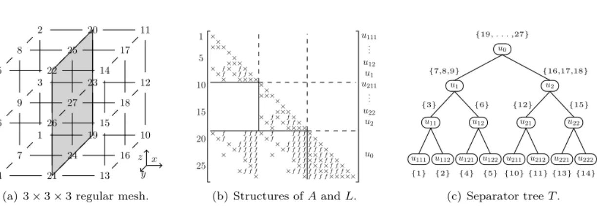
vari-ables of A according to nested dissection [9] limits the operation count and storage of sparse direct methods. We introduce a 3 × 3 × 3 domain in Figure 1(a). It is first divided by a 3 × 3 constant-x plane separator u0and each subdomain is then divided recursively. By ordering the separators after

the subdomains, large empty blocks appear in Figure 1(b). The elimination tree [12] represents the dependencies between computations. It can be compressed thanks to the use of supernodes,

x z y 1 4 2 5 10 11 13 14 3 6 12 15 7 9 8 16 18 17 19 20 21 22 23 24 25 26 27

(a) 3 × 3 × 3 regular mesh.

1 5 10 15 20 25 × × × × × × × × × × × × × × × × × × × × × × × × × × × × × × × × × × × × × × × × × × × × ×× × × × × × × × × × × × × ×× × × × ×× × × × × × ×× ×× ××× ×××× f f f f f f f f f f f f f f f f f f f fff f f f f f f f f f f f f f f f f f f f f f f f f f f f f f f f f f f f f f f f f f f f f f f f f f f f f f f f f f f fff f u0 u2 u211 u22 .. . u1 u111 .. . u12 (b) Structures of A and L. u0 u2 u22 u222 u221 u21 u212 u211 u1 u12 u122 u121 u11 u112 u111 {19, . . . ,27} {16,17,18} {15} {14} {13} {12} {11} {10} {7,8,9} {6} {5} {4} {3} {2} {1} (c) Separator tree T .

Figure 1. (a) A 3D mesh with a 7-point stencil. Mesh nodes are numbered according to a nested dissection

ordering. (b) Corresponding matrix with initial nonzeros (×) in the lower triangular part of a symmetric matrix A and fill-in (f ) in the L factor. (c) Separator tree, also showing the sets of variables to be eliminated at each node.

leading to the separator tree of Figure 1(c) when choosing supernodes identical to separators1_{. The}

order of the tree nodes (u111, u112, u11, u121, u122, u12, . . . , u0), partially represented on the right

of the matrix, is here a postordering: nodes in any subtree are processed consecutively. For u ∈ T composed of αu variables, the diagonal block associated with u in the factors matrix is formed of

two lower and upper triangular matrices L11and U11of order αu. The βunonzero off-diagonal rows

(resp. columns) below (resp. to the right of) L11 (resp. U11) can be compacted into a contiguous

matrix L21of size βu× αu(resp. U12of size αu× βu). For the example of u1 in Figure 1, αu1 = 3

(corresponding to variables 7, 8, 9), and βu1 = 9 corresponding to the off-diagonal rows 19, . . . , 27.

Starting from y ← b and from the bottom of the tree, at each node u, the active components of y can be gathered into two dense vectors y1of size αu and y2of size βu to perform the operations

(3) y1← L−111y1 and y2← y2− L21y1.

y1 and y2 can then be scattered back into y, so that y2 will be used at higher levels of T . When

the root is processed, y contains the solution of Ly = b. Denoting by δu= αu× (αu− 1 + 2βu) the

number of arithmetic operations for (3), the number of operations to solve Ly = b is

(4) ∆ =X

u∈T δu.

2. Exploitation of sparsity in right-hand sides. Consider a non-singular n × n matrix A with a nonzero diagonal, and its directed graph G(A), with an edge from vertex i to vertex j if aij 6= 0. Given a vector b, let us define struct(b) = {i, bi 6= 0} as its nonzero structure,

and closureA(b) as the smallest subset of vertices of G(A) including struct(b) without incoming

edges. Gilbert [10, Theorem 5.1] characterizes the structure of the solution of Ax = b by the relation struct(A−1b) ⊆ closureA(b), with equality in case there is no numerical cancellation. In

our context of triangular systems, ignoring such cancellation, struct(L−1b) = closureL(b) is also the

set of vertices reachable from struct(b) in G(LT), where edges have been reversed [11, Theorem 2.1]. Finding these reachable vertices can be done using the transitive reduction of G(LT), which 1_{In this example, identifying supernodes with separators leads to relaxed supernodes: the sparsity in the}

is a tree (the elimination tree) when L results from the factorization of a matrix with symmetric (or symmetrized) structure. Since we work with a tree T with possibly more than one variable to eliminate at each node, let us define Vb as the set of nodes in T including at least one element of

struct(b). The structure of L−1b is obtained by following paths from the nodes of Vbup to the root.

The tree consisting of these paths is the pruned tree of b, and we denote it by Tp(b). The number

of operations ∆ from Equation (4) now depends on b:

(5) ∆(b) = X

u∈Tp(b)

δu.

We now consider the multiple RHS case of Equation (2), where RHS columns have different structures and we denote by Bi the columns of B, for 1 ≤ i ≤ m. Rather than solving m systems

each with a different pruned tree Tp(Bi), we favor matrix-matrix computations by considering VB =S_1≤i≤mVBi, the union of all nodes in T with at least one nonzero from matrix B, and the pruned tree Tp(B) =S_1≤i≤mTp(Bi) containing all nodes in T reachable from nodes in VB. The

triangular and update operations (3) become Y1← L−111Y1 and Y2← Y2− L21Y1, leading to:

(6) ∆(B) = m × X

u∈Tp(B)

δu.

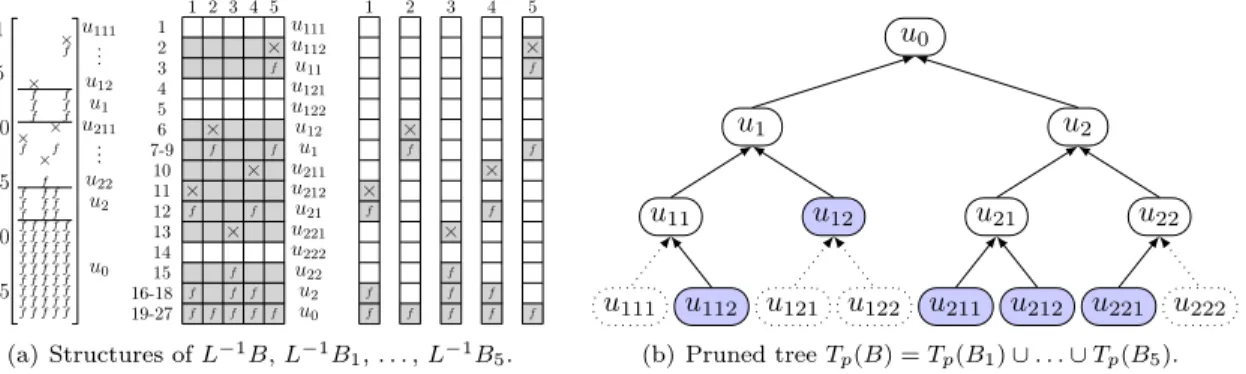
An example is given in Figure 2, where B = [{B11,1}, {B6,2}, {B13,3},{B10,4}, {B2,5}], VB =

{u212, u12, u221, u211, u112}, δ(u0) = 72, δ(u1) = δ(u2) = 60, δ(u11) = 12, δ(u112) = 6, etc.,

∆(B) = 5 × 264 = 1320, and ∆(B1) + ∆(B2) + . . . + ∆(B5) = 744. At this point, we exploit

1 5 10 15 20 25 × × × × × f f f f f f f f f f f f f f f f f f f f f f f f f f f f f f f f f f f f f f f f f f f f f f f f f f f f f f f f f f f f f f f f u0 u2 u211 u22 .. . u1 u111 u12 .. . × f f f × f f × f f f × f f f × f f f u0 u2 u22 u222 u221 u21 u212 u211 u1 u12 u122 u121 u11 u112 u111 19-27 16-18 15 14 13 12 11 10 7-9 6 5 4 3 2 1 1 2 3 4 5 1 × f f f 2 × f f 3 × f f f 4 × f f f 5 × f f f (a) Structures of L−1_{B, L}−1_B 1, . . . , L−1B5. u0 u2 u22 u222 u221 u21 u212 u211 u1 u12 u122 u121 u11 u112 u111 (b) Pruned tree Tp(B) = Tp(B1) ∪ . . . ∪ Tp(B5).

Figure 2. Illustration of multiple RHS and tree pruning. × corresponds to an initial nonzero in B and f to

“fill-in” that appears in L−1B, represented in terms of original variables and tree nodes. Gray parts of L−1B (resp. of L−1Bi) are the ones involving computations when RHS columns are processed in one shot (resp. one by one).

tree pruning, or vertical sparsity, but perform extra operations by considering globally Tp(B)

in-stead of each individual pruned tree Tp(Bi). Processing B by smaller blocks of columns would

further reduce the number of operations at the cost of more traversals of the tree and a smaller arithmetic intensity, with a minimal number of operations ∆min(B) =P_i=1,m∆(Bi) reached when B is processed column by column, as in Figure 2(a)(right). We note that performing this minimal

number of operations while traversing the tree only once (and thus accessing the L factor only once) may require performing complex and costly data manipulations at each node u with copies and indirections to work only on the nonzero entries of L−1B at u. We now present a simpler

approach which exploits the notion of intervals of columns at each node u ∈ Tp(B). This approach

to exploit what we call horizontal sparsity in B was introduced in another context [3]. Given a matrix B, we associate to a node u ∈ Tp(B) its set of active columns

(7) Zu= {j ∈ {1, . . . , m} | u ∈ Tp(Bj)} .

The interval_Jmin(Zu), max(Zu)K includes all active columns, and its length is

θ(Zu) = max(Zu) − min(Zu) + 1.

Zu is sometimes defined for an ordered or partially ordered subset R of the columns of B, in which

case we use the notation Zu|Rand θ(Zu|R). For u in Tp(B), Zu is non-empty and θ(Zu) is different

from 0. As illustrated in Figure 3, the idea is then to perform the operations (3) on the θ(Zu)

contiguous columnsJmin(Zu), max(Zu)K instead of the m columns of B , leading to

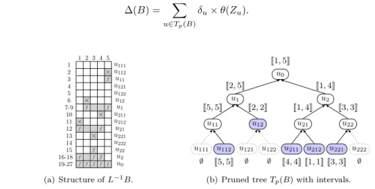
(8) ∆(B) = X u∈Tp(B) δu× θ(Zu). × f f f × f f × f f f × f f f × f f f u0 u2 u22 u222 u221 u21 u212 u211 u1 u12 u122 u121 u11 u112 u111 19-27 16-18 15 14 13 12 11 10 7-9 6 5 4 3 2 1 1 2 3 4 5 (a) Structure of L−1B. u0 u2 u22 u222 u221 u21 u212 u211 u1 u12 u122 u121 u11 u112 u111 J1, 5K J1, 4K J3, 3K ∅ J3, 3K J1, 4K J1, 1K J4, 4K J2, 5K J2, 2K ∅ ∅ J5, 5K J5, 5K ∅

(b) Pruned tree Tp(B) with intervals.

Figure 3. Column intervals for the RHS of Figure 2: in gray (a) and above/below each node (b). Taking

for instance u21, there are nonzeros in columns 1 and 4, so that Zu21 = {1, 4}. Instead of performing the solve

operations on m = 5 columns at u21, computation is limited to the θ(Zu21) = 4 columns of intervalJ1, 4K (and to a

single column at, e.g., node u221). Overall, ∆(B) is reduced from 1320 to 948 (while ∆min(B) = 744).

3. Permuting RHS columns. It is clear from Figure 3 that when exploiting horizontal

sparsity thanks to column intervals, the number of operations to solve (2) depends on the order of the columns in B. We express the corresponding minimization problem as:

(9)

Find a permutation σ of {1, . . . , m} that minimizes ∆(B, σ) =P

u∈ Tp(B)δu× θ(σ(Zu)), where σ(Zu) = {σ(i) | i ∈ Zu} , and

θ(σ(Zu)) is the length of the permuted intervalJmin(σ(Zu)), max(σ(Zu))K.

Rather than trying to solve the global problem with linear optimization techniques, we will propose a cheap heuristic based on the tree structure. We first define the notion of node optimality.

Definition 1. Given a node u in Tp(B), and a permutation σ of {1, . . . , m}, we say that we have node optimality at u, or that σ is u−optimal, if and only if θ(σ(Zu)) = #Zu, where #Zu is the cardinality of Zu. Said differently, σ(Zu) is a set of contiguous elements.

θ(σ(Zu))−#Zu, the number of columns (or padded zeros) on which extra computation is performed,

is 0 if σ is u−optimal. Using the RHS of Figure 3(a), the identity permutation is u0-optimal because

#Zu0 = #{1, 2, 3, 4, 5} = 5 = θ(Zu0), but not u1- and u2-optimal, because θ(Zu1) − #Zu1 = 2 and

θ(Zu2)−#Zu2 = 1, respectively. Our aim is thus to find a permutation σ that reduces the difference

θ(σ(Zu)) − #Zu. After describing a permutation based on a postordering of Tp(B), we present our

new heuristic, which targets node optimality in priority at the nodes near the top of the tree.

3.1. The postorder permutation. In Figure 1, the sequence [u111, u112, u11, u121, u122, u12, u1, u211, u212, u21, u221, u222, u22, u2, u0] used to order the matrix follows a postordering.

Definition 2. Consider a postordering of the tree nodes u ∈ T , and a RHS matrix B = [Bj]j=1...m where each column Bj is represented by one of its associated nodes u(Bj) ∈ VBj (see

below). B is said to be postordered if and only if: ∀j1, j2, 1 ≤ j1 < j2 ≤ m, we have either u(Bj1) = u(Bj2), or u(Bj1) appears before u(Bj2) in the postordering. In other words, the order of

the columns Bj is compatible with the order of their representative nodes u(Bj).

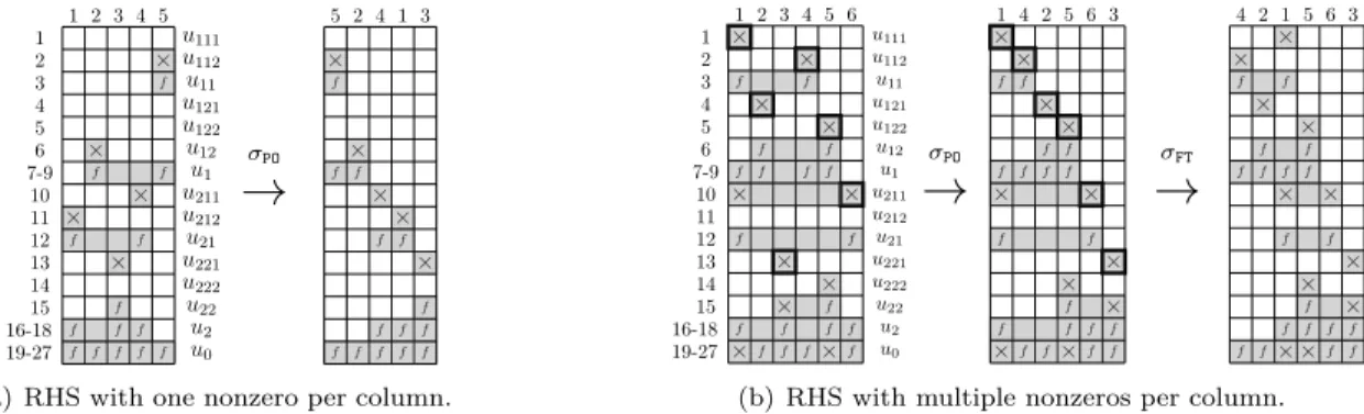
The postordering has been applied [2,15,16] to build regular chunks of RHS columns with “nearby” pruned trees, thereby limiting the accesses to the factors or the amount of computation. It was also experimented together with node intervals [3] to RHS with a single nonzero per column. In Fig-ure 3(a), B has a single nonzero per column. The initial natural order of the columns (INI) induces computation on explicit zeros represented by gray empty cells and we had ∆(B) = ∆(B, σINI) = 948

and ∆min(B) = 744 (see Figure 3). On the other hand, the postorder permutation, σPO, reorders

the columns of B so that the order of their representative nodes u112, u12, u211, u212, u221is

com-patible with the postordering. In this case, there are no gray empty cells (see Figure 4(a)) and ∆(B, σPO) = ∆min(B). More generally, it can be shown that the postordering induces no extra

computations for RHS with a single nonzero per column [3]. For applications with multiple nonze-ros per RHS, each column Bj may correspond to a set VBj with more than one node, in which case we choose the node that appears first in the sequence of postordered nodes of the tree [4]. In Figure 4(b), some columns of B have several nonzeros. For example, VB1 = {u111, u211, u0} is

× f f f × f f × f f f × f f f × f f f u0 u2 u22 u222 u221 u21 u212 u211 u1 u12 u122 u121 u11 u112 u111 19-27 16-18 15 14 13 12 11 10 7-9 6 5 4 3 2 1 1 2 3 4 5

→

(a) RHS with one nonzero per column.

× f f × f f × × f f f × × f f × f f f × f f × f f × × f f f 19-27 16-18 15 14 13 12 11 10 7-9 6 5 4 3 2 1 u0 u2 u22 u222 u221 u21 u212 u211 u1 u12 u122 u121 u11 u112 u111 1 2 3 4 5 6

→

→

(b) RHS with multiple nonzeros per column.

Figure 4. Illustration of the postordering of two RHS with one or more nonzeros per column.

represented by u111, and VB3 = {u221, u22} by u221 (cells with a bold contour). The postorder

permutation yields σPO(B) = [B1, B4, B2, B5, B6, B3], which reduces the number of gray cells and

the number of operations from ∆(B) = 1368 to ∆(B, σPO) = 1242. Computations on padded zeros

The quality of σPO depends on the tree postordering. If u111 and u112 were exchanged in the

original postordering, B1 and B4 would be swapped, further reducing ∆. One drawback of the

postorder permutation is that, since the position of a column is based a single representative node, some information is unused. In Figure 4(b), we represented another permutation σFT that yields

∆(B, σFT) = 1140. This more general and powerful heuristic is presented in the next subsection. 3.2. The flat tree permutation. With the aim of satisfying node optimality (see

Defi-nition 1), we present another algorithm to compute the permutation σ by first illustrating its geometric properties and then extending it to rely only on algebraic properties.

3.2.1. Geometrical intuition. For u ∈ T , the domain associated with u is defined by the

subtree rooted at u and is denoted by T [u]. The set of variables in T [u] corresponds to a subdomain created during the nested dissection algorithm. As an example, the initial 2D domain in Figure 5(a) (left) is T [u0] and its subdomains created by dividing it with u0are T [u1] and T [u2]. In the following, T [u] will equally refer to a subdomain or a subtree. We make the strong assumption here that the

nonzeros in an RHS column correspond to geometrically contiguous nodes in a regular domain on which a perfect nested dissection has been performed.

u0 u1 a u2 a a a b b b c c c c a b c T [u1] u1 T [u2] u2 u0 × f × × × × f

(a) Flat tree step 1.

u0 u1 u2 u12 u11 u22 u21 e d d f h g i k j l l d e f g h i j k l T [u11] T [u12] u1 T [u21] T [u22] u2 u0 × f f × × × f × f f × f × f × × × × × × × × × f × f × × f f × × × f × f f

(b) Flat tree step 2.

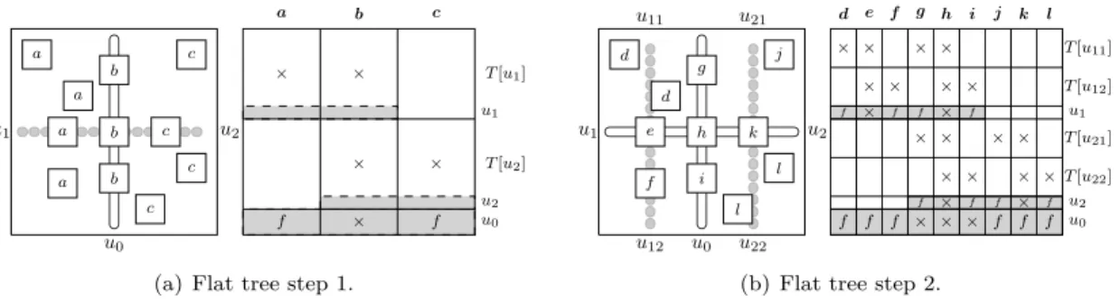
Figure 5. Flat tree geometrical illustration. In (a) and (b), the figure on the left represents different types of

RHS, and the one on the right the permuted RHS matrix. × or f in a rectangle indicate the presence of nonzeros in the corresponding submatrix, parts of the matrix filled in gray are fully dense and blank parts only contain zeros.

The flat tree algorithm relies on the evaluation of the position of each RHS column compared to separators. The name flat tree comes from the fact that, given a parent node with two child subtrees, the algorithm orders first RHS columns included in the left subtree, then RHS columns associated to the parent (because they intersect both subtrees), and finally, as in an inorder, RHS columns included in the right subtree. The RHS columns in Figure 5(a) may be identified by three different types noted a, b and c according to their positions according to the root separator u0. An

RHS column is of type a (resp. c) when its nonzero structure is included in T [u1] (resp. T [u2]),

and b when it is divided by u0. First, we group the RHS according to their type (a, b, or c) with

respect to u0 which leads to the creation of submatrices/subsets of RHS columns noted a, b and

c. Second, we make sure to place b between a and c. Since all RHS in a and b have at least one nonzero in T [u1], u1 belongs to the pruned tree of all of them, hence the dense area filled in gray

in the RHS structure. The same is true for b and c and u2. By permuting B as [a, b, c] ([c, b, a] is

also possible), a and b, and b and c, are contiguous. Thus, θ(Zu1) = #Zu1, θ(Zu2) = #Zu2 and

we have minimized (8) for u1 and u2 thanks to u1− and u2−optimality. The algorithm proceeds

l) form subsets of the RHS of a (resp. c) based on their position/type with respect to u1 (resp. u2), see Figure 5(b). Second, thanks to the perfect nested dissection assumption, u1 and u2 can

be combined to form a single separator that subdivides the RHS of b into three subsets g, h and i. During this second step, B is permuted as [d, e, f , g, h, i, j, k, l]. The algorithm stops when the tree is fully processed or the RHS sets contain a single RHS.

3.2.2. Algebraic approach. Let us consider the columns of B as an initially unordered set

of RHS columns that we denote RB = {B1, B2, . . . , Bm}. R ⊂ RB is a subset of the columns of B

and r ∈ R is a generic element of R (one of the columns Bj). A permuted submatrix of B can be

expressed as an ordered sequence of RHS columns. For two subsets of columns R and R0, [R, R0] denotes a sequence of RHS columns in which the RHS from the subset R are ordered before those from R0, without the order within R and R0 to be necessarily defined. We found this framework of RHS sets and subsets better adapted to formalize our algebraic algorithm than matrix notation with complex index permutations. We now characterize the geometrical position of a RHS using the notion of pruned layer : for a given depth d in the tree, and for a given RHS r ∈ RB, we define

the pruned layer Ld(r) as the set of nodes at depth d in the pruned tree Tp(r). In the example of

Figure 5(a), L1(r) = {u1} for all r ∈ a, L1(r) = {u2} for all r ∈ c, and L1(r) = {u1, u2} for all r ∈ b. The notion of pruned layer formally identifies sets of RHS with common characteristics in

the tree, without geometric information. This is formalized and generalized by Definition 3. Definition 3. Let R ⊂ RB be a set of RHS, and let U be a set of nodes at depth d of the tree T . We define R[U ] = {r ∈ R | Ld(r) = U } as the subset of RHS with pruned layer U .

We have for example, see Figure 5: R[{u1}] = a, R[{u2}] = c and R[{u1, u2}] = b at depth d = 1.

The algebraic recursive algorithm is depicted in Algorithm 1. Its arguments are R, a set of RHS and d, the current depth. Initially, d = 0 and R = RB = R[u0]. At each recursion step, the

algorithm builds the distinct pruned layers Ui = Ld+1(r) for the RHS r in R. Then, instead of

looking for a permutation σ to minimizeP

u∈Tp(RB)δu×θ(σ(Zu)), it orders the R[Ui] by considering the restriction of (9) to R and to nodes at depth d + 1 of Tp(R). Furthermore, with the assumption

that T is balanced, all nodes at a given level of Tp(R) are of comparable size. δu may thus be

assumed constant per level and needs not be taken into account. The algorithm is a greedy top-down algorithm, where at each step a local optimization problem is solved. This way, priority is given to the top of the tree, which is in general more critical because factor matrices are larger.

Algorithm 1 Flat Tree procedure Flattree(R, d)

1) Build the set of children C(R)

1.1) Identify the distinct pruned layers (pruned layer = set of nodes) U ← ∅

for all r ∈ R do

U ← U ∪ {Ld+1(r)} end for

1.2) C(R) = {R[U ] | U ∈ U }

2) Order children C(R) as [R[U1], . . . , R[U#C(R)]]:

return [Flattree(R[U1], d + 1),. . .,Flattree(R[U#C(R)], d + 1)] end procedure

follows: each node R of Trec represents a set of RHS, C(R) denotes the set of children of R and

the root is RB. By construction of Algorithm 1, C(R) is a partition of R, i.e., R = ˙S_R0_∈C(R)R0

(disjoint union). Note that all r ∈ R such that Ld+1(r) = ∅ belong to R[∅], which is also included

in C(R). In this special case, R[∅] can be added at either extremity of the current sequence without introducing extra computation and the recursion stops for those RHS, as will be illustrated in Figures 6 and 7(a). With this construction, each leaf of Trec contains RHS with indistinguishable

nonzero structures, and keeping them contiguous in the final permutation avoids introducing extra computations. Assuming that for each R ∈ Trec the children C(R) are ordered, this induces an

ordering of all the leaves of the tree, which defines the final RHS sequence. We now explain how the set of children C(R) is built and ordered at each step:

1) Building the set of children. The set of children of R ∈ Trec is built by first identifying

the pruned layers U of all RHS r ∈ R. The different pruned layers are stored in U and we have for example (Figure 5, first step of the algorithm), U = {{u1}, {u2}, {u1, u2}}. We define C(R) = {R[U ] | U ∈ U } (Definition 3), which forms a partition of R. One important property is

that all r ∈ R[U ] have the same nonzero structure at the corresponding layer so that numbering them contiguously prevents the introduction of extra computation.

2) Ordering the children. The children sequence [R[U1], . . . , R[U#C(R)]] at depth d + 1 should

minimize the size of the intervals for nodes u at depth d + 1 of Tp(R). The order inside each R[Ui] does not impact the size of these intervals (it will only impact lower levels). For any node u at depth d + 1 in Tp(R), we have θ(Zu|R) = max(Zu|R) − min(Zu|R) + 1 = P

imax(u)

i=imin(u)#R[Ui],

where Zu|R is the set of permuted indices representing the active columns restricted to R, and imin(u) = min{i ∈ {1, . . . , #C(R)} | u ∈ Ui} (resp. imax(u) = max{i ∈ {1, . . . , #C(R)} | u ∈ Ui})

is the first (resp. last) index i such that u ∈ Ui. Finally, we minimize the local cost function (sum

of the interval sizes for each node at depth d + 1):

(10) cost([R[U1], . . . , R[U#C(R)]]) = X u∈Tp(R) depth(u)=d+1 imax(u) X

i=imin(u) #R[Ui]

To build the ordered sequence [R[U1], . . . , R[U#C(R)]], we use a greedy algorithm that starts with

an empty sequence, and at each step k ∈ {1, . . . , #C(R)} inserts a RHS set R[U ] picked randomly in C(R) at the position that minimizes (10) on the current sequence. To do so, we simply start from one extremity of the sequence of size k − 1 and compute (10) for the new sequence of size k for each possible position 0 . . . k; if several positions lead to the same minimal cost, the first one encountered is chosen. In case u−optimality is obtained for each node u considered, then the permutation is said to be perfect and the cost function is minimal, locally inducing no extra operations on those nodes. Figure 6 shows the recursive structure of the RHS sequence after applying the algorithm on a binary tree. We refer to this representation as the layered sequence. For simplicity, the notation for pruned layers has been reduced from, e.g., {u1} to u1, and from {u1, u2} to u1u2. From the recursion tree

point of view, R[u1], R[u1u2], R[u2] are the children of R[u0] in Trec, R[u11], R[u11u12], R[u12] the

ones of R[u1], etc.

Although we still use a binary tree, we make no assumption on the RHS structure, the domain, or the ordering in the example of Figure 7. The set of pruned layers corresponding to R[u0] is

U = {u1u2, u1, ∅, u2}, so that C(R[u0]) = {R[u1u2], R[u1], R[∅], R[u1u2]}. As can be seen in the

non-permuted RHS structure, R[∅] = B4at depth 1 induces extra operations at nodes descendants

R[u0]

d = 0

R[u1] R[u1u2] R[u2]

d = 1

R[u11] R[u11u12] R[u12] ∗ R[u21] R[u21u22] R[u22]

d = 2

Figure 6. A layered sequence built by the flat tree algorithm on a binary tree. Sets R[∅] (not represented) could

be added at either extremity of the concerned sequence (e.g., right after R[u2] for a RHS included in u0). With the

strong assumptions of Figure 5, * = R[u11u21], R[u11u12u21u22], R[u12u22]. Otherwise, * is more complex.

× × × f f f f × × × × × × × f f × f × f f × f × f f u0 u2 u22 u21 u1 u12 u11 1 2 3 4 5 6 7 σFT f f × × × × × × f × f f × × × f f × f × f f × f f × 2 3 6 1 7 5 4 (a) RHS structure. u0 u2 u22 u21 u1 u12 u11 (b) Separator tree T . R[u0] B1, . . . , B7 R[u1u2] B1B3B6B7 R[u11u22] B7 R[u21u22] B1 R[u12u21] B6 R[u12] B3 R[u1] B2 R[u2] B5 R[∅] B4

(c) Recursion tree Trec.

Figure 7. Illustration of the algebraic flat tree algorithm on a set of 7 RHS.

last and obtain the sequence [R[u1], R[u1u2], R[u2], R[∅]]. A recursive call is done on the identified

sets, as illustrated in Figure 7(c). Since R[u1], R[u2] and R[∅] contain a single RHS, we focus

on R = R[u1u2], whose set of pruned layers is U = {u21u22, u12, u12u21, u11u22}. The sequence

[R[U1], R[U2], R[U3], R[U4]], where U1 = u12, U2 = u12u21, U3 = u21u22, and U4 = u11u22 is

a perfect sequence which gives local optimality. However, taking the problem globally, we see that θ(Zu11) 6= #Zu11 in the final sequence [B2, B3, B6, B1, B7, B5, B4]. Although not relying on

geometric assumptions, particular RHS structures or binary trees, computations on explicit zeros (for example zero rows in column f and subdomain T [u11] in Figure 5(b)), may still occur with the

flat tree algorithm. This will also be illustrated in Section 5, where ∆(B, σFT) is 39% larger than

∆min(B), in the worst case. A blocking algorithm is now introduced to further reduce ∆(B, σFT). 4. Toward a minimal number of operations using blocks.

4.1. Geometrical intuition. In terms of operation count, optimality (∆min(B)) is obtained when processing the columns of B one by one, using m blocks. However, this requires processing the tree m times and will typically lead to a poor arithmetic intensity (and likely a poor performance). On the other hand, the algorithms of Section 3 only use one block, which provides a higher arithmetic intensity but requires extra operations. In this section, our objective is to create a minimal number of (possibly large) blocks while reducing the number of extra operations by a given amount.

On the one hand, two RHS or sets of RHS included in two different domains exhibit interesting properties, as can be observed for sets a ∈ T [u1] and c ∈ T [u2] from Figure 5(a). No extra

operations are introduced between them: ∆([a, c]) = ∆(a) + ∆(c). We say that a and c are

independent sets and they can be associated together. On the other hand, a set of RHS intersecting

(a and c) which will likely introduce extra computation. In Figure 5(b), we have for example ∆([a, b]) = ∆([d, e, f , g, h, i]) > ∆([d, e, f ]) + ∆([g, h, i]) = ∆(a) + ∆(b) and ∆([a, b, c]) > ∆(a) + ∆(b) + ∆(c). We say that b is a set of problematic RHS. Figure 4 (right) gives another example where extracting the problematic RHS B1and B5from [B4, B2, B1, B5, B6, B3] suppresses

all extra operations: ∆([B4, B2, B6, B3]) + ∆([B1, B5]) = ∆min = 1056. Situations where no

assumption on the RHS structure is made are more complicated and require a general approach. For this, we formalize the notion of independence, which will be the basis for our blocking algorithm.

4.2. Algebraic formalization. In this section, we assume the matrix B to be flat tree ordered

and the recursion tree Trec to be built and ordered. Using the notations of Definition 3, we give an

algebraic definition of the independence property:

Definition 4. Let U1, U2be two sets of nodes at a given depth of a tree T , and let R[U1], R[U2] be the corresponding sets of RHS. R[U1], R[U2] are said to be independent if and only if U1∩U2= ∅.

With Definition 4, we are able to formally identify independent sets that can be associated together. Take for example a = R[u1] and c = R[u2] (Figure 5(a)), R[u1] and R[u2] are independent and

∆([R[u1], R[u2]]) = ∆(R[u1]) + ∆(R[u2]). On the contrary, when R[U1], . . . , R[Un] are not pairwise

independent, we group together independent sets of RHS, while forming as few groups as possible. This problem is equivalent to a graph coloring problem, where R[U1], . . . , R[Un] are the vertices

and an edge exists between R[Ui] and R[Uj] if and only if Ui∩ Uj 6= ∅. Several heuristics exist

for this problem, and each color will correspond to one group. The blocking algorithm as depicted

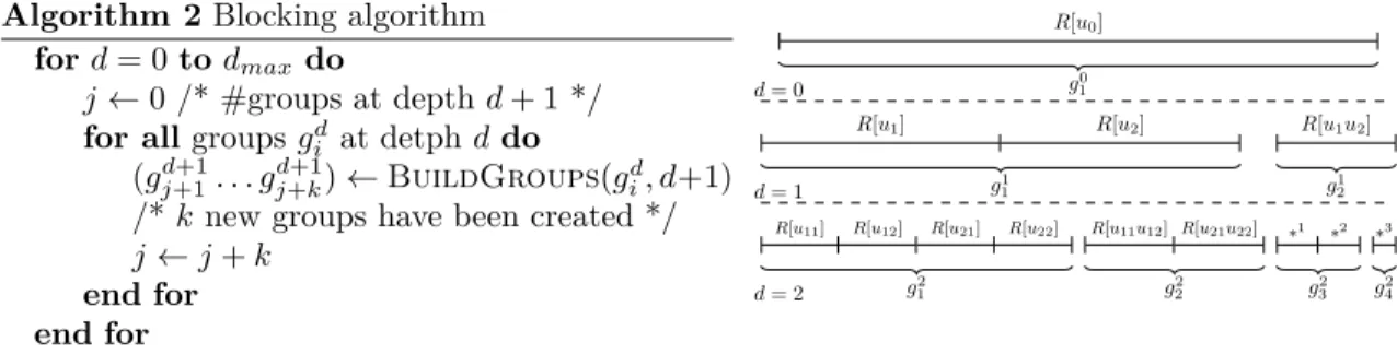
Algorithm 2 Blocking algorithm for d = 0 to dmax do

j ← 0 /* #groups at depth d + 1 */ for all groups gd

i at detph d do

(gd+1_j+1. . . g_j+kd+1_{) ← BuildGroups(g}d i, d+1)

/* k new groups have been created */

j ← j + k end for end for R[u0] g0 1 d = 0

R[u1] R[u2] R[u1u2]

g1

1 g12

d = 1

R[u11] R[u12] R[u21] R[u22]

g2 1 R[u11u12] R[u21u22] g2 2 ∗1 _∗2 g2 3 ∗3 g2 4 d = 2

Figure 8. A first version of the blocking algorithm (left). It is illustrated (right) on the layered sequence of

Figure 6. With the geometric assumptions of Figure 5, ∗1_{= R[u}

11u21], ∗2= R[u12u22], and ∗3= R[u11u12u21u22].

in Figure 8 traverses Trec from top to bottom. At each depth d, each intermediate group gid

verifies the following properties: (i) gd

i can be represented by a sequence [R[U1], . . . , R[Un]], and

(ii) the sequence respects the flat tree order of Trec. Then, BuildGroups(gdi, d + 1) first builds

the sets of RHS at depth d + 1, which are exactly the children of the R[Uj] ∈ gid in Trec. Second,

BuildGroups(gdi, d + 1) solves the aforementioned coloring problem on these RHS sets and builds

the k groups (g_j+1d+1, . . . , g_j+kd+1).

In Figure 8(right), there is initially a single group g0

1 = [R[u0]] with one set of RHS, which may

be expressed as the ordered sequence [R[u1]R[u1u2]R[u2]]. g10 does not satisfy the independence

property at depth 1 because u1∩ u1u2 6= ∅ or u2∩ u1u2 6= ∅. BuildGroups(g10, 1) yields g11 =

[R[u1], R[u2]] and g12= [R[u1u2]]. The algorithm proceeds until a maximal depth dmax: (g21, g22) =

(ii), let us take sets d = R[u11], f = R[u12], j = R[u21] and l = R[u22] from Figure 5(b). One

can see that ∆([d, f , j, l]) = ∆(d) + ∆(f ) + ∆(j) + ∆(l) < ∆([d, j, f , l]). Compared to [d, f , j, l] which respects the global flat tree ordering and ensures u1- and u2-optimality, [d, j, f , l] does not

and would thus increase θ(Zu1) and θ(Zu2). Furthermore, Algorithm 2 ensures the property (whose

proof can be found in [4]), that the independent sets of RHS grouped together do not introduce extra operations:

Property 5. For any group gd = [R[U1], . . . , R[Un]] created through Algorithm 2 at depth d, we have ∆([R[U1], . . . , R[Un]]) =P

n

i=1∆(R[Ui]).

Interestingly, Property 5 can be used to prove, in the case of a single nonzero per RHS, the optimality of the flat tree permutation.

Corollary 6. Let RB be a set of RHS such that ∀r ∈ RB, #Vr = 1. Then the flat tree permutation is optimal: ∆(RB) = ∆min(RB).

Proof. Since ∀r ∈ RB, #Vr = 1, Tp(r) is a branch of T . As a consequence, any set of RHS R[U ] built through the flat tree algorithm is represented by a pruned layer U containing a single

node u. At each step of the flat tree algorithm (Algorithm 1), the RHS sets identified are thus all independent from each other. When applying Algorithm 2, a unique group RB is then kept until

the bottom of the tree. Blocking is thus not needed and Property 5 applies at each level of the recursion. ∆(RB) is thus equal to the sum of the ∆(R[U ]) for all leaves R[U ] of the recursion tree Trec. Since ∆(R[U ]) = ∆min(R[U ]) on those leaves (all RHS in R[U ] involve the exact same nodes

and operations), we conclude that ∆(RB) = ∆min(RB).

This proof is independent of the ordering of the children at step 2 of Algorithm 1. Corollary 6 is thus more general: any top-down recursive ordering keeping together RHS with identical pruned layer at each step is optimal, as long as the pruned layers identified at each step are independent.

R[u1] R[u2]

g1 1

d = 1

R[u11] R[u12] R[u21] R[u22]

g2 1 R[u11u12] R[u21u22] g2 2 d = 2 R[u1] R[u2] g1 1 d = 1

R[u11] R[u12] R[u21u22]

g2 1

R[u21] R[u22] R[u11u12]

g2 2

d = 2

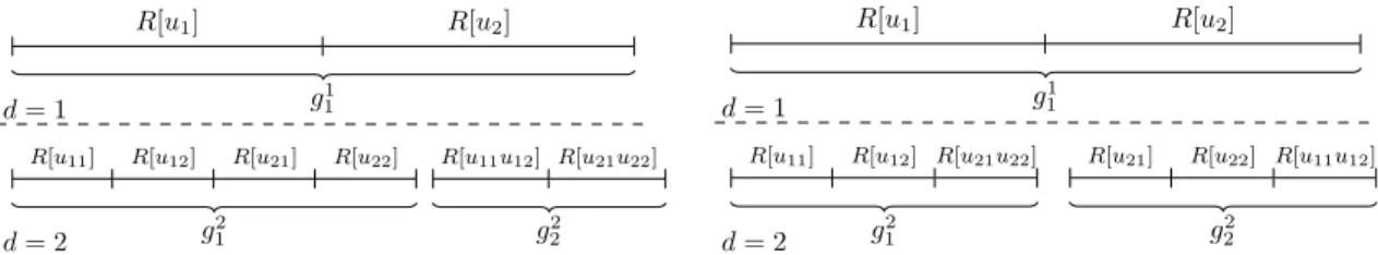
Figure 9. Two strategies to build groups: CritPathBuildGroups (left) and RegBuildGroups (right).

Back to the BuildGroups function, the solution of the coloring problem may not be unique. Even on the simple example of Figure 8, there are several ways to define groups, as shown in Figure 9 for g1

1: both strategies satisfy the independence property and minimize the number of

groups. The CritPathBuildGroups strategy tends to create a large group g2

1 and a smaller one, g2

2. In each group the computations on the tree nodes are expected to be well balanced because

all branches of the tree rooted at u0 might be covered by the RHS (assuming thus a reasonably

balanced RHS distribution over the tree). The choice of CritPathBuildGroups can be driven by tree parallelism considerations, namely, the limitation of the sum of the operation counts on the critical paths of all groups. The RegBuildGroups strategy tends to balance the sizes of the groups but may create more unbalance regarding the distribution of work over the tree.

necessary, and that for a given group, enforcing the independence property may create more than two groups. In the next section we minimize the number of groups created using greedy heuristics.

4.3. A greedy approach to minimize the number of groups. Compared to Algorithm 2,

Algorithm 3 adds the group selection, limits the number of groups created from a given group to two, and stops depending on a given tolerance on the amount of operations.

First, instead of stepping into each group as in Algorithm 2, we select among the current groups the one responsible for most extra computation, that is, the one maximizing ∆(g) − ∆min(g). This

implies that groups that are candidate for splitting might have been created at different depths and we use a superscript to indicate the depth d at which a group was split, as in the notation g₀d.

Second, instead of a coloring problem which creates as many groups as colors obtained, we look (procedure BuildMaxIndepSet) inside the RHS sets of gd0 for a maximal group of independent

sets at depth d + 1, denoted gd+1_imax. The other sets are left in another group gdc, whose depth remains

equal to d. gcdmay thus consist of dependent sets that may be subdivided later if needed2. Rather

than an exact algorithm to determine gd+1_imax, we use a greedy heuristic.

Finally, we define µ0 as the tolerance of extra operations authorized. With a typical value µ0 = 1.01, the algorithm stops when the number of extra operations is within 1% of the minimal

number of operations ∆min, returning G as the final set of groups. Algorithm 3 Blocking algorithm

G ← {RB}, ∆min← ∆min(RB), ∆ ← ∆(RB) while ∆/∆min> µ0do

Select gd

0 such that ∆(gd0) − ∆min(gd0) = maxg∈G(∆(g) − ∆min(g)) . Group selection

(g_imaxd+1 , gd c) ← BuildMaxIndepSet(g0d, d+1) G ← G ∪ {g_imaxd+1 , g_cd} \ {gd 0} ∆ ← ∆ − ∆(g₀d) + ∆(g_imaxd+1 ) + ∆(gd_c) end while

5. Experimental results. In this section, we report on the impact of the proposed

permuta-tion and blocking algorithms on the forward substitupermuta-tion (Equapermuta-tion (2)), using a set of 3D regular finite difference problems coming from seismic and electromagnetism modeling [1,14], for which the solve phase is costly. The characteristics of the corresponding matrices and RHS are presented in Table 1. In both applications, the nonzeros of each RHS correspond to a small set of close points, near the top of the 3D grid corresponding to the physical domain, with some overlap between RHS. Except in Section 5.3, a geometric nested dissection (ND) algorithm is used to reorder the matrix.

5.1. Impact of the flat tree algorithm. We first introduce the terminology used to denote

the different strategies developed in this study and that impact the number of operations ∆. DEN represents the dense case, where no optimization is used to reduce ∆, and TP means tree pruning. When column intervals are exploited at each tree node, we denote by RAN, INI, PO and FT the random, initial (σ = id), postorder (σPO) and flat tree (σFT) permutations, respectively.

The improvements brought by the different strategies are presented in Table 2. Compared to the dense case, TP divides ∆ by at least a factor 2. When column intervals are exploited at each node, the large gap between RAN and INI shows that the original column order holds geometrical properties. FT behaves better than INI and PO and gets reasonably close to ∆min. Overall, FT

2_{In case g}d

Table 1

Characteristics of the n × n matrix A and n × m matrix B for different test cases. D(A) = nnz(A)/n and D(B) = nnz(B)/m represent the average column densities for A and B, respectively.

application matrix n(×106_{) D(A) sym m D(B)}

seismic modeling 5Hz 2.9 24 no 2302 567 7Hz 7.2 25 no 2302 486 10Hz 17.2 26 no 2302 486 electro-magnetism modeling H0 .3 13 yes 8000 9.8 H3 2.9 13 yes 8000 7.5 H17 17.4 13 yes 8000 6 H116 116.2 13 yes 8000 6 S3 3.3 13 yes 12340 19.7 S21 20.6 13 yes 12340 9.5 S84 84.1 13 yes 12340 8.6 D30 29.7 23 yes 3914 7.6 Table 2

Number of operations (×1013_{) during the}

forward substitution (LY = B) according to

the strategy used (ND ordering).

∆ DEN TP RAN INI PO FT ∆min

5Hz 1.73 .74 .74 .44 .36 .28 .22 7Hz 5.94 2.54 2.52 1.46 1.21 .92 .69 10Hz 20.62 9.01 8.92 4.78 3.85 2.87 2.26 H0 .39 .11 .11 .086 .070 .057 .050 H3 7.19 3.33 3.31 2.48 1.47 1.26 .95 H17 81.34 37.15 36.97 27.52 10.41 10.21 10.12 H116 990.02 448.31 445.91 327.89 123.79 121.76 120.68 S3 13.36 4.98 4.91 3.73 2.65 2.17 1.71 S21 156.20 49.04 48.07 35.42 25.73 22.53 19.43 S84 983.48 286.57 282.70 222.59 161.87 138.56 118.51 D30 71.60 39.78 39.38 19.49 10.93 10.21 7.31 Table 3

Theoretical tree parallelism according to the strategy used (ND ordering).

S DEN TP RAN INI PO FT

5Hz 8.60 3.91 3.88 3.11 2.39 2.54 7Hz 8.92 3.97 3.94 3.02 2.25 2.48 10Hz 9.10 4.04 4.02 2.96 2.30 2.30 H0 5.88 2.11 2.11 1.75 1.51 1.45 H3 5.99 3.22 3.21 2.47 2.02 2.11 H17 6.32 3.34 3.32 2.54 2.00 1.97 H116 7.92 3.63 3.61 2.75 2.05 2.02 S3 6.12 2.84 2.83 2.18 1.73 1.61 S21 6.30 2.56 2.46 1.85 1.49 1.47 S84 8.01 2.41 2.38 1.90 1.53 1.52 D30 8.50 4.73 4.70 2.86 2.05 2.56 Table 4

Impact of the number of groups NG on the nor-malized operation count, until ∆N G/∆min becomes

smaller than the tolerance µ0= 1.01 (ND ordering).

∆N G/∆min FT NG= 2 NG= 3 NG= 4 NG= 5 5Hz 1.283 1.111 1.001 x x 7Hz 1.321 1.116 1.002 x x 10Hz 1.269 1.029 1.002 x x H0 1.148 1.029 1.010 1.002 x H3 1.329 1.068 1.027 1.005 x H17 1.009 x x x x H116 1.009 x x x x S3 1.275 1.120 1.045 1.012 1.003 S21 1.160 1.037 1.015 1.003 x S84 1.169 1.041 1.015 1.002 x D30 1.397 1.082 1.058 1.024 1.004

provides a 13% gain on average over PO. However, the gain on ∆ decreases from 25% on the 10Hz problem to 1% on the H116 problem. This can be explained by the fact that B is denser for the seismic applications than for the electromagnetism applications (see Table 1). Indeed, the sparser

B, the closer we are to a single nonzero per RHS in which case both FT and PO are optimal.

Second, we evaluate the impact of exploiting RHS sparsity on tree parallelism. Table 3 gives the maximal theoretical speed-up S that can be reached using tree parallelism only (node parallelism is also needed, for example on the root). It is defined as S = ∆/∆cp where ∆cp is the number

of operations on the critical path of the tree. We observe that, when sparsity is exploited, tree parallelism is significantly smaller than in the dense case. This is because the depth of the pruned tree Tp(B) is similar to that of the original tree (some nonzeros of B generally appear in the leaves),

while the tree effectively processed is pruned and thus the overall amount of operations is reduced. For the same reason, S is smaller for test cases where D(B) is small. For the 5Hz, 7Hz, and 10Hz problems which have more nonzeros per column of B, besides decreasing the operation count more than the other strategies, FT exhibits equivalent or even better tree parallelism than PO. For such matrices, where D(B) is large, FT balances the work on the tree better than PO and reduces the work on the critical path more than the total work. Overall, FT reduces the operation count better

than any other strategy and has good parallel properties.

5.2. Impact of the blocking algorithm. First, we show that the blocking algorithm

de-creases the operation count ∆ while creating a small number of groups. Second, we discuss parallel properties of the clustering strategies illustrated in Figure 9. In Table 4, we report the value of ∆N G/∆min as a function of the number of groups created. x means that the blocking algorithm

stopped because the condition ∆N G/∆min ≤ µ0was reached, with µ0 for Algorithm 3 set to 1.01.

Computing from Table 4 the ratio of extra operations reduction 1 − ∆N G−∆min

∆1−∆min for N G groups created, we observe an average reduction of 74% of the extra operations when N G = 2, i.e., when only two groups are created. Table 4 also shows that ∆N G reaches a value close to ∆min very

quickly.

Table 5

Sum of critical paths’ operations (×1013_{) for two grouping strategies when three groups are created.}

P

g∆cp(g) 5Hz 7Hz 10Hz H0 H3

CritPathBuildGroup .092 .30 1.00 .037 .50 RegBuildGroup .12 .43 1.58 .044 .72

In Table 5, we report the sum of operation counts on the critical paths ∆cpover all groups

cre-ated using CritPathBuildGroup and RegBuildGroup strategies, when the number of groups created is three, leading to a value ∆ close to ∆min, see column “NG=3” of Table 4. In this case, the

total number of operations ∆ during the forward solution phase on all groups is equal whether we use CritPathBuildGroup or RegBuildGroup. Tree parallelism is thus a crucial discriminant between both strategies, and we indeed observe in Table 5 that CritPathBuildGroup effectively limits the length of critical paths over the three groups created, justifying its use.

5.3. Experiments with other orderings. As mentioned earlier, several orderings may be

used to order the unknowns of the original matrix, thanks to the algebraic nature of our flat tree and blocking algorithms. Although local ordering methods (AMD, AMF as provided by the MUMPS package3) are known not to be competitive with respect to algebraic nested dissection-based approaches such as SCOTCH4or METIS5on large 3D problems, we include them in Table 6 in order to study how the flat tree and blocking algorithms behave in general situations.

First, an important aspect of using other orderings is that they often produce much more irregular trees, leading to a large number of pruned layers to sequence. The FT permutation reduces the operation count significantly with SCOTCH and METIS, for which we observe an average 31% and 26% reduction compared to the PO permutation. Gains are also obtained with AMD for most test cases. However, FT does not perform well with AMF. This can be explained by the fact that AMF produces too irregular trees which do not fit well with our design of the FT strategy.

Second, we evaluate the blocking algorithm (BLK) and compare it with a regular blocking algorithm (REG) based on the PO permutation, that divides the initial set of columns into regular chunks of columns. Table 6 shows that the number of groups required to reach ∆/∆min ≤ 1.01 is

much smaller for BLK than for REG in all cases. Our blocking algorithm is very efficient with most orderings except AMF, where the number of groups created is high (but still lower than REG).

3_{http://mumps.enseeiht.fr/}

4_{http://www.labri.fr/perso/pelegrin/scotch/}

Table 6

Operation count ∆(×1013_{) for permutation strategies PO and FT, and number of groups NG required to reach} ∆N G

∆min ≤ 1.01 for blocking strategies REG and BLK. Different orderings (AMD, AMF, SCOTCH, METIS) are used.

AMD AMF SCOTCH METIS

σ PO REG FT BLK ∆min PO REG FT BLK ∆min PO REG FT BLK ∆min PO REG FT BLK ∆min

∆ NG ∆ NG ∆ NG ∆ NG ∆ NG ∆ NG ∆ NG ∆ NG 5Hz 1.44 53 1.36 4 1.25 .75 51 .87 7 .68 .47 328 .32 3 .25 .43 230 .30 3 .24 7Hz 5.03 38 4.44 4 4.35 15.3 18 17.8 12 14.9 1.60 287 1.14 3 .86 1.42 230 1.08 3 .82 10Hz 19.3 154 19.8 3 15.3 96.9 253 99.1 11 82.1 5.86 288 4.21 3 3.05 4.67 281 3.44 3 2.53 H0 .54 533 .53 4 .47 .12 333 .12 5 .091 .073 499 .063 3 .055 .077 615 .067 3 .057 H3 135 380 106 5 9.07 101 63 134 17 9.26 2.19 615 1.76 5 1.18 1.95 533 1.53 5 1.12 H17 183 266 226 7 136 467 173 558 50 396 22.8 380 19.0 5 12.6 21.49 242 16.8 4 12.3 H116 2244 1 2244 1 2244 39383 1 39384 1 39383 291 109 224 4 153 264 78 215 4 157 S3 20.9 725 17.9 6 15.1 20.7 184 24.8 10 17.8 4.5 771 3.41 5 2.72 3.24 771 2.64 5 2.09 S21 393 685 349 5 311 1141 493 1352 77 831 50.9 492 39.6 4 31.7 34.3 223 28.5 5 24.9 S84 3025 352 2848 5 2501 38664 725 45346 213 30977 289 286 228 4 193 207 171 174 4 151 D30 115 111 121 8 94.5 1015 139 1280 75 825 16.7 156 12.8 5 8.77 15.5 144 13.0 5 8.61

5.4. Performance. We analyse in this section the time for the forward substitution and for

the flat tree and blocking algorithms on a single Intel Xeon core @2.2GHz. A performance analysis in multithreaded or distributed environment for the largest problems is out of the scope of this study. In Table 7, we report the time of the forward substitution of the MUMPS solver6_{and the percentage}

of time spent in BLAS operations, excluding the time for data manipulation and copies. Timings with the regular blocking REG to reach our target number of operations (∆N G/∆min ≤ 1.01), at

the cost of a larger number of groups, N G  1, are also indicated.

Table 7

Time (seconds) of the forward substitution according to the strategy used and number of groups NG created with BLK and REG (ND ordering). The percentage of actual computation time (BLAS) is indicated in parentheses.

DEN TP INI PO REG FT BLK NGBLK NGREG

5Hz 3132 (34) 561 (80) 305 (88) 246 (89) 429 (95) 190 (89) 148 (91) 3 328 7Hz 9101 (40) 1727 (89) 951 (93) 784 (94) 1137 (97) 594 (94) 460 (95) 3 255 H0 862 (58) 161 (82) 125 (85) 97 (89) 88 (96) 79 (89) 67 (92) 4 328 H3 12419 (72) 4478 (92) 3274 (94) 1901 (96) 1709 (98) 1624 (96) 1234 (97) 4 306 S3 26328 (64) 6839 (89) 5005 (92) 3429 (95) 3450 (99) 2804 (96) 2195 (97) 5 536

Table 7 shows that the time reduction is in agreement with the operations reduction reported in Table 2. One can also notice that when exploiting sparsity, the proportion of time spent in BLAS operations increases. This is due to the fact that the relative weight of the top of the tree (with larger fronts for which time is dominated by BLAS operations) is larger when sparsity is exploited. When targeting a reduction of the number of operations with a regular blocking (REG), the large number of blocks (last column of Table 7) makes the granularity of the BLAS operations too small to reach the performance of the BLK strategy. On the other hand, Table 8 shows that larger regular blocks improve the Gflop rate but are not competitive with respect to BLK because of the increase in the number of operations. We also observe that the best block size for REG is problem-dependent. Table 9 relates the execution time of the flat tree and blocking algorithms. The execution times are reasonable compared to the corresponding execution time of the forward substitution. Moreover,

Table 8

Operation count (×1013_{) and time (seconds) of REG}

for different block sizes.

REG 64 128 256 512 1024 ∆ Ts ∆ Ts ∆ Ts ∆ Ts ∆ Ts 5Hz .24 188 .25 179 .27 188 .27 188 .31 209 7Hz .74 558 .78 538 .86 575 .93 611 .98 643 H0 .051 77 .051 74 .052 72 .054 74 .058 79 H3 .98 1447 1.02 1405 1.04 1369 1.09 1407 1.16 1499 S3 1.75 2533 1.78 2448 1.80 2358 1.86 2379 1.91 2424 Table 9

Time (seconds) of the flat tree and blocking algo-rithms for different orderings.

ND AMD AMF SCOTCH METIS

FT BLK FT BLK FT BLK FT BLK FT BLK 5Hz .77 .11 .64 .19 1.35 .34 .79 .20 1.02 .13 7Hz 1.30 .30 1.56 .62 5.68 3.9 1.85 .56 2.48 .34 H0 .09 .04 1.72 .04 .13 .04 .09 .02 .12 .04 H3 .52 .26 1.56 .29 1.15 3.0 .55 .24 1.15 .54 S3 .88 .33 2.20 .41 2.51 1.3 .84 .36 1.75 .49

we observe that the time of the flat tree algorithm only slowly increases with the problem size. The time of the blocking algorithm, due to its limited number of iterations, is not critical.

6. Guided Nested Dissection. Given an ordering and a tree, one may think of moving the

unknowns corresponding to RHS nonzeros to supernodes higher in the tree with on the one hand, a smaller pruned tree, but on the other hand, an increase in the factor size due to larger supernodes. Better, one may guide the ordering to include as many nonzeros of B as possible within separators during the top-down nested dissection and prune larger subtrees. This will however involve a significant extra cost for applications where each RHS contains several contiguous nodes in the grid, e.g., form a small parallelepiped. For such applications, the geometry of the RHS nonzeros could however be exploited. A first idea avoids problematic RHS by choosing separators that do not intersect RHS nonzeros. Although this idea could be tested by adding edges between RHS nonzeros before applying SCOTCH or METIS, this does not appear to be so useful in our applications, where we observed significant overlap between successive RHS. Another idea, when all RHS are localized in a specific area of the domain, is to shift the separators from the nested dissection to insulate the RHS in a small part of the domain. Such a modification of the ordering yields an unbalanced tree in which the RHS nonzeros appear at the smaller side of the tree, improving the efficiency of tree pruning and resulting in a reduction of ∆min, and thus ∆. This so called guided nested dissection

was implemented and tested on the set of test cases shown in Table 10, where we observe that the number of operations ∆min is decreased, as expected. Since the factor size has also increased

significantly, a trade-off may be needed to avoid increasing too much the cost of the factorization.

Table 10

Number of operations ∆minand factor size for original (ND) and guided (GND) nested dissection orderings.

Matrices 5Hz 7Hz 10Hz H0 H3

Strategy ND GND ND GND ND GND ND GND ND GND ∆min(×1013) .22 .19 .69 .62 2.26 1.99 .050 .025 .95 .81

factor size (×109_{) 3.72 5.18 12.8 19.7 44.8 73.4 .24 .37 4.50 5.57}

7. Applications and related problems. We describe applications where our contributions

can be applied. When only part of the solution is needed, one can show that the approaches described in Section 2 can be applied to the backward substitution (U X = Y ), which involves similar mechanisms as the forward substitution [15, 17]. The backward substitution traverses the tree nodes from top to bottom so that the interval mechanism is reversed, i.e., the interval from a parent includes the intervals from its children and the properties of local optimality are preserved. If the structure of the partial solution requested differs from the RHS structure, another call to