A Comparative Study of Mel Cepstra and EIH for Phone
Classification under Adverse Conditions
by
Sumeet Sandhu
Submitted to the Department of Electrical Engineering and Computer Science
in partial fulfillment of the requirements for the degrees of
Bachelor of Science
and
Master of Science
at the
MASSACHUSETTS INSTITUTE OF TECHNOLOGY
February 1995
©
Sumeet Sandhu, MCMXCV. All rights reserved.
The author hereby grants to MIT permission to reproduce and to distribute publicly
paper and electronic copies of this thesis document in whole or in part, and to grant
others the right to do so.
MASSACHJSETS INSTITUTEOF TEHNOLOGY
'APR 13 1995
UBRARIES
Author
. ...
...
...
Dearment
of Electrical Engineering and Computer Science
Eng.
December 20, 1994. ... ...
7'"'::-:
...
...
James R. Glass
'/
/A
.
Research Scientist, MIT
Thesis Supervisor
Certified by ...
'' ;'...
...
-..
Oded
Oded hitza
Ghitza
Member of Technical Staff, AT&T Bell Labs
Thesis Supervisor
Certified by
...Certified
by ...
...
Chin-Hui Lee
Member of Technical Staff, AT&T Bell Labs
(1
'Thesis
tSupervisor
Accepted by ...
v
.
L
...
v.r.
Wvu
w
...
\
[_.(
Frederic R. Morgenthaler
A Comparative Study of Mel Cepstra and EIH for Phone Classification
under Adverse Conditions
by
Sumeet Sandhu
Submitted to the Department of Electrical Engineering and Computer Science
on December 20, 1994, in partial fulfillment of the requirements for the degrees of
Bachelor of Science
and
Master of Science
Abstract
The performance of current Automatic Speech Recognition (ASR) systems deteriorates severely in mismatched training and testing conditions. Signal processing techniques based
on the human auditory system have been proposed to improve ASR performance, especially
under adverse acoustic conditions. This thesis compares one such scheme, the Ensemble Interval Histogram (EIH), with the conventional mel cepstral analysis (MEL).
These two speech representations were implemented as front ends to a state-of-the-art continuous speech ASR and evaluated on the TIMIT database (male speakers only). To characterize the influence of signal distortion on the representation of different sounds, phonetic classification experiments were conducted for three acoustic conditions - clean speech, speech through a telephone channel and speech under room reverberations (the last two are simulations). Classification was performed for static features alone and for static
and dynamic features, to observe the relative contribution of time derivatives. Automatic
resegmentation was performed because it provides boundaries consistent with a well-defined
objective measure. Confusion matrices were derived to provide diagnostic information.
The most notable outcomes of this study are (1) the representation of spectral envelope
by EIH is more robust to noise - previous evidence of this fact from studies conducted on limited tasks (speaker dependent, small vocabulary, isolated words) is now extended to the case of speaker (male) independent, large vocabulary, continuous speech, (2) adding
dynamic features (delta and delta-delta cepstrum) substantially increases the performance
of MEL in all signal conditions tested, while adding delta and delta-delta cepstrum of EIH
cepstrum - computed with the same temporal filters as those used for MEL - results in a
smaller improvement. We suggest that in order to improve recognition performance with an EIH front end, appropriate integration of dynamic features must be devised.
Thesis Supervisor: James R. Glass Title: Research Scientist, MIT Thesis Supervisor: Oded Ghitza
Title: Member of Technical Staff, AT&T Bell Labs Thesis Supervisor: Chin-Hui Lee
Contents
1 Introduction
1.1 Basic Continuous Speech Recognition System 1.2 Recognition in Noise.
1.3 Motivation ...
1.4 Summary ...
.
2 Background
2.1 Speech Production and Speech Sounds .... 2.1.1 Speech Production.
2.1.2 Speech Sounds. 2.2 Hidden Markov Models.
2.3 Summary ...
3 Signal Representations - Mel Cepstrum and Ensemble
3.1 Mel Cepstrum ... 3.1.1 Mel Scale.
3.1.2 Computation of MEL ... 3.2 Ensemble Interval Histogram ...
3.2.1 The Human Auditory System ...
3.2.2 Computation of EIH ... 3.3 Comparison of MEL and EIH ... 3.4 Dynamic features.
3.5 Summary ...
4 Experimental Framework
4.1 Database. 4.2 Classification System ...4.3 Distortions ...
4.3.1 Telephone Channel Distortion .
4.3.2 Room Reverberation Distortion
4.4 Summary
...
.
Interval
· . . . . . · . . . . . · . . . . . . . . .. . . . .. . . . . . . . . . . . . . . . . . .. .Histogram
. . . . . . . . . . . . . . . . . . . . . . . . . . . . . . . . . . . . . . . . . . . . . 13 15 17 19 21 23 23 23 25 29 3133
33 33 34 35 35 38 40 40 4143
43 44 45 45 46 .. . 48...
...
...
...
...
...
...
...
...
...
...
...
...
5 Results and Discussion
49
5.1 Experimental Conditions ... 49
5.2 Average Results ... 50
5.2.1 Static and Dynamic Features ... 51
5.2.2 Automatic Resegmentation . . . .. .. 55
5.2.3 Statistical Significance ... 58
5.3 Confusion Matrices ... 59
5.4 Summary ... 60
6 Summary and Future Work
61
6.1 Summary of Work . . . ... 616.2 Conclusions ... 61
6.3 Future Work ... 63
A Waveforms, spectrograms and phonemic boundaries
65
B Observations from confusion matrices
71
B.1 On-diagonal trends of confusion matrices ... . 71B.2 Off-diagonal trends of confusion matrices ... 75
C Diagonal elements of confusion matrices
81
D Confusion Matrices - Train set: Clean
89
E Confusion Matrices - Test set : Clean
97
F Confusion Matrices - Test set: Telephone Channel Simulation
105
G Confusion Matrices - Test set : Room Reverberation Simulation
113
List of Figures
1-1 Schematic of an automatic speech recognition system. ... 16
2-1 Cross section of the speech-producing mechanism ... 24
2-2 Phonemes in spoken American English ... .. 25
2-3 The vowel formant space ... 26
3-1 Computation of MEL Cepstrum coefficients ... 34
3-2 Parts of the human auditory mechanism ...
.
36
3-3 Computation of EIH Cepstrum coefficients. ... 39
3-4 Comparison of MEL and EIH ... 40
4-1 Telephone channel simulation ... 46
4-2 Telephone channel frequency response ... .. 46
4-3 Room reverberation simulation ... 47
4-4 Room reverberation impulse response ... .. 47
5-1 Variation of EIH time window with frequency ... 54
A-1 Waveforms of clean, telephone-channel and room-reverberation versions of the sentence " Y'all should have let me do it." ... 66
A-2 Spectrograms of clean, telephone-channel and room-reverberation versions of the sentence " Y'all should have let me do it." ... 67
A-3 Frame energy for the sentence "Y'all should have let me do it" (clean), rep-resented by MEL and by EIH ... 70
List of Tables
4.1 Set of 47 phones used and their TIMIT allophones ... 44
5.1 Correct phone as top 1 candidate, TIMIT phone boundaries ...
51
5.2 Relative increase in accuracy, in percent, with the addition of features to [Env] (Feature-Env.100), correct phone as top 1 candidate, TIMIT phone
boundaries ...
51
5.3 Relative differences, in percent, between MEL and EIH, (MEL-EIH .100),
2
correct phone as top 1 candidate, TIMIT phone boundaries ...
52
5.4 Correct phone in top 3 candidates, TIMIT phone boundaries ...
54
5.5 Relative differences, in percent, between MEL and EIH, (MEL-EIH .100),
2
correct phone in top 3 candidates, TIMIT phone boundaries ...
54
5.6 Correct phone as top 1 candidate: Static+Dynamic features [Env, Ener, A-A2 Env, A-A2 Ener] ... 55 5.7 Relative increase in accuracy, in percent, with successive iterations of
auto-matic resegmentation (Iteration-TIMIT .100), correct phone as top 1 candi-date, Static+Dynamic features [Env, Ener, A-A2 Env, A-A2 Ener] ... 56 5.8 Relative differences, in percent, between MEL and EIH, (MEL-EH i.100),
2
correct phone as top 1 candidate, Static+Dynamic features [Env, Ener, A-A2 Env, A-A2 Ener] ... 57 5.9 Correct phone in top 3 candidates, Static+Dynamic features [Env, Ener,
A-A2 Env, A-A2 Ener] ... 57 5.10 Relative differences, in percent, between MEL and EIH, ( MELEIH .100),
2
correct phone in top 3 candidates, Static+Dynamic features [Env, Ener, A-A2 Env, A-A2 Ener] ... 58 5.11 Grouping of 47 phones into 18 groups used in the confusion matrices ... . 59 A.1 Phone boundaries for the sentence "Y'all should have let me do it" under
different signal conditions, represented by MEL ... 68
A.2 Phone boundaries for the sentence "Y'all should have let me do it" under
B.1 Detailed confusions for CM, central vowels; Test set: Clean; TIMIT segmen-tation; Static+Dynamic features [Env, Ener, A-A2 Env, A-A 2 Ener]; MEL 77
B.2 Same conditions as in Matrix B.1; EIH. ... ... . . 77 C.1 Train set : Clean; Percent correct for 18 phone groups; correct phone as top
1 candidate ... 82
C.2 Test set : Clean; Percent correct for 18 phone groups; correct phone as top
1 candidate ... 82
C.3 Test set: Telephone channel simulation; Percent correct for 18 phone groups; correct phone as top 1 candidate ... 83 C.4 Test set : Reverberation simulation; Percent correct for 18 phone groups;
correct phone as top 1 candidate ... . 83 C.5 Train set : Clean; Relative differences, in percent, between MEL and EIH
MEL-+EIH .100) for 18 phone groups, correct phone as top 1 candidate . . . 84
2
C.6 Test set : Clean; Relative differences, in percent, between MEL and EIH
(MEL-EIH .100) for 18 phone groups, correct phone as top 1 candidate . . . 84
2
C.7 Test set : Telephone channel simulation; Relative differences, in percent, between MEL and EIH (MEL-EH .100) for 18 phone groups, correct phone
as top 1 candidate ...
...
85
C.8 Test set : Room reverberation simulation; Relative differences, in percent, between MEL and EIH (MEL-EIH .100) for 18 phone groups, correct phone
MELEIH
J'
...
as top 1 candidate ...
.
.
85
C.9 Train set : Clean; Relative increase in accuracy, in percent, for 18 phone groups, correct phone as top 1 candidate ... . 86 C.10 Test set : Clean; Relative increase in accuracy, in percent, for 18 phone
groups, correct phone as top 1 candidate ... 86 C.11 Test set : Telephone channel simulation; Relative increase in accuracy, in
percent, for 18 phone groups, correct phone as top 1 candidate ... 87 C.12 Test set : Room Reverberation Simulation; Relative increase in accuracy, in
percent, for 18 phone groups, correct phone as top 1 candidate ... 87 D.1 Train set : Clean; Static features [Env]; TIMIT segmentation; MEL ... . 90 D.3 Train set: Clean; Static features [Env, Ener]; TIMIT segmentation; MEL . 91 D.4 Same conditions as in Matrix D.3; EIH ... 91
D.5 Train set : Clean; Static+Dynamic features [Env, A-A2 Env]; TIMIT seg-mentation; MEL ... ... 92 D.6 Same conditions as in Matrix D.5; EIH ... . 92 D.7 Train set : Clean; Static+Dynamic features [Env, Ener, A-A2 Env, A-A2
Ener]; TIMIT segmentation; MEL ... 93 D.8 Same conditions as in Matrix D.7; EIH ... . 93
10
~ ~
~
D.9 Train set: Clean; Static+Dynamic features [Env, Ener, A-A2 Ener]; 1 iteration of automatic resegmentation; MEL ... D.10 Same conditions as in Matrix D.9; EIH ...
D.11 Train set: Clean; Static+Dynamic features [Env, Ener, A-A2 Ener]; 2 iterations of automatic resegmentation; MEL ... D.12 Same conditions as in Matrix D.11; EIH ...
D.13 Train set : Clean; Static+Dynamic features [Env, Ener, A-A2 Ener]; 3 iterations of automatic resegmentation; MEL ... D.14 Same conditions as in Matrix D.13; EIH ...
Env, A-A2
Env, A-A2
Env, . . . .
Env, A-A2
Test set : Clean; Static features [Env]; TIMIT segmentation; MEL ... Same conditions as in Matrix E.1; EIH ...
Test set : Clean; Static features [Env, Ener]; TIMIT segmentation; MEL . . E.4 Same conditions as in Matrix E.3; EIH ...
E.5 Test set: Clean; Static+Dynamic features [Env, A-A2 Env];
mentation; MEL ...
E.6 Same conditions as in Matrix E.5; EIH ...
E.7 Test set : Clean; Static+Dynamic features [Env, Ener, A-A2 Ener]; TIMIT segmentation; MEL ...
E.8 Same conditions as in Matrix E.7; EIH ...
E.9 Test set : Clean; Static+Dynamic features [Env, Ener, A-A2 Ener]; 1 iteration of automatic resegmentation; MEL ... E.10 Same conditions as in Matrix E.9; EIH ...
E.11 Test set : Clean; Static+Dynamic features [Env, Ener, A-A2 Ener]; 2 iterations of automatic resegmentation; MEL ... E.12 Same conditions as in Matrix E.11; EIH ...
E.13 Test set : Clean; Static+Dynamic features [Env, Ener, A-A2 Ener]; 3 iterations of automatic resegmentation; MEL ... E.14 Same conditions as in Matrix E.13; EIH ...
F.1 Test set: Telephone channel simulation; Static features
mentation; MEL ...
F.2 Same conditions as in Matrix F.1; EIH ...
TIMIT seg-E. . . . Env, A-A2 E. . . . Env, A-A2 E. . . . . . Env, A-A2 . . . . Env, A-A2 104 104 [Env]; TIMIT
seg-106 106
F.3 Test set : Telephone channel simulation; Static features [Env, Ener]; TIMIT segmentation; MEL ...
F.4 Same conditions as in Matrix F.3; EIH ...
F.5 Test set: Telephone channel simulation; Static+Dynamic features [Env, A-A2 Env]; TIMIT segmentation; MEL ...
F.6 Same conditions as in Matrix F.5; EIH ...
F.7 Test set: Telephone channel simulation; Static+Dynamic features [Env,Ener, A-A2 Env, A-A2 Ener]; TIMIT segmentation; MEL ...
F.8 Same conditions as in Matrix F.7; EIH ... E.1 E.2 E.3 94 94 95 95 96 96 98 98 99 99 100 100 101 101 102 102 103 103 107 107 108 108 109 109
F.9 Test set : Telephone channel simulation; Static+Dynamic features [Env, Ener, A-A2 Env, A-A2 Ener]; 1 iteration of automatic resegmentation; MEL 110 F.10 Same conditions as in Matrix F.9; EIH ... .. 110 F.11 Test set : Telephone channel simulation; Static+Dynamic features [Env,
Ener, A-A2 Env, A-A2 Ener]; 2 iterations of automatic resegmentation; MEL 111 F.12 Same conditions as in Matrix F.11; EIH ... 111 F.13 Test set : Telephone channel simulation; Static+Dynamic features [Env,
Ener, A-A2 Env, A-A2 Ener]; 3 iterations of automatic resegmentation; MEL 112 F.14 Same conditions as in Matrix F.13; EIH ... . 112 G.1 Test set: Room reverberation simulation; Static features [Env]; TIMIT
seg-mentation; MEL ... 114 G.2 Same conditions as in Matrix G.1; EIH ... .. 114 G.3 Test set: Room reverberation simulation; Static features [Env, Ener]; TIMIT
segmentation; MEL ... 115 G.4 Same conditions as in Matrix G.3; EIH ... .. 115 G.5 Test set : Room reverberation simulation; Static+Dynamic features [Env,
A-A2 Env]; TIMIT segmentation; MEL ... . 116 G.6 Same conditions as in Matrix G.5; EIH ... .. 116 G.7 Test set : Room reverberation simulation; Static+Dynamic features [Env,
Ener, A-A2 Env, A-A2 Ener]; TIMIT segmentation; MEL ... 117 G.8 Same conditions as in Matrix G.7; EIH ... .. 117 G.9 Test set : Room reverberation simulation; Static+Dynamic features [Env,
Ener, A-A2 Env, A-A2 Ener]; 1 iteration of automatic resegmentation; MEL 118 G.10 Same conditions as in Matrix G.9; EIH ... .. 118 G.11 Test set : Room reverberation simulation; Static+Dynamic features [Env,
Ener, A-A2 Env, A-A2 Ener]; 2 iterations of automatic resegmentation; MEL 119 G.12 Same conditions as in Matrix G.11; EIH ... . 119 G.13 Test set : Room reverberation simulation; Static+Dynamic features [Env,
Ener, A-A2 Env, A-A2 Ener]; 3 iterations of automatic resegmentation; MEL 120 G.14 Same conditions as in Matrix G.13; EIH ... . 120
Chapter 1
Introduction
Speech as constituted by articulated sounds is one of the most important modes of communication between human beings. Speaking is a skill usually learnt in infancy and used almost effortlessly from then onwards. The naturalness associated with speaking and hearing gives little indication of the complexity of the problems of speech processing. Sev-eral decades of research in different avenues of speech processing, such as the production, transmission and perception of speech, have yielded remarkable progress, but many funda-mental questions still lack definitive answers. Part of the problem lies in the unique nature of speech as a continuous acoustic signal carrying a very large amount of information.
Speech is created by human beings by first forcing air through a constriction in the throat causing a vibration of the vocal cords, then by carefully shaping this air flow with
the mouth by changing the relative position of the tongue, teeth and lips. The air pressure
variations emitted from the mouth effect acoustic waves which usually undergo a number of changes while traversing the surrounding medium, before being perceived by the human ear. The decoding of these acoustic waves in the ear is an intricate process starting with the vibration of inner ear membranes and auditory nerve firings, converging via higher level neural analysis into psychological comprehension by the human being. Problems in various areas of speech processing have generally been approached in two ways, one of them involves modeling of the actual physiological processes responsible for speech production and perception, while the other treats speech as an acoustic signal exhibiting certain well-defined properties, regardless of the mechanism of speech production.
Several voice communications applications in use today are based on the second ap-proach [37]. Their success rate has improved with the advent of low-cost, low-power Digital Signal Processing (DSP) hardware and efficient processing algorithms. Models of speech
synthesis have been implemented in systems used in voice mail, voice banking, stock price
quotations, flight information and recordings of read-aloud books. There are three main features of concern in speech synthesis systems - intelligibility and naturalness of the syn-thesized speech, the fluency and range of vocabulary of output speech, and the cost or
complexity of the required software and hardware. For instance, announcement machines using pre-recorded speech provide high quality speech with low complexity but also low fluency, parametric systems like the Speak-n-Spell toy by Texas Instruments provide low quality, medium fluency speech at low to medium complexity, and full text-to-speech (TTS) systems such as those produced by Prose, DEC, Infovox and AT&T provide low to medium quality speech with high fluency using high complexity. The ideal synthesizer would provide high quality, high fluency speech using low complexity.
Research into the transmission of speech has yielded applications in wireless telecommu-nications and audio-video teleconferencing. Speech coding is used to compress the acoustic signal for transmission or storage at a lower bit-rate or over a narrow frequency bandwidth channel. Transmission applications include the wired telephone network where tight speci-fications are imposed in terms of quality, delay and complexity, the wireless network which has tighter requirements on bit-rate than the wired network but has more tolerance in quality and delay, and the voice security and encryption systems which generally use lower quality, longer delay and lower bit rate algorithms because of low available bandwidths. Applications of speech coding in storage are voice messaging and voice mail such as those used in telephone answering machines, and voice response systems used as telephone query processors in many large businesses. A growing area in speech transmission is the digital coding of wideband speech for applications like Digital Audio Broadcasting (DAB) of com-pact disk (CD) audio over Frequency Modulation (FM) channels, and surround sound for High-Definition Television (HDTV).
Automatic speech recognition (ASR) is largely aimed at facilitating and expediting
human-machine interaction, e.g. replacing keyboards and control knobs with spoken com-mands interpreted through a voice interface. Commercial applications include voice dialing on mobile wireless phones, dictation, database access (e.g., flight reservations), eyes-free and hands-free machine control in factories and laboratories. Speech recognition techniques are also applied to speaker verification in banking, private branch exchanges (PBX), and along with speech synthesis techniques to spoken language translation and spoken language
identi-fication. There are three main features of practical ASR systems. One is the type of speech
- isolated words (e.g., single words like "Collect" used for automatic collect-calling), con-nected words (e.g., credit card validation, digit dialing), or continuous speech (e.g., fluently spoken sentences). The second feature is speaker-dependence or speaker-independence, in-dicating that the system requires 'retraining' for new speakers if it is speaker-dependent and (generally) does not require retraining if it is speaker-independent. The third feature is the vocabulary size, which currently ranges from 10-digit phone numbers to about 20,000 words. Grammar constraints are often imposed on the recognized output to narrow down the possible choices via syntactic and semantic analyses. In the case of unrestricted in-put such as normal conversational speech, interpreting the meaning of recognized strings leads into another large area of research - natural language processing. The ultimate goal of speech recognition technology is to correctly recognize everything spoken by any person in any acoustic conditions, in the minimum possible time with the least cost.
The problem of speech recognition is made especially difficult by the variability in the speech signal arising from speaker-related and environment-related factors. These factors cause variations both across speakers and within a speaker. Speaker-related factors include pitch (e.g., male/female), articulation, intonation, accent, loudness, emotional or physical stress on the speaker, extraneous sounds (e.g., coughs, laughs, filled pauses such as "ums", "ahs") and unnatural pauses. The main environment-related factors are background noise (e.g., machine hum, side conversations, door slams, car engines), transmission channels (e.g., local or long-distance telephone lines, analog or digital telephone lines, wired or wireless telephone network) and recording microphones (e.g., carbon button or electret microphones, speakerphones, cellular phones). Since most of these are external variables and cannot be
eliminated, their effects must be incorporated within the recognition process.
1.1 Basic Continuous Speech Recognition System
Work on the recognition problem was started four decades ago by using clean (rela-tively free of noise and distortion) isolated-word speech from a single speaker and bounding the problem with constraints such as a small vocabulary and simple grammar. After a series of breakthroughs in processing algorithms, ASR technology today has advanced to speaker-independent, large-vocabulary, continuous-speech recognition being developed on several systems around the world. Some examples of modern ASR systems are the HTK at Cambridge University, UK [51], the speech recognition system at LIMSI, France [21], the SPHINX system developed at CMU [25], the SUMMIT system at MIT [52], the
TAN-GORA system at IBM [17], the Tied-Mixture system at Lincoln Labs [33] and the speech recognition system at AT&T Bell Labs [23]. Most of these systems adopt the pattern matching approach to speech recognition, which involves the transformation of speech into appropriate representations with signal processing techniques, creation of speech models via statistical methods, and the testing of unknown speech segments using pattern recognition techniques. Some of these systems also employ explicit acoustic feature determination (e.g.,
[52]) based on the theory of acoustic phonetics, which postulates that speech consists of distinct phonetic units characterized by broad acoustic features originating in articulation such as nasality, frication and formant locations. The ASR system used in this study is
based on the pattern recognition approach and does not use explicit acoustic features. It has
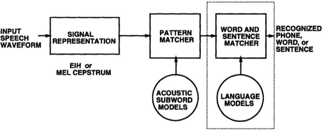
three main components - the signal representation module, the pattern matching module
and the word and sentence matching module - as illustrated in Figure 1-1 [24].
The first module, signal processing module, serves to extract information of interest from the large quantity of input speech data, in the form of a sequence of 'feature' vectors (not to be confused with the acoustic-phonetic features mentioned earlier). This parametric representation generally compresses speech while retaining relevant acoustic information such as location and energy of formants.
Speech is divided into smaller units (along time) called subword units, such as syllables, phones and diphones, for the purposes of recognition. In the 'training' phase, feature vectors
INPUT SPEECH WAVEFORI
Figure 1-1: Schematic of an automatic speech recognition system.
extracted from speech segments corresponding to a subword unit are clustered together and averaged using certain optimal algorithms to obtain a 'characteristic' unit model. A set of models is obtained for all subword units in this fashion. In the 'testing' phase, the second module, the pattern matcher, uses some distance measure to compare the input feature vectors representing a given unknown speech segment to the set of trained unit models. The choice of subword units affects recognition accuracy (e.g., dependent or context-independent models [25, 24]), as does the choice of distance measure (e.g., Euclidean,
log-likelihood [12]).
A list of top N candidates recognized for each given unit is passed to the third module,
the word and sentence level matcher. This module performs lexical, syntactic and semantic
analysis on candidate strings using a language model determined by the given recognition task, to yield a meaningful output. The third module is disconnected for the classification experiments conducted here, and the pattern matcher is modified to perform classification instead of recognition.
This study focuses on the choice of the signal representation module. Traditional spec-tral analysis schemes window the input speech at short intervals (10-20 milliseconds) and perform some kind of short-time Fourier transform analysis (STFT in chapter 6, [40]) to get a frequency distribution of the signal energy, preferably as a smooth spectral envelope. Two popular spectral analysis schemes are the filter bank model and the linear predictive coding (LPC) model (chapter 3 in [39]). The filter bank model estimates signal energy in uniformly or non-uniformly distributed frequency bands. LPC models the speech-sound production process, representing the vocal tract configuration which carries most of the speech related
information. The filter bank and LPC representations are often transformed to the cepstral
domain because cepstral coefficients show a high degree of statistical independence besides yielding a smoothened spectral envelope [29]. Cepstral analysis ([3]) is based on the theory of homomorphic systems (chapter 12 in [32]). Homomorphic systems obey a generalized principle of superposition; homomorphic analysis can be used to separate vocal tract and source information for speech signals [31]. A variation on cepstral analysis is the mel cep-strum, which filters speech with non-uniform filters on the mel frequency scale (based on
human perception of the frequency content of sounds). These spectral analysis schemes and others derived from them are primarily based on energy measurements along the frequency axis.
1.2 Recognition in Noise
The speech signal is affected differently by various environment-related adverse acoustic conditions such as reduced signal-to-noise ratio (SNR) in the presence of additive noise, signal cancellation effects in reverberation or nonlinear distortion through a microphone [18]. It is impractical to train for diverse (and often unknown) signal conditions, therefore it is advisable to make the ASR system more robust. Several techniques for improving ro-bustness have been proposed, including signal enhancement preprocessing [36, 7, 1], special
transducer arrangements [49], robust distance measures [47] and alternative speech
repre-sentations [28, 14, 45, 9]. Each of these techniques modifies different aspects of the ASR system shown in Figure 1-1.
In the case of distortion by additive noise, well-established speech enhancement tech-niques [27] can be used to suppress the noise. Such techtech-niques generally use some estimate of the noise such as noise power or SNR to obtain better spectral models of speech from noise-corrupted signals. In particular, in [36] and [7], the enhancement techniques have been directly applied to speech recognition. In [36], the optimal least squares estimator of
short-time spectral components is computed directly from the speech data rather than from an
assumed parametric distribution. Use of the optimal estimator increased the accuracy for a speaker-dependent connected digit recognition task using a 10 dB SNR database from 58% to 90%. This method, however, uses explicit information about the noise level, which the algorithm in [7] avoids. In [7], the short-time noise level as well as the short-time spectral
model of the clean speech are iteratively estimated to minimize the Itakura-Saito distortion
[15] between the noisy spectrum and a composite model spectrum. The composite model spectrum is a sum of the estimated clean all-pole spectrum and the estimated noise spec-trum. For a speaker-dependent isolated word (alphabets and digits) recognition task using 10 dB SNR test speech and clean training speech, the accuracy improved from 42% without preprocessing to 70% when both the clean training speech and the noisy testing speech were
preprocessed. The main limitation is the assumption of the composite model spectrum for
the noisy signal.
The work in [1] presents two methods for making the recognition system
microphone-independent, based on additive corrections in the cepstral domain. In the first,
SNR-dependent cepstral normalization (SDCN), a correction vector depending on the instan-taneous SNR is added to the cepstral vector. The second method, codeword-dependent
cepstral normalization (CDCN), computes a maximum likelihood (ML) estimate for both
the noise and spectral tilt and then a minimum mean squared error (MMSE) estimate
for the speech cepstrum. Cross-microphone evaluation was performed on an alphanumeric database in which utterances were recorded simultaneously using two different microphones
(with average SNR's of 25 dB and 12 dB). SDCN improved recognition accuracy from 19%-37% baseline to 67%-76%, and CDCN improved accuracy to 75%-74%. The main drawbacks of SDCN are that it requires microphone-specific training, and since normalization is based on long-term statistical models it cannot be used to model a non-stationary environment. CDCN does not require retraining for adaptation to new speakers, microphones or environ-ments.
In [49], several single-sensor and two-sensor configurations of speech transducers were evaluated for isolated-word recognition of speech corrupted by 95 dB and 115 dB sound pressure level (SPL) broad-band acoustic noise similar to that present in a fighter air-craft cockpit. The sensors used were an accelerometer, which is attached to the skin of the speaker and measures skin vibrations, and several pressure-gradient (noise-cancelling) microphones. Performance improvements were reported with various multisensor arrange-ments as compared to each single sensor alone, but the task was limited since the testing and training conditions were matched. Without adaptive training, there was no allowance for time-varying noise levels such as those caused by changing flying speed and altitude.
Robust distance measures aim to emphasize those regions of the spectrum that are less corrupted by noise. In [47], a weighted Itakura spectral distortion measure which weights
the spectral distortion more at the peaks than at the valleys of the spectrum is proposed.
The weights are adapted according to an estimate of the SNR (becoming essentially constant in the noise-free case). The measure is tested with a dynamic time warping (DTW) based speech recognizer on an isolated digit database for a speaker-independent speech recogni-tion task, using additive white Gaussian noise to simulate different SNR condirecogni-tions. This measure performed as well as the original unweighted Itakura distortion measure at high SNR's and significantly better at medium to low SNR's (at an SNR of 5 dB, this measure achieved a digit accuracy of 88% versus the original Itakura distortion which yielded 72%).
A technique for robust spectral representation of all-pole sequences, called the Short-Time Modified Coherence (SMC) representation, is proposed in [28]. The SMC is an all-pole modeling of the autocorrelation sequence of speech with a spectral shaper. The shaper, which is essentially a square root operator in the frequency domain, compensates
for the inherent spectral distortion introduced by the autocorrelation operation on the
sig-nal. Implementation of the SMC in a speaker-dependent isolated word recognizer showed its robustness to additive white noise. For 10 dB SNR spoken digit database, the SMC maintained an accuracy of 98%, while the traditional LPC all-pole spectrum representation fell from 99% accuracy in clean conditions to 40%.
Rasta (RelAtive SpecTrAl) [14] methodology suppresses constant or slowly-varying com-ponents in each frequency channel of the speech spectrum by high-pass filtering each channel with a filter that has a sharp spectral zero at zero frequency [14]. This technique can be used in the log-spectral domain to reduce the effect of convolutive factors arising from linear spectral distortions, or it can be used in the spectral domain to reduce the effect of additive stationary noise. For isolated digits, with training on clean speech and testing on speech corrupted by simulated convolutional noise, the Rasta-PLP (Perceptual Linear Predictive)
technique yielded 95% accuracy while LPC yielded 39% accuracy.
1.3 Motivation
While the energy based spectral analysis schemes such as LPC work well under similar
acoustic training and testing conditions, the system performance deteriorates significantly
under adverse signal conditions [4]. For example, for an alphanumeric recognition task, the performance of the SPHINX system falls from 77-85% accuracy with matched training and testing recording environments to 19-37% accuracy on cross conditions [1]. Robustness im-proving techniques explicitly based on matched training and testing conditions, noise level, SNR or the particular signal distortion, such as those described in Section 1.2, are clearly
not desirable for robustness to multiple adverse acoustic conditions. The human auditory
system seems to exhibit better robustness than any machine processor under different
ad-verse acoustic conditions; it is successful in correctly perceiving speech in a wide range of
noise levels and under many kinds of spectral distortions.
For robust speech recognition, speech processing models based on the human auditory system have been proposed, such as the representation in [45]. In this model, first-stage spectral analysis is performed with a bank of critical-band filters, followed by a model of
nonlinear transduction in the cochlea that accounts for observed auditory features such as
adaptation and forward masking [46, 13]. The output is delivered to two parallel chan-nels, one of them yields an overall energy measure equivalent to the average rate of neural discharge, called the mean rate response, the other is a synchrony response which yields enhanced spectral contrast showing spectral prominences for formants, fricatives and stops. This auditory model has yielded good results for isolated word recognition [16, 26].
The EIH is another speech representation motivated by properties of the auditory system
[9]. It employs a coherence measure as opposed to the direct energy measurement used in conventional spectral analysis. It is effectively a measure of the spatial (tonotopic) extent of
coherent neural activity across a simulated auditory nerve. The EIH is computed in three
stages - bandpass filtering of speech to simulate basilar membrane response, processing of the output of each filter by level-crossing detectors to simulate inner hair cell firings, and
the accumulation of an ensemble histogram as a heuristic for information extracted by the
central nervous system.
An evaluation of the EIH [9] was performed with a DTW based recognizer on a 39-word alpha-digit speaker-dependent task in the presence of additive white noise. In high SNR the EIH performed similarly to the DFT front end whereas at low SNR it outperformed the DFT front end markedly. Another study [16] involved the comparison of mel cepstrum
and three auditory models - Seneff's mean rate response and synchrony response [44], and
the EIH. It was performed on a speaker-dependent, isolated word task (TI-105 database) using continuous density Hidden Markov Models (HMMs) with Gaussian state densities. On the average, the auditory models gave a slightly better performance than mel cepstrum for training on clean speech and testing on speech distorted by additive noise or spectral
variability (e.g., soft or loud speech, telephone model, recording environment model, head shadow).
This study differs from the previous evaluations in six ways: it uses a continuous speech
database instead of isolated or connected word databases, the size of the database is much
larger than those used earlier (4380 sentences as compared to the 39-word and 105-word vocabularies), phone classification is performed instead of word recognition, mixture
Gaus-sian HMMs are used in contrast to the DTW based recognizer or the GausGaus-sian HMMs used
in previous experiments, static, and static and dynamic features are evaluated separately,
and in addition to the average results, a breakdown of the average results into results for different phonetic groups is provided along with a qualitative analysis of confusion matrices of these groups.
The two speech representations, mel cepstrum and EIH, are implemented as front ends to a state-of-the-art continuous speech ASR and evaluated under different conditions of distortion on the TIMIT database (male speakers). The TIMIT is used because it is a standard, phonetically rich, hand segmented database. The recognizer is first trained on clean speech and then tested under three acoustic conditions - clean speech, speech through a telephone channel and speech under room reverberations (the last two conditions are simulated; training speech is also evaluated).
Evaluation is based on phone classification, where the left and right phone boundaries
are assumed fixed and only the identity of the phone is to be established. Classification is performed, instead of recognition (which assumes no such prior information about the input speech), to focus on the front end and eliminate issues like grammar, phone insertion and phone deletion that are involved in the recognition process. The objective here is to
observe the effects of signal distortion on the signal representation and statistical modeling.
The performance is displayed as average percent of phones correctly classified, and in the form of confusion matrices to provide diagnostic information. Classification experiments are conducted for (1) different sets of feature vectors, with and without time-derivatives, to observe the relative contribution of dynamic information and for (2) different iterations of automatic resegmentation of the database, which provides boundaries that are consistent with a well-defined objective measure, and is used in most current ASR systems.
The organization of the thesis is as follows:
1. Chapter 2 sketches the process of sound production, and contains a short description of different sound classes, which should serve to give some background for the discussion
of results in Chapter 5. The classification system used in this work is based on
an HMM recognition framework; a brief outline of Hidden Markov Models is also included.
2. Chapter 3 describes the two signal representations, mel cepstrum and Ensemble In-terval Histogram, evaluated in this study. A brief description of part of the human auditory mechanism is given as background for EIH. The details of implementation for both representations are provided. The method of calculation of dynamic features
is described.
3. Chapter 4 contains a description of the experimental framework. The training and testing subsets used from the TIMIT database are described, along with the set of phones used for classification. The phone classification system and the distortion
conditions - telephone channel and room reverberation simulations - are described.
4. Chapter 5 lists the results obtained for different classification experiments, with static
features and static and dynamic features, and with automatically resegmented phone
boundaries. The average classification results are discussed, and broad trends in the
confusion matrices are observed.
5. Chapter 6 summarizes the work done in this thesis and the conclusions drawn from
the results. Possible directions for future research are provided.
1.4 Summary
This chapter introduced the problem of automatic speech recognition and some of the
issues in current speech research. The problem of recognizing noisy speech and different
approaches taken to attain robustness in speech recognition were described. The next
chapter contains a brief description of Hidden Markov Models and speech sounds, that
Chapter 2
Background
Speech is composed of a sequence of sounds carrying symbolic information in the nature,
number and arrangement of these sounds. Phonetics is the study of the manner of sound
production in the vocal tract and the physical properties of the sounds thus produced. This
chapter contains an outline of the physiology of sound production in Section 2.1.1 and a brief description of the different sounds in American English classified by the manner of production in Section 2.1.2. The references are drawn mainly from Chapter 3 in [40] and Chapters 4 and 5 in [30]. A brief description of Hidden Markov Models (HMM's) is provided in Section 2.2. Further reading on HMM techniques can be found in [38].
2.1 Speech Production and Speech Sounds
2.1.1
Speech Production
The message to be conveyed via spoken sounds is formulated in the brain and then
uttered aloud with the execution of a series of neuromuscular commands. Air is exhaled from the lungs with sufficient force, accompanied by a vibration of the vocal cords (or vocal
folds) at appropriate times, and finally shaped by motion of the articulators - the lips, jaw,
tongue, and velum. Figure 2-1 is a sketch of the mid-sagittal cross-section of the human vocal apparatus [39]. The vocal tract begins at the opening between the vocal cords called
the glottis, and ends at the lips. It consists of two parts, the pharynx (the section between
the esophagus and the mouth) and the oral cavity or the mouth. The nasal tract is the
cavity between the velum and the nostrils.
Depending on the pressure gradient across the glottis, the mass and tension of vocal folds, two kinds of air flow are generated upwards through the pharynx, quasi-periodic and noise-like. Quasi-periodic (harmonically related frequencies) pulses of air are produced when the vocal folds vibrate in a relaxation oscillation at a fundamental frequency. These excite the resonant cavities in the vocal tract resulting in voiced sounds like vowels.
Broad-spectrum (wide range of unrelated frequencies) noise-like air flow is generated by forcing air at a high enough velocity through a constriction in the vocal tract (while the vocal cords are relaxed), so as to cause turbulence. This produces unvoiced sounds like /s/ (as spoken in sad), /f/ (fit) by exciting the vocal tract with a noise-like waveform, and plosive sounds like /b/ (big), /p/ (pig) when air pressure is built up behind a complete closure in the oral
cavity and then abruptly released.
/
ARTICULATORS
DIAPHI
Figure 2-1: Cross section of the speech-producing mechanism
The vocal tract is a tube with a non-uniform and variable cross-sectional area. The nasal tract remains disconnected from the vocal tract for most sounds and gets acoustically coupled to it when the velum is lowered to produce nasal sounds. The resonant frequencies of the vocal tract are called formants; they depend on its dimensions in a manner similar to the resonances in wind instruments. Different sounds are formed by varying the shape of the tract to change its frequency selectivity. The rate of change of vocal tract
con-figuration categorizes sounds as continuant and noncontinuant. The former are produced when a non time-varying vocal tract configuration is appropriately excited, for e.g., vowels
and nasals (/m/ in mild) , and the latter are produced by a time-varying vocal tract, for
e.g., stop consonants (/d/ in dip) and liquids (/1/ in lip). Vowels, which are continuant sounds, can be differentiated into close, open, high, low and rounded based on the positions of the articulators. The consonants can also be alternatively classified by their
place-of-articulation, for e.g., labial (lips), alveolar (gums), velar (velum), dental, palatal or glottal,
along with the manner-of-articulation (plosive, fricative, nasals etc.). There are different ways of characterizing sounds based on the physical mechanism of production.
2.1.2
Speech Sounds
PHONEMES in American English
Vowels Consonants Semivowels Diphthongs
Front Mid Back
iy (eat) er (bird) uw(boot)
ih (it) ah (but) uh (foot)
eh (pet) ax (about) ow (boat)
ae (at) ao (baud) . aa (father) . . ay (sky) oy (toy) aw (wow) ey (wait) Liquids Glides r (red) w (wet) I (let) y (yes) . ...
--Fricatives Nasals wnisper Anrcaes Stops
m (mom) h (had) jh (ar) /
n (nun) ch (char)
ng (sing) /
Voiced Unvoiced Voiced Unvoiced
v (van) f (fit) b (big) p (pop)
dh (this) th (thin) d (dig) t (tip)
z (zoo) s (sit) g (get) k (kit)
zh (measure) sh (she)
Figure 2-2: Phonemes in spoken American English
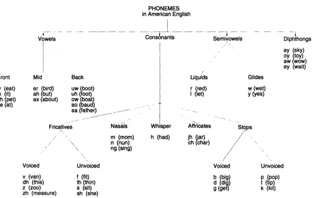
For the purposes of speech recognition, speech is segmented into subword units called
phones, which are the acoustic realizations of abstract linguistic units called phonemes.
Phonemes are the sound segments that carry meaning distinctions, identified by minimal pairs of words that differ only in part ([30]). For example, fat and cat are different sounding words that have different meanings. They differ from each other only in the corresponding first sounds /f/ and /c/, which makes /f/ and /c/ phonemes. Figure 2-2 shows the set of phonemes in spoken American English. The figure is based on the categorization in Chapter
4 in [30].
Vowels are produced by an essentially time-invariant vocal tract configuration excited by quasi-periodic air pulses, and are the most stable set of sounds. They are generally longer in duration than consonants, and are spectrally well-defined. All vowels are voiced sounds.
Different vowels can be characterized by their first, second and/or third formants, which are determined by the area function - the dependence of the area on the distance along the vocal tract. The area function depends mainly on the tongue hump, which is the mass of the tongue at its narrowest point. Vowels can be classified by either the tongue hump position as front, mid, back vowels (shown in Figure 2-2), or by the tongue hump height as high, mid, low vowels. The vowel formant space is illustrated in Figure 2-3 based on formant values taken from Chapter 4 in [30]. The vowels are divided into different categories used later in Chapter 5, front, central and back, and high, mid and low.
Zuu- 300-HIGH F 400-1 500 n MID H z 600 700-LOW ann-2400 2200 2000 1800 1660 1400 1200 1000 800
FRONT CENTRAL BACK
F2 (hertz)
Figure 2-3: The vowel formant space 2. Diphthongs
Diphthongs are described as combinations of certain 'pure' vowels with a second sound and are voiced. Figure 2-2 shows four diphthongs /ay/,/oy/, /aw/, /ey/.
According to Chapter 3 of [40], a diphthong is defined as a gliding monosyllabic speech
item that starts at or near the articulatory position for one vowel and moves to or
toward the position for another. It is produced by smoothly varying the vocal tract configuration from that for the first vowel to the configuration for the second vowel. In Chapter 5 in [30], diphthongs are described as combinations of vowels and glides
(glides are described after the liquids, which come next). /ay/, /ey/ and /oy/ are
)1' iy(eat) : ( uw(boo ih(it) ... ... u h (foo t) ... er(bird) eh(pet) ow(boat) ah(but) ... . ... ... K .ao(baud). ... .ao(baud). ae(at) : aa(father) A I I I I I I
combinations of the corresponding vowels and the glide /y/. /aw/ is a vowel followed by the glide /w/, as /ow/ sometimes is (the diphthong /ow/ in mow, as opposed to the vowel /ow/ in boat).
3. Liquids
Liquids and glides are sometimes described as semivowels. Both are gliding transitions in vocal tract configuration between the adjacent phonemes. They consist of brief vowel-like segments and are voiced sounds, but their overall acoustic characteristics depend strongly on the context (neighboring phonemes).
The liquids are /r/ and /1/. /r/ has low values for all first three formants, and is the only phoneme in American English that has a third formant below 2000 Hz. /1/ shows a slight discontinuity at vowel junctures, and is the only English lateral consonant (created by allowing air to pass on either side of the tongue). Both phonemes have an alveolar place-of-articulation.
4. Glides
The glides are /w/ and /y/, and are voiced sounds. They are always followed by vowels, and have a labial and alveolar place-of-articulation respectively. They do not
exhibit formant discontinuities at vowel junctures.
5. NasalsThe nasal sounds /m/, /n/ and /ng/ are produced by lowering the velum to
acousti-cally couple the nasal tract to the vocal tract, with glottal excitation and a complete
constriction of the vocal tract at some point in the oral cavity. Sound is radiated
through the nostrils in this case and the mouth acts as a resonant cavity. The
res-onances of the spoken nasal consonants and nasalized vowels are spectrally broader (more damped) than those of vowels.
The total constriction made in the vocal tract is different for the three nasals: /m/ is a labial, /n/ an alveolar and /ng/ is a velar sound. The closures for these three sounds are made in the same place as the corresponding stops. Both kinds of sounds are produced with complete closure of the oral cavity, the difference is in the aperture of the velic port. For nasals, air is released through the nose and since there is no pressure buildup, no burst occurs when the oral closure is released.
All three nasals have a prominent low frequency first formant, called the nasal formant. There are clear and marked discontinuities between the formants of nasals and those of adjacent sounds.
6. Fricatives
Fricatives are characterized by the frictional passage of air flow through a constriction
at some point in the vocal tract. The steady air stream used to excite the vocal tract
becomes turbulent near the constriction. The back cavity below the constriction traps
energy like the oral cavity in the case of nasals and introduces anti-resonances in the sound radiated from the lips.
There are two kind of fricatives, voiced and unvoiced. /v/, /dh/, /z/, /zh/ are voiced and /f/, /th/, /s/, /sh/ are unvoiced. The sounds in the two sets correspond exactly in terms of places-of-articulation, which are labio-dental, dental, alveolar and palatal respectively.
Out of the unvoiced fricatives, /th/ and /f/ have little energy, whereas /s/ and /sh/
have a considerable amount. All the unvoiced fricatives except /f/ show no energy below 1200 Hz. The voiced fricatives show energy in the very low frequency range, referred to as the voice bar.
7. Stops
Stops (or stop consonants) are noncontinuant, plosive sounds. There are two kinds of stops, /b/, /d/, /g/ are voiced and /p/, /t/, /k/ are unvoiced. These also corre-spond in their places-of-articulation, which for both sets are labial, alveolar and velar respectively.
No sound is radiated from the mouth during the time of total constriction of the vocal tract; this time interval is called the 'stop gap'. However, in the case of voiced stops, some low frequency energy is often radiated through the walls of the throat when the vocal cords can vibrate in spite of a total constriction in the tract. The distinctive characteristic of stops visible in a spectrogram is the presence of two distinct time segments, the closure and the burst. If the stop is followed by a voiced sound, the interval after the burst and before the sound is called the voice onset time (VOT).
In the case of unvoiced stop consonants, after the stop gap, there is a brief period
of friction followed by an interval of aspiration before voiced excitation begins. The duration and frequency content of the frication noise and aspiration vary with the unvoiced stop.
Stops are noncontinuants, generally of short duration, and are more difficult to identify from the spectral information alone. Their properties are greatly influenced by the context.
8. Affricates
An affricate consists of a stop and its immediately following release through the ar-ticulatory position for a continuant nonsyllabic consonant. The English affricates are /ch/ and /jh/, /ch/ is a concatenation of the stop /t/ and the unvoiced fricative /sh/. Similarly /jh/ is a combination of the voiced stop /d/ and the voiced fricative /zh/. The two affricates function as a single unit but their spectral properties are like other stop-fricative combinations.
Affricates also display a closure-burst in the spectrogram, followed by the fricative region.
9. Whisper sounds
The phoneme /h/ is produced by exciting the vocal tract with a steady air flow
without vibration of the vocal cords. Turbulence is produced at the glottis. This is
also the mode of excitation for whispered speech. The spectral characteristics of /h/ depend on the vowel following /h/ because the vocal tract assumes the position for
the following vowel during the production of /h/.
2.2 Hidden Markov Models
The two speech representation, mel cepstrum and EIH, are described in Chapter 3. It is shown how a speech utterance, consisting of periodic measurement samples of the acoustic waveform, can be converted into a sequence of observation vectors, each of which corresponds to a fixed-length window or frame of N speech samples. The sequence of feature vectors, called a template, can therefore serve as a model of the speech utterance. However, different templates obtained from the same person speaking at different times are not identical. Clearly, there is even more variation across different speakers. One way to capture this variability is to model speech as a stochastic sequence.
A commonly used stochastic framework used in speech recognition is hidden Markov modeling (HMM). An overview of Hidden Markov Models can be found in [38]. HMMs
are stochastic models of the speech signal designed to represent the short time spectral
properties of sounds and their evolution over time, in a probabilistic manner. An HMM
as used in speech recognition is a network of states connected by transitions. Each state represents the hidden probability distribution for a symbol from finite set of alphabets, such as a phone from a list of allowed phones. This output probability density function is used to
determine the observation sequence by maximum likelihood estimation, using the transition
probabilities associated with going from one state to the next.
Three key problems of HMMs are [38]:
1.
Given the observation sequence0
= 0102 ... OT, and a modelA,
what is the efficient way to find P(OA), the probability of the observation sequence given a model ? Thisis referred to as the scoring problem, i.e., given a model, compute the likelihood score of an observation. This is a measure of how well the utterance matches the model. 2. Given the observation sequence and the model, how should a state sequence Q =
q1q2 ... qT which is optimal in some meaningful sense be chosen ? This is referred to
as the segmentation problem, because each vector Oi in the sequence is assigned to a state. For left-to-right models, since each transition can only be to the same state or the next state, this is equivalent to dividing the observation sequence into N segments, each corresponding to a state. That is, a set of transition times rl, T2,..., rN, are
obtained so that the vectors Oj, where ri
<j < ri+l are assigned to state Si.
P(OIA)? This is called the training problem, encountered when a maximum like-lihood model for a word, syllable, etc. must be built from some training utterances. The solutions of these problems are detailed in [38] and further references contained therein. A brief description of the solutions to each of the problems is given next.
The objective of training is to find a A so as to maximize the likelihood of P(O[A). The absolute maximum is difficult to find, and only iterative algorithms like the estimate-maximize (EM) algorithms can be used to find locally maximum solutions. A widely known
training algorithm of this type is the Baum-Welch reestimation algorithm [34].
The actual training procedure used in experiments here is also an EM algorithm, called the segmental k-means training algorithm [41]. It trains a subword model out of several utterances of the same subword through the following steps:
1. Initialization: Each speech utterance, represented by a sequence of feature vectors, is uniformly segmented into states i.e. each state in a subword initially has roughly the same number of feature vectors assigned to it. The TIMIT hand segmentation is
used to obtain phone boundaries.
2. Estimation: Using the data thus segmented, the parameters of each state are esti-mated. The feature vectors in each state are clustered into different mixture compo-nents using a K-means algorithm. The mean vectors, the variance vectors and the mixture weights are estimated for each cluster. The sample mean and covariance of the vectors in each cluster are used as maximum likelihood estimates of the mean vector and covariance matrix of each mixture component in the state. The weight of each mixture component is estimated based on the proportion of vectors in each cluster. This gives a first set of HMMs for all the states of all subword units.
3. Segmentation:
The HMM thus estimated is used to resegment the training data into new units with
Viterbi decoding.
4. Iteration: Steps 2 and 3 are repeated until convergence.
The acoustic space can be modeled by a finite number of distinguishable spectral shapes, which correspond to the states of an HMM. Alternatively, the speech signal can be viewed as being composed of quasi-stationary segments produced by stable configurations in the
articulatory structures, connected by transitional segments produced during the time the
articulatory structures evolve from one stable configuration to another. Each state of an HMM can thus either represent a quasistationary segment in the speech signal or a transi-tional segment. More generally, each state of an HMM can be used to model some salient features of sound so that it can be distinguished from other neighboring states.
In addition, HMMs can be hierarchical, such that each state or node can be recursively expanded into another HMM. Thus at the highest level, there can be a network of words, where each word is represented by a state in the HMM. Each word can expand into an HMM,
whose states each represent a particular phone. Each of these word states can further be
expanded into an HMM whose states each represent some acoustic sound or phone model.
2.3 Summary
This chapter outlined the speech production process, and described some characteristics
of sounds classified by the manner of production. An outline of the Hidden Markov Modeling (HMM) procedure was also provided. The next chapter discusses the two feature extraction
Chapter 3
Signal Representations- Mel
Cepstrum and Ensemble Interval
Histogram
The two signal representations evaluated in this thesis are described in this chapter. The mel cepstrum (MEL) representation is based on Fourier analysis, and the Ensemble Interval Histogram (EIH) is based on auditory modeling. A brief introduction to the theoretical basis for both front ends is provided, followed by a description of the computational procedures. A short comparison of the two front ends is given at the end.
3.1 Mel Cepstrum
3.1.1
Mel Scale
Psychophysical studies have shown that human perception of the frequency content of sounds, for either pure tones or speech signals, does not correspond to a linear scale. The human ear is more sensitive to lower frequencies than the higher ones [48]. For each tone with a certain actual frequency in hertz, a subjective pitch is measured on the 'mel' scale. The pitch of a 1 kHz tone at 40 dB higher than the perceptual hearing threshold is defined as 1000 mels. The subjective pitch is essentially linear with the logarithmic frequency above
1000 Hz.
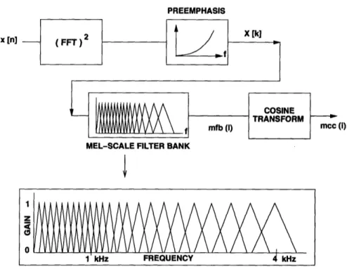
MEL accounts for this frequency sensitivity by first filtering speech with a filterbank which consists of filters that have increasing bandwidth and center-frequency spacing with increasing frequency [5].