Spatial Issues in Modeling LoRaWAN Capacity

(1)

HAL Id: hal-02378078

https://hal.archives-ouvertes.fr/hal-02378078

Submitted on 24 Nov 2019

HAL is a multi-disciplinary open access

archive for the deposit and dissemination of

sci-entific research documents, whether they are

pub-lished or not. The documents may come from

teaching and research institutions in France or

abroad, or from public or private research centers.

L’archive ouverte pluridisciplinaire HAL, est

destinée au dépôt et à la diffusion de documents

scientifiques de niveau recherche, publiés ou non,

émanant des établissements d’enseignement et de

recherche français ou étrangers, des laboratoires

publics ou privés.

Spatial Issues in Modeling LoRaWAN Capacity

Andrzej Duda, Martin Heusse

To cite this version:

Andrzej Duda, Martin Heusse.

Spatial Issues in Modeling LoRaWAN Capacity.

Proceedings

of the 22Nd International ACM Conference on Modeling, Analysis and Simulation of

Wire-less and Mobile Systems, Nov 2019, Miami Beach, FL, USA, Unknown Region.

pp.191–198,

(2)

Spatial Issues in Modeling LoRaWAN Capacity

Andrzej Duda

andrzej.duda@imag.fr

Univ. Grenoble Alpes, CNRS, Grenoble INP, LIG Grenoble, France

Martin Heusse

martin.heusse@imag.fr

Univ. Grenoble Alpes, CNRS, Grenoble INP, LIG Grenoble, France

ABSTRACT

All existing models for analyzing the performance of LoRaWAN assume a constant density of nodes within the gateway range. We claim that such a situation is highly unlikely for LoRaWAN cells whose range can attain several kilometers in real-world deploy-ments. We thus propose to analyze the LoRa performance under a more realistic assumption: the density of nodes decreases with the inverse square of the distance to the gateway.

We use the LoRaWAN capacity model by Georgiou and Raza to find the Packet Delivery Ratio (PDR) for an inhomogeneous spatial distribution of devices around a gateway and obtain the number of devices that benefit from a given level of PDR. We analyze the Lo-RaWAN capacity in terms of PDR for various spatial configurations and Spreading Factor allocations.

CCS CONCEPTS

• Networks → Network performance modeling; Very long-range networks; Sensor networks.

KEYWORDS

LoRaWAN; Packet Delivery Ratio; capacity; modeling; inhomoge-neous density

ACM Reference Format:

Andrzej Duda and Martin Heusse. 2019. Spatial Issues in Modeling Lo-RaWAN Capacity. In 22nd Int’l ACM Conference on Modeling, Analysis and Simulation of Wireless and Mobile Systems (MSWiM ’19), November

25–29, 2019, Miami Beach, FL, USA.ACM, New York, NY, USA, 8 pages.

https://doi.org/10.1145/3345768.3355932

1 INTRODUCTION

LoRa [1] is a recent example of a Low Power Wide Area Network (LPWAN) that can provide wireless connectivity to a large number of IoT devices over long distances. It defines a physical layer based on the Chirp Spread Spectrum (CSS) modulation [2] and a simple channel access method similar to ALOHA called LoRaWAN [3]. The LoRa CSS modulation results in good sensitivity enabling transmis-sions over long distances: a range of several kilometers outdoors and hundreds of meters indoors.

A LoRa end device can vary several transmission parameters: channel bandwidth (BW), transmission power (TP), coding rate

Permission to make digital or hard copies of all or part of this work for personal or classroom use is granted without fee provided that copies are not made or distributed for profit or commercial advantage and that copies bear this notice and the full citation on the first page. Copyrights for components of this work owned by others than ACM must be honored. Abstracting with credit is permitted. To copy otherwise, or republish, to post on servers or to redistribute to lists, requires prior specific permission and/or a fee. Request permissions from permissions@acm.org.

(CR), and spreading factor (SF). The achievable data rates depend on some of the parameters: a higher bit rate results from lower SF (at the cost of a shorter range), higher BW, and CR of 4/5. The bit rates range from 293 b/s to 11 kb/s, the low bit rate resulting in long transmission times: 2.466 s for sending 59 B at SF12.

In addition to the physical layer parameters, the LoRa perfor-mance in terms of the Packet Delivery Ratio (PDR) and scalability to a large number of devices strongly depend on the LoRaWAN access method similar to unslotted ALOHA: a device may wake up at any instant and start transmitting a packet without testing for on-going transmissions.

The previous analytical studies investigated LoRa performance for an increasing number of nodes around a gateway with an impor-tant assumption: the density of nodes within the gateway range is uniform [4–9]. However, such an assumption is not realistic for cells covering large areas of several square kilometers for two reasons. First, measurement studies in cellular networks showed that spatial traffic distribution is highly non-uniform across different cells [10–14] with complex patterns that include hot spots with a high density and other less dense places. For instance, Lee et al. [11] demonstrated based on traffic measurements that the spa-tial distribution of the traffic density across different cells can be approximated by the log-normal or Weibull distributions depend-ing on time and space. As cells in cellular networks can be smaller than LPWANs (target range of several kilometers), we expect that spatial traffic distribution in LoRa networks will also be highly non-uniform. We can also consider that the distribution of devices follows in fact the same pattern as we can usually observe for pop-ulation and building densities in cities: apart from the saturated downtown, the density decreases with the distance from the center— it is much higher downtown than in suburbs. The deployment of gateways by LPWAN operators will probably also follow the same strategy as in cellular networks—place networks close to potential users and create hot spots near high density areas.

Second, there is a discouraging effect when placing a device far from the gateway in a LoRaWAN cell: the device needs to use large SF (e.g., SF11 or SF12) to get its transmissions through, which means long transmission times, so increased contention (more collisions) and higher energy consumption. For instance, a device using SF11 will roughly consume 10 times more energy for a transmission than when using SF7. Moreover, if we consider an equidistant dis-tribution of spreading factors, which is the most popular spatial model adopted in the analyses with concentric annuli spaced at 1 km intervals, there are more devices with larger SF such as SF11 and SF12 than devices in the area of SF7. There are also no devices outside the zone of SF12, a kind of a disruptive irregularity difficult to observe in real world deployments.

We claim that uniform node density is highly unlikely for large cells so we propose to analyze LoRa performance under a more

(3)

realistic assumption: the density of nodes decreases with the inverse

square of the distanceto the gateway. The inverse-square law is

common in physics stating that a specified physical quantity or intensity is inversely proportional to the square of the distance from the source of that physical quantity. For instance, radio wave transmission in free space follows an inverse square law for power density. We consider that such a spatial model corresponds better to real-world LoRaWAN deployments than the models based on the constant density.

In this paper, we use the model by Georgiou and Raza [4] to find the Packet Delivery Ratio (PDR) for inhomogeneous spatial distributions of devices around a gateway and obtain the number of devices that benefit from a given level of PDR. Unlike Georgiou and Raza, we adopt a realistic assumption about generated traffic: nodes send packets at the smallest possible time interval determined by the largest duty cycle possible at SF12. Under this assumption, devices generate packets in a way defined by a sensing application unlike the model by Georgiou and Raza that assumes 1% duty cycle of all devices regardless of SF, which means that a device that changes from SF8 to SF7 starts sending packets twice more often. We also modify the model expression for traffic intensity so it correctly reflects the unslotted ALOHA behavior (instead if slotted ALOHA). In the rest of the paper, we describe the basics of LoRa networks (Section 2) and present the PDR model (Section 3). In Section 4, we analyze LoRaWAN capacity in terms of PDR for different spatial configurations. Finally, we discuss related work (Section 5) and draw some conclusions (Section 6).

2 LORAWAN BASICS

We briefly recall the basic characteristics of LoRaWAN.

Devices can control the physical layer of LoRaWAN through the following parameters [15]:

•Bandwidth (BW): it is the range of transmission frequencies.

We can configure the bandwidth between 7.8 kHz and 500 kHz. A larger bandwidth allows for a higher data rate, but results in lower sensitivity.

•Spreading Factor (SF) characterizes the number of bits

car-ried by a chirp: SF bits are mapped to one of N = 2SF_possible

frequency shifts in a chirp. SF varies between 6 (7 in practice) and 12, with SF12 resulting in the best sensitivity and range, at the cost of achieving the lowest data rate and worst energy consumption. Decreasing the SF by 1 unit roughly doubles the transmission rate and divides by 2 the transmission du-ration as well as energy consumption.

•Coding Rate (CR): it corresponds to the rate of Forward

Error Correction (FEC) applied to improve packet error rate in presence of noise and interference. A lower coding rate results in better robustness, but increases the transmission time and energy consumption. The possible values are: 4/5, 4/6, 4/7, and 4/8.

•Transmitted Power (TP): LoRaWAN defines the following

values of TP for the EU 863-870 MHz band: 2 dBm, 5 dBm, 8 dBm, 11 dBm, and 14 dBm.

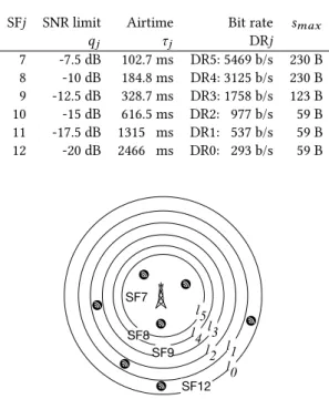
Table 1 presents SFj, data rate DRj, Signal-to-Noise Ratio (SNR)

limit, airtime τj, and smax, the maximum payload size. τjdenotes

Table 1: LoRa parameters for BW of 125 kHz.

SFj SNR limit Airtime Bit rate smax

qj τj DRj 7 -7.5 dB 102.7 ms DR5: 5469 b/s 230 B 8 -10 dB 184.8 ms DR4: 3125 b/s 230 B 9 -12.5 dB 328.7 ms DR3: 1758 b/s 123 B 10 -15 dB 616.5 ms DR2: 977 b/s 59 B 11 -17.5 dB 1315 ms DR1: 537 b/s 59 B 12 -20 dB 2466 ms DR0: 293 b/s 59 B

How Many Sensor Nodes Fit In A LoRAWAN Cell?

Author 1

⇤

_{, Author 2}

†

_{, Author 3}

⇤ ⇤

_{Affiliation 1}

†

_{Affiliation 2}

Abstract—We propose a model to estimate the number of nodes

that a LoRaWAN cell can handle, when they all have the same

traffic generation process. The model predicts the packet delivery

ratio for any cell range and node density. Moreover, we find that

the considered traffic gives prominence to the problem of suitable

allocation of spreading factors (SF), which consists in setting SF

boundaries to balance between attenuation and collisions. When

using several repetitions for each data packet, the number of

nodes is in the order of a couple thousands in the case of a short

range cell; it drops to several hundreds when more distant nodes

need to switch to higher spreading factors, which increases the

level of contention.

I. I

NTRODUCTION

LoRaWAN is a Low Power Wide Area Network technology

widely used to build nation-wide cellular networks as well as

private IoT data collection systems. The physical layer uses

CSS (Chirp Spread Spectrum) for robust communication in

the sub-GHz ISM band. There are several spreading factors

(SF) to choose from, which allows to trade data rate for range.

LoRaWAN defines a channel access method based on ALOHA

with rare feedback from the gateway. Transmissions using

different spreading factors are quasi-orthogonal—in case of

a collision, both frames succeed if they are not significantly

stronger from each other. In the same SF, a frame succeeds if

it is significantly stronger than the other.

While the radio channel capacity of LoRaWAN is already

well investigated [1]–[6], we tackle this problem from a

slightly different perspective. We seek to assess the number

of nodes with a similar traffic load that a single gateway

can handle before the packet delivery ratio (PDR) drops to

unacceptable levels. In this paper, we bring the following three

contributions:

1) A simple model for collisions and physical capture,

which gives better insight into the dynamics of packet

loss due to ALOHA with physical capture.

2) A traffic model where all nodes have the same traffic

intensity, in which case it is relevant to express the cell

capacity in terms of number of nodes. This assumption is

the most realistic, since traffic generation is determined

by the application, for example periodic sensing or

metering, regardless of the distance to the gateway.

3) An SF allocation to improve and even out the PDR

throughout the cell. We optimize the SF boundaries to

balance the opposite effects of attenuation and collisions.

These two last factors are antagonistic because switching to a

larger SF results in more robust transmissions but with longer

duration, which increases contention. We will see that it is wise

to control the number of nodes using higher SFs because they

Table I: Notations

Spatial density of nodes ⇢

Traffic generation intensity t

Frame transmission duration at Data Rate DRj ⌧j

Distance of farthest node using DRj lj

Traffic occupancy (in Erlang) at DRj vj

Average channel gain at distance d g(d)

SNR threshold for DRj qj

Transmission power, in-band noise power P, N

Success probability, due to attenuation, fading, thermal noise H

Success probability, due to collisions Q

−10 −5 0 5 10 − 10 − 5 0 5 10 rep(0, 6) rep(0, 6) SF7 SF8 SF12 SF9 l5 l4l3 l2 l1 l0

Figure 1: Annuli of SF allocation around the gateway

occupy much more channel capacity than nodes with lower

SFs. Conversely, for a lower node density, channel usage may

be low for e.g. SF7, since few nodes are able to take advantage

of it.

II. PDR

IN A

L

O

R

A

WAN

CELL FOR HOMOGENEOUS TRAFFIC

In a LoRaWAN cell, a frame may be lost for two reasons

(and maybe both): i) the SNR is below the reception threshold

or ii) a collision occurs and the signal is not strong enough

relatively to the interference.

We restrict our analysis to the basic LoRa CSS modulations

with BW of 125 kHz and SF in 12, 11,. . . 7, which corresponds

to data rates DRj, with j = 0, 1, . . . 5, and SF = 12

j.

A. Channel model

We use the Okumura-Hata model for path loss attenuation

(also used by Bankov [7] and Magrin [8]), using the suburban

environment variant with an antenna height of 15 m. This

empirical model is slightly less favorable than adopting an

arbitrary path loss exponent as in most of the previous work

we cite. We have chosen the Okumura-Hata model because it

is more realistic, but the results are qualitatively similar. We

consider a GW-side antenna gain of 6 dB which compensates

for a receiver noise factor of 6 dB.

Page 1 of 9

IEEE Communications Letters

1

2

3

4

5

6

7

8

9

10

11

12

13

14

15

16

17

18

19

20

21

22

23

24

25

26

27

28

29

30

31

32

33

34

35

36

37

38

39

40

41

42

43

44

45

46

47

48

49

50

51

52

53

54

55

56

57

58

59

60

Figure 1: Annuli of SF configurations around a gateway

the transmission duration of the maximum size frame at data rate DRj.

LoRaWAN defines an access method similar to ALOHA: a device wakes up at any instant and sends a packet right away. It then wakes up after a delay to receive a downlink frame, if the transmitted frame was of the Confirmed Data type. Collisions occur when two devices transmit packets at the same time. However, unlike in the pure ALOHA scheme, a receiver can correctly receive a frame in presence of interfering signals, because the LoRa physical layer is robust enough to resist significant interference. The capture effect has important impact on LoRa performance. Taking into account the capture effect, Haxhibeqiri et al. [16] showed that when the number devices increases to 1000 per gateway, the packet loss rate only increases to 32%, which is low compared to 90% in pure ALOHA for the same load.

In the following sections, we assume LoRa modulations with 125 kHz bandwidth and spreading factors SF{12 − j} that result in data rates DRj, with j = 0, 1, . . . 5 (see Table 1).

3 MODEL FOR SUCCESSFUL PACKET

DELIVERY

We consider a LoRaWAN cell in which devices choose SF (so the data rate) based on the distance to the gateway, which corresponds

to the annuli view presented in Figure 1. ljdenotes the distance to

the farthest device that uses SF{12 − j} so its data rate is DRj. l0is

the maximum transmission range.

We assume that devices are located at random in the annulus

at ljaccording to a Poisson Point Process (PPP) with intensity ρj.

(4)

Table 2: Equidistant SF boundaries [km],Sj/π [km2]: value proportional to the number of devices (constant node

den-sityρ in all annuli).

SF7 SF8 SF9 SF10 SF11 SF12

l5 l4 l3 l2 l1 l0

lj[km] 1 2 3 4 5 6

Sj/π [km2] 1 3 5 7 9 11

Table 3: Notation

Traffic generation intensity λt

Frame transmission duration at data rate DRj τj

Distance of farthest node using DRj lj

Surface of annulus j Sj

Spatial density of nodes in annulus j ρj

Total number of nodes n

Average number of nodes in annulus j nj

Traffic occupancy (in Erlang) at DRj vj

Average channel gain at distance d д(d)

SNR threshold for DRj qj

Transmission power, in-band noise power P, N

Success probability, due to attenuation, fading H

Success probability, due to collisions Q1

of nodes using SF{12 − j} and data rate DRj is proportional to ρj

and the surface of the annulus between lj+1and lj.

Table 2 presents the values of lj for the equidistant SF

configura-tion with maximum range l0of 6 km and a homogeneous density

(Mahmood et al. considered such boundaries [7] and Georgiou and Raza provided numerical examples for the double maximum range:

l0 of 12 km [4]). The number of devices in a disk or annulus is

proportional to surface Sj so it increases with the distance. Note

that energy consumption of a node in annulus j is proportional to

airtime τj, which attains large values for high SF.

We give below the details of the model [4] to compute PDR based on the notation in Table 3.

Provided that there is no collision, a frame transmission succeeds

as long as the SNR at the receiver for this transmission is above qj,

the minimum SNR for the corresponding spreading factor [17]. We consider a Rayleigh channel, so that the received signal power is affected by a multiplicative random variable with an exponential distribution of unit mean (and standard deviation). Recent measure-ments confirm the validity of the hypothesis for LoRa transmis-sions [18]. Thus, the signal power depends on the distance and the Rayleigh fading gain, whereas the noise power is the constant ther-mal noise for a 125 kHz-wide band: N = −123 dBm. We consider the maximum transmission power of P = 14 dBm.

Thus, the probability of successful transmission at distance lj

with data rate DRj is [4]:

H (lj)= exp − Nqj

Pд(lj)

!

, (1)

where д(lj)is the average channel gain at distance lj. We use the

Okumura-Hata model for path loss attenuation.

We use an approximate expression for the success probability in presence of concurrent traffic [4] reflecting the behavior of unslot-ted ALOHA with capture:

Q1(lj,vj)= 2 exp(−2vj

)lη_j(η + 2)Sj

π2vjlη+2_j + l_jη(2(η + 2)Sj−2πv_jl2_j), (2)

where η is the path loss exponent (we assume η = 4 in the numerical examples below, which gives relative attenuation values that closely match those of the propagation model). Note that we double the traffic intensity in the expression by Georgiou and Raza to reflect correctly the behavior of unslotted ALOHA.

Finally, PDR of nodes in annulus j is the following:

PDR(lj,vj)= H (lj) ×Q₁(lj,vj) (3)

To use these expressions, we need to define traffic intensity vj.

We consider that nodes generate traffic according to a Poisson

process of intensity λt. For SF = 12 − j and nj, the number of

contending nodes in annulus j, traffic occupancy is

vj= njτjλt (4)

in Erlang and the number of nodes in annulus j is:

nj =PSjρjn

jSjρj (5)

We set λt to the traffic intensity of nodes operating at DR0

and SF12 at their maximal duty cycle and using 59 B packets, the maximum size at this rate. The duty cycle depends on the frequency band: LoRa devices have to limit their occupation of each frequency band to 1% of time with 3 to 5 frequency channels in each band in Europe. The airtime of maximum size packets at DR0 corresponds to 2.47 s so they can be sent every 747 s to achieve 0.33% duty cycle per frequency channel. Thus,

λt=_747s1 . (6)

4 PROBABILITY OF SUCCESSFUL PACKET

DELIVERY FOR DIFFERENT SPATIAL

CONFIGURATIONS

In this section, we analyze PDR for different spatial configurations.

4.1 SF Allocation Strategies

There are several ways of allocating SF to nodes, which means

finding the annuli boundaries lj(we restrict our analysis to

non-overlapping allocations in which all nodes in a given annulus use the same value of SF) [5, 7, 19]:

(1) Equidistant SF allocation with lj+1−l_j = l₀/6 (also called

equal-interval-based [19]).

(2) Equal-area-based SF allocation with lj = l0√j/6 [19].

(3) SNR-based SF allocation with lj= {d : H (d) ≥ θ} (also called

path loss based [7]).

(4) PDR-based SF allocation with lj = {d : H (d) × Q1(d) ≥ θ }.

Mahmood et al. showed that equidistant and SNR-based SF allo-cations performed the best, nevertheless, they did not consider the PDR-based allocation [7]. Lim and Han analyzed the PDR-based

(5)

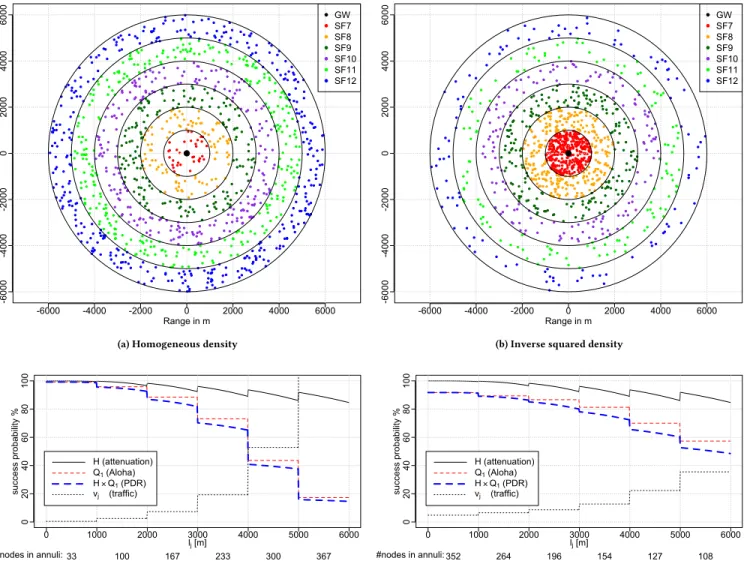
-6 00 0 -4 00 0 -2 00 0 0 2000 4000 6000 Range in m -6000 -4000 -2000 0 2000 4000 6000 GW SF7 SF8 SF9 SF10 SF11 SF12

(a) Homogeneous density

-6 00 0 -4 00 0 -2 00 0 0 2000 4000 6000 Range in m -6000 -4000 -2000 0 2000 4000 6000 GW SF7 SF8 SF9 SF10 SF11 SF12

(b) Inverse squared density

0 20 40 60 80 100 lj [m] su cce ss pro ba bi lit y % H (attenuation) Q1 (Aloha) H × Q1 (PDR) vj (traffic) 0 1000 2000 3000 4000 5000 6000 #nodes in annuli: 33 100 167 233 300 367

(c) PDR for homogeneous density. 300 nodes with PDR >80%

0 20 40 60 80 100 lj [m] su cce ss pro ba bi lit y % H (attenuation) Q1 (Aloha) H × Q1 (PDR) vj (traffic) 0 1000 2000 3000 4000 5000 6000 #nodes in annuli: 352 264 196 154 127 108

(d) PDR for inverse squared density. 809 nodes with PDR >80%

Figure 2: Comparison of spatial models,n = 1200.

SF allocation and showed that it performs the best with the equal-area-based SF allocation ranked second [19]. However, they did not take into account the capture effect important to evaluate the prob-ability of success reception under the LoRaWAN access method. The analyses assumed a constant node density within the range.

Note that the complexity of computing SF allocations increases with the order of allocations presented above: equidistant and equal-area-based allocations only depend on the distance, the SNR-based allocation requires solving Eq. 1 numerically, and PDR-based allo-cations lead to a nonlinear optimization problem.

The SNR-based allocation resulting from solving Eq. 1

numeri-cally for each j gives the values of ljpresented in Table 4 for three

values of threshold θ: 90%, 95%, and 99%. We can observe that increasing the threshold results in smaller cells.

The SNR-based and PDR-based allocations can be implemented in a similar way to the Adaptive Data Rate (ADR) algorithm de-fined in LoRaWAN. In ADR, the gateway estimates the average SNR level for the last 20 packets of a node. It then chooses SF and TP suitable for the given level of SNR, while keeping a 5 dB margin, and sends the parameters in the LinkADRReq frame to the node. In a similar way, the gateway can estimate PDR and choose the right parameters for the node. Nevertheless, such allocations re-quire sending downlink messages, whereas the gateways have very limited transmission capacity.

4.2 Inhomogeneous Node Density

We have already discussed the reasons for which assuming constant node density ρ for all annuli is not realistic. Moreover, the allocation of SF in LoRaWAN strongly impacts energy consumption so that far devices that need to use high values of SF will consume much

(6)

Table 4: SNR-based SF boundaries [km],H (lj) is the success

probability due to attenuation, fading, thermal noise.Sj/π

[km2]: value proportional to the number of devices. Node

density in an annulus based on the inverse-square law so

Sj/π × ρ(lj) is proportional to the number of devices.

SF7 SF8 SF9 SF10 SF11 SF12 l5 l4 l3 l2 l1 l0 lj : H (lj) ≥90% 2.23 2.68 3.23 3.89 4.54 5.30 Sj/π [km2] 4.96 2.23 3.24 4.69 5.49 7.47 ρj 1 0.69 0.48 0.33 0.24 0.18 Sj/π × ρ(lj) 4.96 1.54 1.54 1.54 1.32 1.32 lj : H (lj) ≥95% 1.84 2.21 2.66 3.20 3.74 4.37 Sj/π [km2] 3.38 1.50 2.19 3.17 3.74 5.1 ρj 1 0.69 0.48 0.33 0.24 0.18 Sj/π × ρ(lj) 3.38 1.03 1.05 1.05 0.9 0.9 lj : H (lj) ≥99% 1.18 1.43 1.72 2.07 2.41 2.82 Sj/π [km2] 1.40 0.63 0.91 1.33 1.55 2.11 ρj 1 0.69 0.48 0.33 0.24 0.18 Sj/π × ρ(lj) 1.40 0.44 0.44 0.44 0.37 0.37

more energy than devices with low SF, which will discourage the placement of nodes far from the gateway. There is also another adverse effect of using high values of SF: increased transmission times lead to more contention and collisions, thus affecting the probability of successful packet reception.

To take into account these considerations, we adopt a more realistic model for the spatial distribution of nodes based on the inverse-square law for node density:

ρj ρj−1 = l2 j−1 l2 j (7)

Table 4 also presents node density ρj for each annulus based on

this relation and the value proportional to the number of devices. To see the effect of the decreasing node density, we can observe that such a distribution favors the annuli close to the gateway with a higher number of devices using SF7 and results in less devices with SF 11 and SF12.

Figure 2 compares the spatial models—Figures 2a and 2b visualize the distribution of nodes for homogeneous and inverse squared density (n = 1200 nodes generated with a Monte Carlo method, randomly placed in equidistant annuli). We can observe that the number of nodes in the SF12 annulus is much lower for inverse squared density: 108 vs. 367 (see Figures 2c and 2d).

4.3 LoRaWAN capacity for different spatial

configurations

In this section, we present figures with PDR computed according to the model in Section 3. The total number of nodes (1200, 1700, and 2100) for the figures was chosen so that they give the maximal number of nodes that benefit from PDR > 80% for the respective SNR thresholds (we discuss this aspect at the end of this Section).

4.3.1 Equidistant SF frontiers.Figures 2a and 2c present the

spa-tial distribution of nodes and PDR in equidistant SF annuli for a

0 20 40 60 80 100 lj [m] su cce ss pro ba bi lit y % H (attenuation) Q1 (Aloha) H × Q1 (PDR) vj (traffic) 0 2228 3229 3889 4539 5299 #nodes in annuli: 487 151 151 151 130 130

Figure 3: Inverse squared density and SNR SF annuli for

H (lj) ≥90%, n = 1200. 787 nodes with PDR > 80%.

homogeneous density and n = 1200 nodes. The existing studies use this distribution and equidistance frontiers of SF allocation to analyze the LoRa capacity. Figure 2c shows PDR and its

com-ponents: channel attenuation H and Q1, the success probability

under ALOHA with capture. We can observe that Q1goes down

at each frontier because of increased traffic vjthat comes from an

increased number of nodes. As the annuli surface increases with the distance, the homogeneous node density results in the number of nodes in annuli growing with the distance and attaining 367 for SF12 with only 33 nodes using SF7. The estimated number of nodes that benefit from PDR > 80% is 300. The spatial model assumes that there are no nodes outside the last annuli.

Figures 2b and 2d present the distribution of nodes and PDR when the density of nodes is inversely proportional to the square of distance. PDR goes down with the distance much slowly than in Figure 2c because there are less nodes in higher SF annuli: 352 nodes using SF7 and 108 for SF12. The estimated number of nodes that benefit from PDR > 80% is 809. We can observe that the number of nodes in each annulus decreases with the distance.

This basic example shows the importance of the spatial model for evaluating LoRaWAN capacity: just changing the spatial distribu-tion of nodes raises the number of nodes with good PDR from 300 to 809. So, the choice of the spatial model may result in misleading results on LoRaWAN capacity and scalability.

4.3.2 SNR-based SF frontiers.Figure 3 presents PDR in SNR-based

SF allocation for the inverse squared density and n = 1200 nodes.

For H (lj) ≥90% threshold, the range of the cell is relatively large

with 5.3 km. 787 nodes benefit from PDR > 80% out of 1200.

Figure 4 and Figure 5 present the same data for H (lj) ≥95% and

H (lj) ≥ 99% thresholds and the total number of nodes n = 1700

and n = 2100, respectively. The increased value of the threshold

results in smaller cells (2.82 km for H (lj) ≥99%) because of the

dependance of funtion H on the distance. The number of nodes that benefit from PDR > 80% is 1115 and 1377, respectively.

We can observe that the assumption of the inhomogeneous den-sity results in an interesting effect: smaller cells can provide good PDR for an increased number of nodes. It evokes “cell breathing” in cellular networks in which heavily loaded cells decrease in size.

(7)

0 20 40 60 80 100 lj [m] su cce ss pro ba bi lit y % H (attenuation) Q1 (Aloha) H × Q1 (PDR) vj (traffic) 0 1836 2661 3204 3741 4367 #nodes in annuli: 690 214 214 214 184 184

H (lj) ≥95%, n = 1700. 1115 nodes with PDR > 80%. 0 20 40 60 80 100 lj [m] su cce ss pro ba bi lit y % H (attenuation) Q1 (Aloha) H × Q1 (PDR) vj (traffic) 0 1184 1426 1717 2067 2413 2817 #nodes in annuli: 853 265 265 265 227 227

H (lj) ≥99%, n = 2100. 1377 nodes with PDR > 80%. 0 20 40 60 80 100 lj [m] su cce ss pro ba bi lit y % H (attenuation) Q1 (Aloha) H × Q1 (PDR) vj (traffic) 0 1184 1426 1717 2067 2413 2817 #nodes in annuli: 371 167 242 351 410 559

Figure 6: Homogeneous density and SNR SF annuli for

H (lj) ≥99%, n = 2100. 776 nodes with PDR > 80%.

Note that the nodes benefiting from PDR > 80%, use low SF values: SF7, SF8, and SF9, which also means that their energy con-sumption stays low.

Figure 6 presents the results for a homogeneous density to com-pare with Figure 5: there are 776 nodes with PDR > 80%.

0 20 40 60 80 100 lj [m] su cce ss pro ba bi lit y % H (attenuation) Q1 (Aloha) H × Q1 (PDR) vj (traffic) 0 2646 3193 4082 4759 5232 #nodes in annuli: 555 174 215 147 96

Figure 7: Inverse squared density and PDR SF annuli for

H (lj) ≥90%, n = 1200. 460 nodes with PDR > 80%. 0 20 40 60 80 100 lj [m] su cce ss pro ba bi lit y % H (attenuation) Q1 (Aloha) H × Q1 (PDR) vj (traffic) 0 1465 2155 2598 #nodes in annuli: 1049 564 327 154

H (lj) ≥99%, n = 2100. No nodes with PDR > 80%.

4.3.3 PDR-based SF frontiers.For PDR-based SF allocations, we

use the Nelder-Mead simplex [20] to find arg max

l0..l5

min(H × Q₁). (8)

The optimization starts with the maximal range l0that we set

to the thresholds for two extreme SNR-based allocations: 5.30 km for 90% and 2.82 km for 99% (we skip the intermediate threshold of 95%), and looks for more uniform distribution of PDR values across SF annuli with the maxmin objective. We still assume the density of nodes inversely proportional to the square of distance.

Figure 7 presents PDR in the first case of a large cell: l0= 5.30 km

for 90% for the same total number of nodes as in Figure 3. Compared to Figure 3, the minimum value of PDR is higher (PDR > 60%), however, there are less nodes that benefit from good PDR > 80% (460 vs. 787).

Similarly, Figure 8 shows PDR for the small cell: 2.82 km for 99%. When comparing with Figure 5, we can see a similar effect— the minimal value of PDR is high (almost reaching 80%), but still the number of nodes that benefit from good PDR > 80% is low, which shows that the call has attained its capacity. If we lower the total number of nodes in the network to 1500, the maxmin PDR allocation gives very good results: Figure 9 shows that all nodes achieve PDR > 80%.

(8)

0 20 40 60 80 100 lj [m] su cce ss pro ba bi lit y % H (attenuation) Q1 (Aloha) H × Q1 (PDR) vj (traffic) 0 1426 2154 2574 2815 #nodes in annuli: 739 415 221 115

H (lj) ≥99%, n = 1500. All 1500 nodes with PDR > 80%.

0 500 1000 1500 2000 2500 3000 0 500 1000 1500 2000 Number of nodes N b. o f co ve re d no de s

Figure 10: Number of nodes with PDR >80% in function of

the total number of nodes in the network. Optimal

alloca-tion of annuli frontierslj as in Figure 9.

Note that the allocation exhibits strong asymmetry—it favors lower SF over high SF: there are 739 nodes in the SF7 annuli com-pared to only 8 nodes with SF12. As H is as high as 99%, the most

important factor for PDR is Q1, which depends on the traffic load

almost constant for all annuli with low SF (see Figure 9) in this allocation. Such an allocation has also an advantage of low over-all energy consumption as only a few nodes use SF11 and SF12, expensive in terms of energy.

4.3.4 Scalability. Figure 10 shows the number of nodes that benefit

from good PDR > 80% in function of the total number of nodes in the network for the small cell of the 2.82 km range. We fix the

allocation of annuli frontiers lj to the optimal allocation presented

in Figure 9 and we vary the total number of nodes. At the beginning, the number of nodes with PDR > 80% increases and achieves the maximum for n = 1500. Then, the number of nodes with PDR > 80% decreases because PDR begins to drop below 80%, which means that the network has attained its capacity.

A question remains: how does the SNR allocation perform com-pared to the PDR based one? Figure 11 shows the corresponding data for the SNR allocation. It achieves a lower maximum number of nodes with PDR > 80% (1377 nodes for n = 2100, see also Figure 5), but it can handle a slightly larger total number of nodes.

0 500 1000 1500 2000 2500 3000 0 500 1000 1500 2000 Number of nodes N b. o f co ve re d no de s

Figure 11: Number of nodes with PDR >80% in function of

the total number of nodes in the network. SNR allocation of

annuli frontierslj.

5 RELATED WORK

We briefly review previous work on modeling LoRa capacity and inhomogeneous spatial models.

5.1 LoRa capacity models

Georgiou and Raza [4] provided a stochastic geometry framework for modeling the performance of a single gateway LoRa network. They showed that the coverage probability drops exponentially as the number of contending devices grows. Their model assumes that the airtime is filled up—nodes use the shortest interval between packet transmissions allowed at given SF, which means that switch-ing to lower SF results in generatswitch-ing twice as much traffic. Moreover, the model of the access method corresponds to slotted ALOHA. In this paper, we have used the model with the modifications concern-ing the intensity of packet generation and the expression for the success probability reflecting the behavior of unslotted ALOHA.

Mahmood et al. [7] proposed an analytical model of a single-cell LoRa system that takes into account interference among transmis-sions over the same SF (co-SF) as well as different SFs (inter-SF). They derived the signal-to-interference ratio (SIR) distributions for several interference conditions. Due to imperfect orthogonal-ity, inter-SF interference exposes the network for additional 15% coverage loss for a small number of concurrently transmitting end-devices.

Li et al. [5] analyzed interference in the time-frequency domain using a stochastic geometry model assuming transmissions as pat-terns on a two-dimensional plane to quantify the capture effect. They use the model to analyze LoRaWAN by characterizing the outage probability and throughput.

Based on a simple model for collisions and capture effect, Cail-louet et al. [9] introduced a theoretical framework for maximizing the LoRaWAN capacity in terms of the number of end nodes.

All the presented models assumed a homogeneous node density around a gateway.

5.2 Inhomogeneous spatial models

Gotzner and Rathgeber [10] challenged the homogeneous assump-tion in spectrum frequency analysis and proposed to model the

(9)

spatial inhomogeneity of real cellular traffic with log-normal distri-butions.

Lee et al. [11] observed that modeling and simulation of a cellu-lar network typically assume the target area divided into regucellu-lar hexagonal cells and a uniform distribution of mobile devices scat-tered in each cell. In reality, the spatial traffic distribution is highly non-uniform across different cells, which requires adequate spatial traffic models. They reported on traffic measurements collected from commercial cellular networks and demonstrated that the spa-tial distribution of the traffic density (the traffic load per unit area) can be approximated by the log-normal or Weibull distribution depending on time and space.

Mirahsan et al. [12] used maps of Paris, France to study the spatial traffic heterogeneity of outdoor users in dense areas of the city center. They found that the statistical distribution of spatial metrics is close to Weibull. Their results show that the building topology in a city imposes a significant degree of heterogeneity on the spatial distribution of the wireless traffic.

Taufique et al. [14] investigated the problem of planning future cellular networks. They noticed that the cell size increasingly adapts to the spatial traffic variation. Instead of having the same cell size throughout, areas with low traffic density can have larger cells compared to areas with high traffic density, resulting in energy and cost savings. As planning future cellular networks faces heteroge-neous and ultra dense networks, the issue is to find the optimal base station placement jointly for macrocells and small cells in a non uniform user density scenario. They showed an example of such a deployment for a Gaussian spatial user distribution.

Wang et al. [13] characterized temporal and spatial dynamics in cellular traffic through a big cellular usage dataset covering 1.5 million users and 5,929 cell towers in a major city of China. Their results reveal highly non-uniform spatial distribution of the traffic density.

6 CONCLUSIONS

In this paper, we have shown that adopting inhomogeneous spatial node distribution leads to much different results on LoRaWAN capacity than that reported previously. The existing measurement studies of the traffic density in cellular networks showed high diversity of the node density in urban settings. We expect that LoRaWAN networks will follow the same deployment pattern with the placement of gateways close to high density areas.

We have used the model by Georgiou and Raza [4] to analyze the capacity of a LoRaWAN cell for various types of SF allocations: equidistant, SNR-based, and PDR-based. We can draw several con-clusions from the numerical results presented in this paper:

•For a required PDR level and a target communication range,

we can find an allocation of annuli lj that results in the

maximal number of nodes that benefit from the PDR level.

•There is a natural trend towards configurations composed

of smaller cells that concentrate nodes close to the gateway.

In this way, nodes benefit from low SF, which also means lower energy consumption.

• To provide the required PDR level to more nodes, we need

to consider multiple gateways that will increase the overall capacity while maintaining moderate energy consumption. In future work, we plan to explore a model in which the density of nodes is a continuous distribution in function of the distance from the gateway, which may better reflect realistic deployment scenarios.

We also want to develop models for capacity prediction in case of multiple gateways.

ACKNOWLEDGMENTS

This work has been partially supported by the French Ministry of Research project PERSYVAL-Lab under contract ANR-11-LABX-0025-01.

REFERENCES

[1] LoRaTM_{Alliance. A Technical Overview of LoRa and LoRaWAN.}

[2] A. J. Berni and W. Gregg. On the Utility of Chirp Modulation for Digital Signaling. IEEE Trans. Commun., 21, 1971.

[3] Nicolas Sornin. LoRaWAN 1.1 Specification. Technical report, LoRa Alliance, October 2017.

[4] Orestis Georgiou and Usman Raza. Low Power Wide Area Network Analysis: Can LoRa Scale? IEEE Wireless Commun. Letters, 6(2):162–165, 2017. [5] Zhuocheng Li et al. 2D Time-Frequency Interference Modelling Using Stochastic

Geometry for Performance Evaluation in Low-Power Wide-Area Networks. In 2017 ICC, May 2017.

[6] Antoine Waret et al. LoRa Throughput Analysis with Imperfect Spreading Factor Orthogonality. IEEE Wireless Communications Letters, 2018.

[7] Aamir Mahmood et al. Scalability analysis of a lora network under imperfect orthogonality. IEEE Trans. Industrial Informatics, 15(3):1425–1436, 2019. [8] Martin Heusse et al. How Many Sensor Nodes Fit in a LoRAWAN Cell? submitted

for publication, 2019.

[9] Christelle Caillouet et al. Optimal SF Allocation in LoRaWAN Considering Phys-ical Capture and Imperfect Orthogonality. In 2019 IEEE GLOBECOM Conference, 2019.

[10] U. Gotzner and R. Rathgeber. Spatial Traffic Distribution in Cellular Networks. In VTC ’98. 48th IEEE Vehicular Technology Conference. Pathway to Global Wireless Revolution (Cat. No.98CH36151), volume 3, pages 1994–1998 vol.3, May 1998. [11] Dongheon Lee et al. Spatial Modeling of the Traffic Density in Cellular Networks.

IEEE Wireless Commun., 21(1):80–88, 2014.

[12] Meisam Mirahsan et al. Measuring the Spatial Heterogeneity of Outdoor Users in Wireless Cellular Networks Based on Open Urban Maps. In 2015 ICC, pages 2834–2838, 2015.

[13] Xu Wang et al. Spatio-Temporal Analysis and Prediction of Cellular Traffic in Metropolis. In 25th IEEE ICNP, pages 1–10, 2017.

[14] Azar Taufique et al. Planning Wireless Cellular Networks of Future: Outlook, Challenges and Opportunities. IEEE Access, 5:4821–4845, 2017.

[15] Semtech. SX1272/73 - 860 MHz to 1020 MHz Low Power Long Range Transceiver, 2017. URL https://www.semtech.com/uploads/documents/sx1272.pdf. [16] Jetmir Haxhibeqiri et al. LoRa Scalability: A Simulation Model Based on

Interfer-ence Measurements. Sensors, 17(6):1193, 2017.

[17] Claire Goursaud and Jean-Marie Gorce. Dedicated networks for IoT : PHY / MAC state of the art and challenges. EAI endorsed transactions on Internet of Things, 2015.

[18] Takwa Attia et al. Experimental Characterization of LoRaWAN Link Quality. In 2019 IEEE GLOBECOM Conference. IEEE, 2019.

[19] J. Lim and Y. Han. Spreading Factor Allocation for Massive Connectivity in LoRa Systems. IEEE Communications Letters, 22(4):800–803, April 2018.

[20] J. A. Nelder and R. Mead. A Simplex Method for Function Minimization. The Computer Journal, 7(4):308–313, 01 1965.