Effects of the Dynamic Characteristics of a Vibration on the Forced Vertical Vibrations of Piles

Publisher’s version / Version de l'éditeur:

Technical Translation (National Research Council of Canada), 1971

READ THESE TERMS AND CONDITIONS CAREFULLY BEFORE USING THIS WEBSITE.

https://nrc-publications.canada.ca/eng/copyright

Vous avez des questions? Nous pouvons vous aider. Pour communiquer directement avec un auteur, consultez la

première page de la revue dans laquelle son article a été publié afin de trouver ses coordonnées. Si vous n’arrivez pas à les repérer, communiquez avec nous à PublicationsArchive-ArchivesPublications@nrc-cnrc.gc.ca.

Questions? Contact the NRC Publications Archive team at

PublicationsArchive-ArchivesPublications@nrc-cnrc.gc.ca. If you wish to email the authors directly, please see the first page of the publication for their contact information.

For the publisher’s version, please access the DOI link below./ Pour consulter la version de l’éditeur, utilisez le lien DOI ci-dessous.

https://doi.org/10.4224/20386756

Access and use of this website and the material on it are subject to the Terms and Conditions set forth at

Effects of the Dynamic Characteristics of a Vibration on the Forced

Vertical Vibrations of Piles

Shekhter, O. Ya

https://publications-cnrc.canada.ca/fra/droits

L’accès à ce site Web et l’utilisation de son contenu sont assujettis aux conditions présentées dans le site LISEZ CES CONDITIONS ATTENTIVEMENT AVANT D’UTILISER CE SITE WEB.

NRC Publications Record / Notice d'Archives des publications de CNRC:

https://nrc-publications.canada.ca/eng/view/object/?id=555fad22-ad0c-44f0-833e-024ea707a5a5 https://publications-cnrc.canada.ca/fra/voir/objet/?id=555fad22-ad0c-44f0-833e-024ea707a5a5

NATIONAL RESEARCH COUNCIL OF CANADA

TECHNICAL TRANSLATION 1502

THE EFFECTS OF THE DYNAMIC CHARACTEID5lf1€S

OF A VIBRATOR ON

THE FORCED VERTICAL VIBRATIONS

OF

PILES

BY

O. VA. SHEKHTER

FROM

TRUDY NAUCHNO - ISSLEDOVATEL' SKOGO INSTITUTA OSNOVANII I FUNDAMENTOV DINAMIKA GRUNTOV

SBORNIK. (27) : 58 - 79. 1955

TRANSLATED BY

V. POPPE

THIS IS THE TWO HUNDRED AND SECOND OF THE SERIES OF TRANSLATIONS PREPARED FOR THE DIVISION OF BUILDING RESEARCH

OTTAWA 1971

which contain soils with inadequate strength or undesirable

deformational properties. Such foundations often represent

a considerable proportion of the total construction costs; improvements in installation methods might therefore result in considerable savings.

The Division of Building Research has maintained an interest in the performance as well as in the method of installation

of pile foundations. Exploratory measurements carried out by

members of the Division on the vibratory effects of pile driving have established the need for a more realistic theoretical

treatment of this complex phenomenon. This translation is

made available in the hope that the present work may provide

a basis for a better understanding of the pile driving phenomenon and permit a more rational quantitative treatment of the

subject.

The Division is grateful to Mr. V. Section, National Research Council, for and to R. Ferahian of this Division who

Ottawa

December 1971

Poppe of the Translations translating this paper checked the translation.

N.B. Hutcheon Director

Title:

TECHNICAL TRANSLATION 1502

The effects of the dynamic characteristics of a vibrator on the forced vertical vibra-tions of piles

(Zavisimost' amplitudy vynuzhdennykh vertikal'nykh kolebanii svai i shpunta ot parametrov vibratora)

Author: O. Ya. Shekhter

Reference: Trudy Nauchno-issledovatel'skogo Instituta

Osnovanii i Fundamentov. Dinamika Gruntov. Sbornik, (27): 58-79, 1955

Translator: V. Poppe, Translations Section, National Science Library

1. Introduction

The paper examines the relation between the vibratory character-istics of piles driven into soil by vibration and the ｣ｨ｡ｲ｡｣ｴ･ｲｩｾｴｩ｣Ｓ

of the vibrator, i.e., the driving moment and number of revolutions. The first experimental study of this relation was carried

out by D. D. Barkan, V. P. Sukharev and V. N. TUPikov(l) in 1951. They found that the linear vibration theory, according to which the bearing capacity of soil is assumed to be proportional to the displacement, is not always in agreement with experimental data on the relation between the amplitude and frequency.

The resonance curves obtained in these experiments referred

to a small range of rpm. The curves which extrapolate experimental

data beyond this range are somewhat arbitrary, especially if we consider that the frequency range in the experiments was an un-stable zone.

Owing to the fact that individual experiments in this field invariably produce some erroneous data, generalizations can be made only on the basis of a large number of experiments.

Our tests involved the sinking of 170 piles (12, 15, 20, 25 and

31

cm in diameter) and 2 sheet piles (ShP and ShK) about

4

m

in length. The cross-sectional areas of sheet piles were 70 and

60 cm2 _{respectively. (For description of experimental site see}

the article by N. A. Preobrazhenskaya in this collection of papers).

The total weight of the vibrator was 700 kg, and the maximum eccentric moment 660 kgcm.

The amplitude of vibrations and the power used by the motor of the vibrator were determined for four values of the driving moments and revolutions up to 1700 rpm.

The amplitude and power changed relatively little with depth, which was evidently due to specific geology and relatively small

depth of sinking. Geology and testing techniques are described in the paper by Preobraznenskaya.

2. Theoretical Resonance Curves for Different Hypotheses of the Bearing Capacity of Soil

To find the relation between the amplitude of soil vibration and the characteristics of the vibrator, i . e . , the driving moment and rpm, let us examine the simplest case, i.e., the vibration of mass with one degree of freedom. Let us represent the bearing capacity of soil in the form of two components:

where R 1 (z ) is the component dependent on the displacement of z .

,

ｒＲＨｾＩ is the component dependent on the vibration rate, i . e. , the damping force or force of friction.

Let us examine the following cases:

1. R1(z) is nonlinearly dependent on z, while ｒＲＨｾＩ is proportional to velocity (viscous friction).

2. Various hypotheses concerning damping forces ｒＲＨｾＩ during displacement proportional to R(z).

3.

Forced vibrations of a pile during separation from tne soil.

First case. In a conventional linear theory, R1(z) is assumed to be proportional the the displacement, which is true for small amplitudes.

However, in the case of a vibrator with a large driving moment, the amplitudes may be fairly large, and therefore the relation

of R1(z) to the displacement must obey a more complex law, e.g.:

•

=

az the equation for the vibration is as follows:

.J .. -/

R( )

+'

ｑｯｾＢ

t

- Z -

z

az

= - -

llr

sin

00 1

g ,f!

where

ｑｾｅ

w2 _{is the perturbation force of the vibrator; Q is the}

g

weight of pile and vibrator, including the motor, etc.

On

､ｩｶｩ､ｩｮｾ

the equation by

ｾ

_po we obtain:

z

+

1-.2_{Z - 1Z;\}

+

_OZ5

+

_2nz

₌

_A

_.,002

_sin

_wt;

₍

₁₎

A

= Qot (2)

., Q'

Let us take the following equation as a first approximation:

'If

, '-b

Z

=a

sin oot - b cos

wt

=

A sin (rot

+

e],

tg

9 L - - ,(3)

"

then

ii = -

).2Z

+

TZ:; -

3z

6 -

2nz

-t-

A

.ro2

sin

mt.

.(

4)

On substituting equation

(3)

into the right half of

(4)

and replacing the squares, cubes and products of trigonometric factors by their expressions in terms of higher harmonics including the

fifth, we obtain after ｩｮｴｾｾｲ｡ｴｩｯｮＧ

Z • _.#

(-)2

3 .. 3

00

₂ 5... , 10

CQ Z= Sinｾ "" - - -

"fa' -

-

.,

+ -

ｯ｡ｾ --+- -

a

3

b

2 ..L

4 ' . ' 8 1 8 '

+ :

ab

f

+

24.-

A.U)Z)

+

coswt(-

b"A"!

+

+

-ra'lb

+

+..!

111' -

Ｍｾ

lafb -

ｾ

a

1

_{/r -}

Ｍｾ

_If>

-t-

_2tteDa)'

ＭｾＭ

.. 8 8 8 '

+ .

_Stn

3 t

(la' 3141"1 6

ｾ

/)

+

1Oa'bl

ｾ

+

16

' b

4)

+

(l) - - - - Q Q (}

-·-oa

36

36

144

144

144

( 5)

ｾ

COS

3mt

(--3

l

a

2b

+

ｾ

+

..!!.

Qa4

_b

+

_.2Q..

aa

2

b

_{3 _}

ｾ

8b

_{6 )}

+

I 36 36 144 - 144 144 sin5w! " . 'I ? , - I _ en c:Su-'! • I - ; " ,.

+

0

(ad -

1

Ga"

b

w -1-Dab) i --- ---- r.ｾ -

5a

ｾ

h

Ｍｾ j

Oa

2

b

3 - biJ ) .

400

4 0 0 '

Let us define a and b such that the coefficients of sin wt and cos wt will be identical for

(3)

and

(6)

giving:

a

=.2-.

(aA7! -

ｾ

"'aA2 4 -

ｾ

oaA4

ｾ

2n.iJlb -

A

0)2).

(1)2 4 ' I 8 I . . . ,

- b=

ｾ

(-

b).2+ : lbA2 -

:

｡｢ａｾ

+2nma)

(6)

or

a

(A.:! -

Q)S)

_..!

laA2·t

ｾ

SA"

-L

2nmb - A 0)2-=0·

4 8 I - ,

- b

ＨＱＮＮｾ

-

m!)

+

..!-lbA2 -

ｾ ｩＩｨａﾷＭｌＲｾｾ

=

O.

..

ｾ (7 )

From this we find a and b, which we shall identify with subs cript I:

Then the coefficients at high harmonics for sin and cos will be as follows: IZ

I

' 2 . '

ｾ｜

' 5 It t·· . . , 0 2

b

2

+

3b

4) ] •

a,..

ｾ

1l

a. _..

3D,.

r

-4-Q , -

a!

1"

"aJ

I I t

｢Ｎ］ＭｾＮＫＨ

｢ｾ

-3an

+ :

a(-

b:

+

20;

｢ｾ ＫＳ｡ｾＩ

];

4!f - : : . ,

(a: -

tooibi

+

SbH

ｾ

(9 )

b

₅

=

ｾ

(-b1+IOarbi-54t);

,

ｖ｡ＲＫｾＮ

A

- I f

ｮｾ

+'

M

= -..'

ａｾｩｬ

-

ＮＡＮｾａｩＩ［

. , I

=

1 1, I -

V

ｾ ! 3 6 . : ' \ 4 , . - t _a

A.=Vai

+

'1

=

400-!

Aa'

and consequently the displacement will be

r

=

(a

_l

sin

mt -

'''1

cos .t)

ｾ (G,

sin

ｾｦ ._.

/1,

cos

ｾｬｬＬＩ

+

(a.

sin

Smt -_.

｢ｾ

<:C5

5et) .

ai

+

p'i=

Ai;

(10) ( 11 '- ) From

(8)

we obtain:

A2

=

_

4n2- '

+ (.., -

).2

+ :

lA' -

:

ｾａＴ

r '

(12 )

(in the case of Al subscript 1 will be omitted).

For the phase shift of the first harmonic we have:

(13)

:In-3 5 - , (1)2- 1..2

+

- r

A2 -

-aAf

4 8

tg

ｾ

=

_-_bl_

=

---:.----=-at hence . b1 2nA StOlP=

--=--;---• A A .... ·

Let us assume for the sake of simplicity that

3 ,5 ｾｾ .. \' = -

1 - ---.

0,,'" ". ｾ .. ｾ l

4

ｾ

- ,.,.

ｾ X , - " ,.. ( 1

4 )

Then, on solving (12) with respect to w2 , we obtain

J-=

..1''',.% -

Al -

_.!..)

-+- A

1/

A2

ＨｊｌｾａＲ

ＮＩｾ

_

ａﾷ｟ｾ

f);-

A2 .r ') \ ?

2....

Y

-.'

y . x - \" .- y -

7.

A2 _ A2

00

Let us proceed to generalized coordinates. Let

., -in' A 3 jA:" ｾ］ｾ［ Q = - -

.

₁₁₌

A.

,

----I,

"

ｾＡ

S

&A-4

-ｾ］ｵ

- a

2v, III

'0=-.

_At

,

.

(t)=

-

_{(16 )} 8 ).

then

;2

= ....

ｾ

I{a'

(I -

4' -

t)

±

II

V

(1-

a,)2- Ea

2(

1 -

｡ｬｾ

-

-t)}.

on

at ｾ

=

0 - ＮＨＱＭｾ

..

-

- - . ; " ' - - -

...

41

+

I (17' )

One o£ the limits of ｾＲ at a + 1 will evidently tend towards

jnfinity Ｈｾ

=

00).

The second limit of ｾＲ at a + 1 will be

11m

";1_

(1 - ｾＩｉ

.-1

2(1-P-

ｾＩ

.

In abstract coordinates equation (10) will assume the following form: A. { - ,

A . _

4 . . . -- ; ,

at a?

+ .' -

I j;

b

₁

=

--;J

a%.,.. ;

a: =-

.!!.. [

ｾ

(

ｾ

-3b!)

.-.

t' - ( _

trl

+

2a

2

ｾ

+

ｾＩ

].

.... .: 21A2 -1 1 · JＸａｾ I I 1 l ' ｾ

.

b

3

=

ｾ

r---

(b: -

3a

2)

-t-

V

(-b!

+

2a

2

b?

+

34

4) ] :

..z

21...

ｾ 1 1 · ＱＸａｾ J J 1 1 · 'I. Q.

=

_GJt'_

ＨｾＭＱＰ｡ＲｾＫｾﾷＩ

.

.. - 4 1 11 1 · ｾａ

.

-ＨｾＭｬｏ｡Ｚ｢ｩ

+

San;

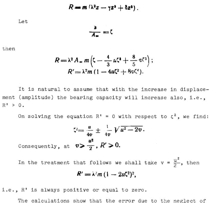
(17")

To avoid possible incompatibility, let us examine the relation between the bearing capacity of soil and displacement.

Let

then

R=)..2A ...

ｭＨｾＭＫｵｾＧＫ

:

'V

l 5) ;

R'=

)..2

m

(1 - ＴｕｾＲ

+

ＸＧｴＧｃＮｾＩＮ

It is natural to assume that with the increase in displace-ment (amplitude) the bearing capacity will increase also, i.e.,

RI > O.

On solving the equation

HI

=

0 with respect to

S2,

we find:

"2 _ _

.. _

!!-

+

I

-

V

u - v .

2

2

40 - -tv

ｵｾ

Consequently, at

V:>

T'

R'

:>

O.

In the treatment that follows we shall take v

i.e., RI is always positive or equal to zero.

u2

=

2 '

then

The calculations show that the error due to the neglect of

the third harmonic does not exceed 20% of the value of the amplitude

for u

=

8,

and is considerably less for other parameters. The

error due to neglect of the fifth harmonic is quite negligible. Therefore, additional harmonics may be ignored.

Figure 1 shows thE resonance curves calculated from (17).

u2

In every case v

=

2'

If we use the first harmonic only, then the instantaneous power will be equal to:

w

and consequently, the power for the cycle of vibrations T

=

will be equal to:

2n w

r

w==J..fw

pt=

T

t

J.na't

AIJftQ K

(18)

Figure 2 illustrates the relation between power and frequency at different values of the attenuation coefficient for two values of u:

u

=

O(v

=

0) and u

=

0.5(v

=

0.125).

Second case. Let us now examine various hypotheses concerning

the friction forces.

The general form of the vibration equation for any relation between damping forces and velocity ｦＨｾＩ is as follows:

.z

+

f(z )

+

In

=

Q,a.

,.2

sin

-I.

K Let us denote:

•

1.'- _ .

- . t

,(z)=

/(z)

•

and rewrite equation (1):

.- +,

｜ｾＩ

+)". -

A.co· sin

c»t .

There is no precise solution of this equation. For an

approximate solution use is made of the equivalent equation with linear attenuation(3): (20) where a:

2n=-- ;

m '2 It A = - . m

The solution

bf

this equation is as follows:

z

=

A

sin

(wi -

ｾＩ［

A

·,

w-oo

We also assume that the work of damping forces within a vibration cycle ｾｮ equations (19) and (20) is the same, i.e.,

r

T T

IV

=

l/(it

dz=

1/

{z )zdt-

i

ClZ

2

dt .

On caleulating the integrals for a vibration cycle, we

evident ly have

and

If we take fez)

= SzP

(the sign of

S

must be such that the friction force would counteract the movement), then on sUbstituting into T I

I

fa

%%

dt

=

ｾ ｾ

Z"+

1

dt ,

we obtain \,'t· (22) where

The values of coefficient yare given below. 1

o

4

-

_&

1.1

1284

1

I I

I

2

I

J

..

I

5 6

I

• 8 3 32 5 64

a;-

₄

_T5i"

_T

Ｓｾ

On substituting the values of a from (22) into (21), we m

obtain:

where

(24)

(25 )

After simple algebraic transformations we obtain from equation (10): At P we have 1 =

2":l

on denot ing

..

2/!]'

CIt '--lIA. J •

==

T'

(26)

From equation (26) at w : A, we obtain

A A

-

wi I

-

=

--=---=--=

2C .

Figure 3 shows the resonance curves for two values of p:

p

=

ｾ

and p

=

2

Let us examine a combination of dry and viscous friction.

A precise solution was given by Den Hartog(4). However, we

cannot use his resonance curves because in our case the perturbation force is proportional to w2

• Since the differential equation is

nonlinear, there will be no simple proportionality between the

perturbation force and the amplitude. Therefore, all curves have

been recalculated. Den Hartog's conclusions are briefly as

follows. In the presence of dry friction, we should distinguish

between motion without stops (Figure 4a) and motion with one or

several stops (Figure 4b). The stops result from the fact that

the perturbation force cannot overcome the friction force and the bearing capacity of soil.

In the case of simple motion without stops, the differential vibration equation may be expressed in conventional terms through-out the entire period of time:

mz

+

kz

+

F

+

a z

= Vo' &1.)2

Cps (

wt

+

ep) •

g

In the half-period ｏ＼ｴ＼ｾ the velocity is negative, and w

therefore for this interval F must have a minus sign.

The phase shift between the perturbation force and the friction force is defined by angle

¢

calculated from boundary

conditions which will be discussed later. Let us divide the

equation by m

=

Q and introduce the following terms: g F _

.f...- '\

2 __

svz,

- - I\. -J'" m

k

A -

QOE • • - Q ' a

-=2n.

m

Then within the interval O<t<TI equation (27) will have the

w

following form:

Z

-1-)..2

(z

-f)

+

2n

z

=

A...

(1)2COS

(rut

+

ep).

(29)

Let

p

=

y'-::i _

n2;

q

=

_I

l/(k:t _

0)2)01

+

ＴｮＱＰＩｾ

;

u

ql.2

COS1 =().:! - CI)!)'COSｾ

+

2nO) sin

<p;

qAt

sin.

= ().2 - w2)

sin

ep -

2nQ) cos

ep •

(30)

The general solution of this differential equation is as follows:

A . !

Z -

ｾＭＢＧＨｃｉ

cospt

+

C

_J

sinpt)

+

ｾａＲＭ

COS

(ott

+

e)

-+

f ,

(31)

The three arbitrary constants Cl, C2 and ｾ are found from

four boundary conditions including one other unknown A which, consequently, is also found from these equations at t

=

0, z

=

A, z

=

0 and

ｴ］ＭｾＮ

z=-A,

Z-O.

•

Without going into detail, let us represent the solution of this equation in a form which differs somewhat from that used by Den Hartog'

ｾ｟Ｎ

r

ＱＮＮＨｾＩＮ｟

(

I

)%

fP -

.i:

a,

(32)

A.

V

t'

1

A.

A.

n

sin4-•

1UC ,..

ch--+cos--•

•

it

H = - · - - - ·

,.

.

where sb

ｾ

-

..!.

sin

p::.

G=

•

II • cb

ｾＫ｣ｯｳ

I"

•

•

.

,

sina=

sin

¢

and cos

¢

are

Ｍｴｬｾ

fH;

COSI= .}2

(A

+

Of):

ａ｟ｾ ａ｟ｾ JI

found from (30).

Let us now examine the case of motion with one stop. We shall assume that the stop starts at t = to.

The differential equation for the section from 0 to to has

the same form (29) as for the case of continuous motion.

There-fore, its general solution is also given by equation (31). The boundary conditions are similar:

at t = 0, z = A, z

=

0,

.

at t

=

to, z

=

-A, z

=

O.

In contrast to the preceding case, the equation will contain the unknown factor to. The additional ratio for its determination may be obtained i f we observe what happens at the beginning of motion t

=

O.

Since at this moment the mass is at rest, velocity and acceleration are equal to zero, i.e., ｾ = 0 and

z

=

o.

In this case the differential equation (27) has the following form:

kA - F -

Qoe (1)2COSCD

=0

• g or A (1)1

A

-/=

eo

cos e.

(

35)

AI

All unknowns are found from equations (34) and (35): C1 ; C2 ; ,4>; A and to.

We shall omit the intermediate calculations and proceed directly to the solutjon of the differential equations for the section ｏｾｴｾｴｯＺ

A

f

(})!

T

_{.._} ］ＭＫＭｃｏｓｾ［ _{A. I,t}

sin,

-= Aqt .

COS

cp _

__8..=-"..".,.",...==

}r(Aqt)!

+

(Bql)" - } , r

{Aqt)t

+

(Bqt)!

Aqll

=-

(1 -

-ii-

r,,4sln

.t, -

Ｒｾ

..

e-'ecos

(Oto-t-

2:

1 01

cospt

_o

+

(

36)

+

fit

(211

1 . . ,

1)'

t

P

) . t

-to

AI -

sin

Po;

B

q

2= -

2ft-

e-t.

sin

tal, -

(1 -

.s)

e-

/o

cos

-to

+

II ;"2 i

+

(I

ＭｾＩ

cospt, +...!..

(I

ＫｾＩ

slopt,.

AI

p

12

COS £ and sin £ are found from (30) and to from the transcendental equation:

2l"1)! ( COSI \ I

A:-.I

=

-COS,

+

e-at·cospt.

q

-

COS

9

) ' \

+

rat.

sin

pt

0

(...!!..

cos

s -

ｾ

COS? -

ｾ

Sin!) - _1 COS

(-to

+

e}.

(3

t:

IIIl P pq q

This equation cannot be solved directly with respect to to at given f and w. It can be solved by the graphoanalytical method.

If to and ware given, we can find A and f analytically from

(35)

and (37). Then for a given w we can construct two sets of curves

(A, to) and (f, to) from which we can find to for the given A

and f. At to

=

ｾ we obtain the boundary between the two solutions. w

Figure

5

shows the resonance curves for one case of viscous friction

I

=

0.5 and different values of dry friction f calculated

from precise equations. The dotted line in Figure 13*represents

the boundary separating the region of motion with one step from the region of continuous motion.

The curves in Figure

6

illustrate the case where viscous friction is absent, 1.e., ｾ

=

o.

The continuous resonance curves have been constructed from c.pproximate equations. The dotted lines and individual points indicate the points of ｲ･ｳｯｮ｡ｾ｣･ curves calculated from precise equations.

The form of the approximate solution is simple, and closely resemb les that of the precise equation:

1-(

ｾ

r

( 38)

Third case. Forced vibrations of a pile with separation

from the soil.

We shall examine the simplest case where the action of soil on the pile is replaced by the reaction of a spring (inertialess) with rigidity c, while the mass is assumed to be concentrated at a point.

Let Xl denote the position of this point during its motion

on separation from the soil (spring), and X2 denote the position

when the point is on the soil (spring). Let the boundary between

these positions (Xl

=

X2) be the start of the coordinates.

Let us assume that steady-state motion with a period which

is a multiple of the period of induced force enT

=

2nn, where w

w

is the frequency of the induced force) is possible.

As is usually done in the case of vibrators, let us represent the induced force as follows:

p=

ｑＮｾ

U)!

sin

(lOt

+

9)

1

g

where Qo is the driving moment of the vibrator and

¢

is the as

yet unknown phase shift between the induced force and the separation moment.

Let us assume that in the time interval ｏｾｴｾｴｬ the pile moves while separated from the soil (t

=

0 is the separation moment, t

=

tl is the moment of impact with the spring). If Q is the weight of pile, then the differential equation of its motion in this time integral will be as follows:

..

Q

_x··

QtJl."..

( t '

)

K I

=

g.-

sin

(I)

-r'

+

Q;

( 39 )

Let us assume further that at

ｴｬｾｴｾＲｔｉｮ

the pile vibrates to-w

gether with the spring*. The differential equation of its motion

in this time interval will have the following form:

The differential equations

(39)

and (40) must be integrated at the following boundary conditions:

at

t-=O,

x1=o,

1

at

t

===

t

J1 Xl

=Xt

=

0,

ｘｾＨｴｬＩ

-

x;

(ti),

t -

2r.n

•

at

-

,

X,=O

r

₍₄₁₎ (I)

J

and at

X;

₍₀₎

=

ｸｾ

(2

1t: ).

It is assumed under such conditions that the fall of the pile to the ground occurs without sudden changes in the rate of fall.

Hence, altogether there are six boundary conditions. Let

A

_{. -}

_

(Joe_Q

k=

--=-

)..2A

C=-.

A

g ' w (42)

*

We could have assumed in a more general case that the pile

would separate from the soil more than once within this period. However, it was found experimentally that the separation occurs within the first, second and third periods of the induced force.

Then a general solution of equations

(39)

and

(40)

will have the following form:

x. . (

t

+ )+

t;t2 I at I b

A

= -

Sin w t;> ,; - T - .- i - - )

0

-<

t

-<

t

1

ee ＮｾａＮ A"" A.

i:-- -

1 ..

sin(-t

+

t;»

Ｍｾ

_1

+

ｾ

sin

At

+

.s:

cas

At,

(43)

.... I - I . ! k A. A..,

t

₁

<l

t

4

2&n •

•

where

The six unknowns

(a,

b, c, d, ¢, and tl) are found from the boundary c ondi tions given ab ove .

The unknown time tl is determined from the following trans-cendental equation: (44 )' a : cos '"

+

sin, cg -2 ( y- a ｾＩ -'.-" _L.

tg -- .

(1 _ :') ｾＩ I "l

k =

-where

U

l

=

14':

=

:tDt

1;

flit.

=

21tn't

.

For ¢ we have the following expression:

:t ..I,

- . = - - -

_{. 2 :!} or ｾ］ＭＭＭ Ｓｾ 11I/.

·

2

2

Here the value of

¢

is such that k is positive. Finally:

A:

=M(COS

ｾＫ

tg ; Sin

Ti) ;

M =

-k(tgftgcp+C)

e

'

a )

- ］ｾ

A-flsin

Yi -

tg-

cos

Ti ;

A., \

2

Tj't

.--tg,- ..

2 b .

--:;r-

=

SID ｾ［

-•

-A._

The pile velocity at the moment of separation from the soil ( t

=

0 or t

= ---

2TIn ) .lS glven• by: W f1

"ltt

--:-- = -

COSq:> -

-A.u>

2k .

The pile velocity at the moment of impact with the soil (t

=

t l ) is equal to but has the opposite sign than the velocity

at the moment of separation.

The physical meaning of the problem evidently demands that

If this condition is not satisfied, then the solutions are nonsensical, although they satisfy all boundary conditions and differential equations.

It is readily seen that Xl and X2 in the solution obtained

will be symmetrical with respect to the middle of their sections. The investigation of the solution obtained is made difficult by the transcendence of the equation.

The resonance curves should be constructed by taking k for

a number of values of s to find T, which does not have to be single-valued, and then by using equation

(5)

construct the curve of

corresponding motion, from which the vibration amplitude could be determined.

If k is given, T may be found from the k curve.

two values of n. The dotted sections correspond to

Consequently, the solutions for these sections have

Figure

7

shows the k(s) curves for various values of T and

f

...Y-}

t = t 1<0 •

AooW

no physical meaning.

As may be seen from the curves, k for certain nand s is a very complex function of T.

Figure

8

shows the curves of pile motion under different

conditions. It may be seen that there are large variations in

Shown data.

3.

shown

Comparison of Experimental and Theoretical Resonance Curves

The circles on curves in Figure 9 indicate the experimental The frequencies w

=

0.014 N (N - rpm of the vibrator) are

A

along the ab s ci s s a , while the relative amplitudes are A

oo

along the ordinate.

On comparing experimental and theoretical data we may con-clude that the experimental data are best approximated by theoret-ical curves with allowances for the highest terms of expansion

in the bearing capacity of soil and introducing one more coefficient a .₀₀

The experimental values of amplitudes for high driving fre-quencies of the vibrator tend towards values less than the

theoretical

Ｈｾｯｯ

=

1). Therefore, to express the experimental data by way of theoretical resonance curves, it is essential to introduce one more coefficient (a₀₀), which represents the actual ultimate value of rel&tive amplitudes on the increase in rpm. The decrease in the ultimate value of A

_oo

is probably due to the fact that some soil in contact with the pile is subjected to vibration; consequently, the actual weight of the pile must be increased.

Figures 9a, b, c, d and e show two theoretical curves for u

=

0, (dotted lines) and u ｾ 0 (continuous lines).

For the driving moment of 660 kgcm, we take u

=

0.5 as the

k

A200

closest to experimental data. Since u

=

4 ＮｾＬ while y and A

for the given soil conditions are approximately constant, then

for the driving moments 495, 330 and 165 kgcm we should take u = 0.30, 0.10 and 0 respectively.

The curves show that

A

is greater at u ｾ 0 than at u

=

O.

This is due to the fact that in the linear theory the bearing capacity of soil is given in the form of one term kz, while in the nonlinear theory it is represented by three terms:

....

d _.

-

\

ｾ

A

[Z

.f" {

%)1

8v (

z

))]

Therefore, the linear theory gives an averaged value of k (and consequently A2 ) , which is less than the calculated first term in the nonlinear theory.

The deviation of theoretical resonance curves from experimental values is often greatest at low frequencies, especially at u

=

O. This is evidently due to the fact that in the case of theoretical curves the friction forces are taken as proportional to the

vibration rate. This law probably holds better for large frequencies

than for small frequencies.

At small driving moments (Figure

9),

the amplitudes on the resonance curve in the resonance region differ greatly from the

ultimate values. At large eccentric moments the resonance is not

evident.

Tables I-VII contain the parameters of theoretical resonance curves for testing piles and sheet piles.

The tables contain two values of u,

A,

ｾ and a_oo for a number of piles and four eccentric moments.

The data in the tables show that at driving moments 660,

495

and

330

kgcm and u

=

0,

I

(the damping coefficient),

A

sec -1

(natural frequency) and a (the coefficient of lowering the

00

ultimate amplitude) are in some cases approximately the same. This indicates that for the given range of the eccentric moment, A is linearly dependent on A_oo

=

QQ€'

and consequently on the eccentric moment QoE, mainly at W>A.

The power used by the vibrator motor was recorded simultaneously with the recording of the resonance curves.

Figure 10 shows the power

_{W-W o}

vs. the square of vibration

rate (Aw)2.

Wo

is the power lost in the vibrator itself, which

was measured in the vibrator freely suspended on a shock absorber. The results of measurements are given in Figure 11.

It follows from (18) that

Qal0-4

_ ...;,--- ::: QnlO-

1 _{kg sec/em}

The friction coefficient n calculated from the resonance curves does not quite coincide with that calculated from

(39),

as may be seen from Figure

9

which shows straight lines* at coefficients n obtained from the resonance curves (at eccentric moments 660,

495

and 330 kg crn) ,

For wooden piles, n determined from the power measurements will be somewhat smaller, while for a sheet pile, somewhat larger than that found from the resonance curves.

This is probably due to the fact that n is not a constant, but depends 0.1. the number of revolutions N. Moreover, it would

be more accurate to determine Wo while the vibrator is firmly fixed.

Conclusions

1. At large values of eccentric moments of the vibrator, the amplitude of forced vertical vibrations of piles and sheet

piles may be calculated mainly from the nonlinear vibration theory. At small eccentric moments, the amplitudes are well approximated by the linear theory (u = 0, v = 0).

In the case of vibration frequencies higher than the natural frequencies, the amplitudes may be calculated from the linear theory irrespective of the magnitude of the driving moment.

2. The ultimate values of amplitudes A_oo differ from the

theoretical values. This may be corrected by using coefficient

a_oo' which for the given soil conditions varies between 0.60 and

o

.80.

3. The natural frequencies of wooden piles and metallic

sheet.pile are somewhat dependent on their cross-sections and

the depth of installation. For the given soil conditions, the

natural vibration frequencies vary between 60 and

85

sec-1 according to the non-linear theory, and from

55

to 70 sec-1 if

calculated from the linear theory.

4.

The puwer required to maintain forced vibrations of a

pile is very approximately given by equation (lS). For practical

purposes, the coefficient of friction n may be taken as approxi-mately equal to 20-30 sec-I.

5.

The total power required by the vibrator motor is greatly affected by the power required to overcome the resistance in the vibrator itself.

6. It is essential to carry out tests in various types of

soil to determine the effect of soil properties on the forced vibrations of piles.

References

1. D. D. Barkan Eksperimental'nye issledovaniya pogruzheniya

svai i shpunta vibrirovaniem (Experimental study of sinking piles and sheet piles by vibration),

"Mekhanizatsiya stroitel'stva", No. 10, 1952.

2. S. P. Timoshenko Teoriya kolebaniya v inzhenernom dele

(Vibration theory in engineering), GNTI, 1932.

3.

L. S. Jacobsen Steady forced vibration as influenced bv

damping, Trans. ASME June 1930, paper APr;; 52-15.

4. Den Hartog Forced vibrations with combined Coulomb and

Table I

Wooden pile, d

=

12 ｣ｭｾ weight* 735 kg

ｾｧｭｯｭ･ｮｴ

in kgcrn 660 495 330 UJ5

ｰ｡ｲ｡ｭ･ｴ･ｲｾ

I

u 0,50 0

I

0,30 0 0,1 0 0 nfl, 0,30 0,40 0,35 0,40 0,35 0,40 0,20 ). sec'-'.:l 80 65 72 62 73 65 65 Q eo 0.74 0,74 ! 0,71 0,66 0,72 0,72 0.54 I Tab Ie II

Wooden pile, d

=

15

cm, weight

760

kg

ｾＮＭ｟ＭＭＭＭＭＭＭＭＬＭＭ ---Driving moment in kgcm Parameters 660 495 330 1ｇｾ

*

II _0.50

o

_{0.30 0 0,1 0 0}

nil,

0,30 0,40 0,35 0,10 0.35 O,J5 0.20 Asec.I 75 58 85 6.5 65 65 65 a., 0,67 0.67 0,76 0,72 0,66 0,61 0,49 Including vibrator

Table

III

Wooden pile, d

=

20

em,

weight 800 kg

ｾ ｧ

moment

in kg em 330 165 <,

ｰ｡ｲ｡ｭ･ｴ･ｲｳｾ

u

0.50

0 0,30 0 0,10 0 II!I. 0,30 0,40 0,35 0040 0,35 0,40 lsec.-- 1

15

58 80 65 65 58 Q .

Oii7

0.6-1 0,72 0,70 0,64 0,67 Table

IV

Wooden pile, d

=

25

cm.,

weight 860 kg

Driving moment in kgcm 660 165 Parameters

u

0,00 0 0 0 0

nJl

0,30 0,40 0,30 0,35 0,20 A -1 _{60 50 50 50 65} sec. Q. 0,78 0,78 0.68 0,84 0,57

Table V

Wooden pile, d

=

31

cm, weight

890

kg

165 130

o

0,30

57

0.78

0.50

0,30 65 0,84 u nIl l_sec.-I tI. Driving moment in kgcm Parameters Table VI

Flat ShP-type sheet pile,

890

kg Drlving momen in kgcm

••

t'arameters

•

I

0.5

0

0.,30 0

I

0.1 0 0 If/l

_I

0,40 0,50

0.40

0.50

I

0,40

0..50

0.30

A -I

I

60

:0

51

55

65

65

17 sec.

-.

t

0.66

G.66

G.1O

0.14

I

0.72

0.7.

0.48

Table VII

Trough-like ShK-type sheet pile, 905 kg

Dri ving moment

I

in kgcrn

I

- -

165

Parameters

_t

II

I

O.so

0

0.30

0 0,10 0 0

lilA

o.ao

0.40

0.35

0.40

0.35

0,40

u.30

A

-1 _{6ft 55 60 54 66 65}

₇₁

sec.

a

ｾｾｩ｝ｾｊｦｲｬｱｾ［

i\rz

u-i : f-.'l:: N t4 I i iII 'I ;D.fDt ｾｰＮＢＮ I I !II/rrl_ＳｓＭｾ ｾ ... 1,'1 I i

_,,'1h:

'4L ' r- _f -(Or-I ': I

ow

'T '_.L-i II! I I y.... i

ｑＸｾ

i

i

+-H

Wf!/1"

i I i . / i 06 I : ' 'I I , I

"f ' :

I I 'I! ;

...

I ! I

i;-t T T T • I _{I I}

'+1

04

r

-r' ,--J- ,ｾＭＭＧ " '.J I : ! I flr.L.:.t-f I l.I i I I

ＧｾｆｻＱＡＴ

_{r' -}

_-

i_I r :_{! 1}; _, iW o fJ? 0." 06 8 '0 (? _ｦＮｾ f,6 1.8 7.0 27A , ..; 0),4 II) '1

'H.fl '

?

,.

ｾ ｃｬＪＺｾﾷﾷＧｾ

•

rr: "

'1?O ｾＬ

t-tjj

t.

'1-+

_{¥-. '.}ｾｬｌ

_i

1

r+-

t " --; 1

i+r+

2. _{!+ " , , "} I

l±

(8

., :+

ｯ｣ＢＵＭＺｾｩ｜ｾＱ I ' j : t.6

ＮｾｾＭ

til _ｾＺｾ

_'f/;

_{I'D4 ", ; I} 1.2

': r,r;;?' ,

I . ' 11,_'.t: ;.., N-! ' ? , .,.,

_{, X}

_{fI./: IlL} 0... _I ! ｔＭｾ ...

,',

Ｌｾ

a

ＮＱＭ［Ｍｾ , - j ＧｾｴＭ ;

...

-+

++

H . ;

-

-! +r-r+r-Lt-• : : : I

,+-t+;

Cl II 6 0.6 1Jl U t; r.1i (8 ZD 1.1

Ｉｾ

'\.. l I I 1 -r I , I

-

T N,l. i'\. ,I I

-i.-l

.

, .m... --,ｾＮｇｬ I !;i ｬ［ｾＧＮＢ ( ＨｾＭＧ＾ｾ

,-

, " , "

_

.. "; (. . y_1/ ＮＯｻＴｩｉｾｾＭ --ｲＬｾＭＭＧＭ

'

-

ＭＬＧＭｾ

(,

_{ｾＭＭＫｙｲｦＧＺＭｩ［} " i _i j -

.

•..

,. I-

-:1!.- ."

-

, , ! - I '4 ｉＨｾ

+:t

• . ' I I

•

_-..,

, . f 01

+-t-+

-r-+-r . , ' , '

t.'

1 rｾ

.

.

ｾＺＡ

t

r-H

ｾ

:?

r

,

_... I : i ; : • 4 , ' , : t •

•

••

_u

_t.

_{tI tt ｌｾ}

_f1

_,j

_iJ

_{l •} c Fig. 1 Resonance curves a - at u

=

0, v

=

0; b - at u

=

ＰＮＵｾ v

=

0.125; c - at u

=

0.1, v

=

0.005; d - at u

=

0.3, v

=

0.045; e - at u - 1, v

=

0.5; f - at u

=

2, v

=

2

a) 1..--' b)

t.91-H--J.-J. . .

I t ! I I _{! I I I - i} f.B ＧＬｾ I I I . I ｉＢｴｾｩＧｬ 1.7 i I I , i i , , i , , _/'" t6 I I I I j i i I

H'

1.5 ' l I ! I I ; _{! J1}

illl-+.Li--..

! I ! 1.:1 I ll:J

u

I ! i ! _J U

+rr

,

'/

.

I /J ｾ if I i' ! '.;: i I ( I I

-

.

I rL.

!!.

1,I ! !

.5

'l j I i..If Ａｾ

.

I I I ｾ ｾ _" io"N

ｾＮ

_+.

.Ll_. ,- _HI/.. :I'!_! t • i !II'" L j

..

(J

af cr

ｾ ｾＬ

tl

_{U U (4}

_lr

_.I Fig. 2

Power vs. frequency at different damping coefficients a at u

=

0 (v ｾＭ 0); b - at u

=

0.5 (v

=

0.125) '.Z ;.... •. I -, . ,

-r-1

1 !.L) 0.2

t:*

0.6 f1.8 (0 (1

1.*

l6 {8

2.0

<.?

ｾ

o

0..

1,Oi-+-+-+-0) ｾ 2.6ＬＮ｣ＺａｾｔＧＢｔＢＧＧＧＧＧＧＧＧＧＧＧｲＧＧｬｮＭｲＭＬＭＮｲＧＧＧｴＭｲｾｲｲｲｲＧｩｔＭＭｲＭＧＱ 2,41-l-1-+-+-i-f-t-H

tz

1-+-++-+-1-+-'-ｖｊｉＭＫＫＭＴＮｾ t8 a -Fig. 3 Resonance curves at p

=

1;

b - at p

=

2 2

friction

b)

:11

ＧｾＭＢＧＭｉＭｬＺＭＭＭｾＭＢＧｾ

Fig.

4

Motion in the presence of dry friction (after Den Hartog)

a - ｣ｾｮｴｩｮｵｯｵｳ motion; b - with one stop

A 00 1,0"-'-+--+-+-+--+-+---r-+-+- 4.i£--t-0,8 (J,4

a

o

1,8

-X-

u) Fig. 5

Resonance curveo in the presence of viscous friction n

Fig. 6

Resonance curves in the absence of viscous friction

a) I< 9ｾＮＮＮＮＭＭＮＮＬＮＮＮＮＮＭＭＮＬＮＮＭＭＮＮＮＮＬＮＮＮ 8r-+--+-+-+--.-+ 7t--+-+-+--+ Fig. 7 k

=

f(T)

a -

at n

=

1; b at n

=

2 Separation of pil

from the soil

pile )ile on tnp I ｾｯＺｴｬ ,.,., f..---. T" ＬＡｾｉ JJ

t

r

ｾＭ

Separation of pile

t from the soil

pile on the soil Fig. 8 Pile motion a - n

=

1, S

=

0.3,

T

=

0.4, k

=

1.912,

¢

=

0.314, b -

n

=

2,

S

=

0.6,

T

=

0.2, k

=

0.756,

¢

=

0.314;

c - n

=

2, S

=

1.6,

T

=

0.8, k

=

4.237,

¢

=

-3.456

10' 1! I __ I"=r--+o.+-!-I I I U=o.JＧｾ k85r ｉｾ ｾ 0,9 ｯ［ｾ

q.o.

75 =07'{j' 08 ｾ I ｶｾＮＮ u_ ," 0' 7ril;tt,=O 11.=65 I I I

r

i I ' " <of 0,6 -J;4=0,40 11 I ! I I I T-' O,S IU;07Z 7,'v ｾ I I I

U.

Of, I I I j ! I I I : ,T I I 0,3 ' ! 1 ! I f . ll2 ' ｾ I ; I i • ｾＯ I

ii+!

- 10./ I ...

IGO

w

sec 0 IS'" I ! I I

20 liD 60 80 100 120 11+0 160 180

w

sec - 1 20 IHJ GO 80 100 f20 1/f0

ｾｾ

-J

, _{I IL'} ｾ I I

--

"- : u=o.l A"'7:J u,ov I ,ei; ｾ "'"'I 0.8

n

ｾｾ

Ii

.ll=7J it

-ss

-f : ｾ］ＰＮＳＵQ_-a72t--. t--0;-;. g=o./fO )j J 0. QorralS/l:. I ｾ I 0,3f--' I ｾ i i/J

t-r--ｾＲ

_{ｴＺｴｾｌＺＭＭＭ}

I I _i ,1

-+-t-.t+f-

_-

-

- f - ｾ 0 20 40 60 80 100 120 I'M) 150ws e e - 1 1.0 --,

iTr:4

f (

T

i

';as

11=80 " ' I " ｾ ..:.Jf

ｾ

_=0,350 00=0,7Z I" I ＧＬＮＮＮ［ＮＮｾ

, ".0 NJ!i

n

f-

. ｕｾ｟--. !

tl

'r-o.'tO

｡ｾｦｊＮＷ

-+:

i I I

is

｟ＮｾＭＭＬＭ

--./

+ -+-• ' I ; I i ! _T . ,5 I I i I li- I I ｾ I I ! ! III I _{I L} I

;2

J

,7-.. _.LJ/Jb! I i I I , .1 ｾｾ_{....""'- c}

_:-;-1

I i i I ! i ! II , A

A_

ｾ

0Jj

a

a

a

o

a

n

0. Fig. 9

Resonance curves for:

a

-

wooden pile d ==

12

em, A00 ==

735

330

==

0.45

em; b wooden pile d ==

15

em, A00 ==

495

760

==

0.65

em;

c

-

wooden pile d ==

15

em, A00 ==

165

₇₆₀

==

0.22

em;

Fig.

₉

(Continued) Resonance curves for:

wooden pile d

25

A

660

0.78

e

-

=

｣ｭｾ 00

=

_BbO

=

em; f wooden pile d

=

31

･ｭｾ A

=

660

=

0.74

cm;

890

00 metal ShP sae et ｰｩｬ･ｾ A

660

0.74

g

₌

890

=

cm; 00 h metal ShK sheet ｰｩｬ･ｾ A00

=

330

905

=

0.36

a) B(W-,.;, kw 6ｨｬＭｬｾＭＫＭＭＱｲＭＭＫＭＮＬＮｊｯｉＡｾＭＴﾷＧＭＫＭＭＫＭＭＫＭＫＭＭｬ "ｈＭＫＭＫＭｾｾＭＭﾥＭＭｦＭＫＭｬｾＭＫＭＭＫＭＭＡ 2

ｾｾ［Ｎ

I , d)

ｦＱＶｻｾｗＭｗＢｽｫｗ

4 0

ｾ

fOOD 2000

ｾＧＢｬＯｳ

eeL

z )

_to...

,(k'ＧＭｲＭＭｗＮｾＨｊＩｾｫ［ＮＺＮｷ［Ｎ［ＬＮＭＮＬＮＮＮＭｉＢＢＢＢｔＧＭＬ 8ｾＭＫＭｾｾｾＫＭｴ ＶＱＭＫＭｨＭｾＱＭＷｉＧｬｙＭＫＭＱ 4ｾＭＴＭＬＮ､ＬｯｯｉｱＮＭＫＭｬＡＭＫＭｦ 2ＢＭＭｯｉｉｾＺＮＮＮＮＮｪＮＮＮＭｉＭｾｾＭｴ ｏＧＦＮｬｾｾｾＺＢＧｲｩＭｯｯｬｲｲＺＧ Fig. 10 W

-

Wo

=

f (AW)2 a

-

wooden pile, d

=

12 em;

b wooden pile, d

=

15 cm;

c

-

wooden pile, d

=

20 cm;

d wooden pile, d

=

25 cm;

e - wooden pile, d

=

31 em; f

-

metal ShP sheet pile; g

-

metal ShK sheet pile

ＶＱＭＭｪＭＭＫＭＭＱＭＭｾＫＭＫＭＫＭＫＭＫＭＭＭＫＭＭＺＭ

J

Fig. 11