Computational genomics : mapping, comparison, and annotation of genomes

(1)

COMPUTATIONAL GENOMICS:

MAPPING, COMPARISON, AND ANNOTATION OF GENOMES

by

Serafim Batzoglou

B.S. Mathematics; B.S. Computer Science; M.Eng. Electrical Engineering and Computer Science

Massachusetts Institute of Technology, 1996

Submitted to the Department of Electrical Engineering and Computer Science in Partial Fulfillment of the Requirements for the Degree of

Doctor of Philosophy in Computer Science at the

Massachusetts Institute of Technology June 2000

Signature of A uthor... ... .. ... Depatmet olElectrical Engineering and Computer Science

March 27, 2000

Certified by...

Accepted by...

...

Bonnie Berger Samuel A. Goldblith Associate Professor of Applied Mathematics Thesis Supervisor

.-.----...

Arthur C. Smith Chairman, Committee on Graduate Students Department of Electrical Engineering and Computer Science

MA SSACHUSETTS INSTITUY-7 OF TECHNOLOGY

JAN

16 2002

NSTIT UTF

LBI3R A R IES

I

(2)

Computational Genomics:

Mapping, Comparison, and Annotation of Genomes

by

Serafim Batzoglou

Submitted to the Department of Electrical Engineering and Computer Science on March 27, 2000 in Partial Fulfillment of the Requirements for the Degree of

Doctor of Philosophy in Computer Science

ABSTRACT

The field of genomics provides many challenges to computer scientists and mathematicians. The area of computational genomics has been expanding recently, and the timely application of computer science in this field is proving to be an essential component of the large international effort in genomics. In this thesis we address key issues in the different stages of genome research: planning of a genome sequencing project, obtaining and assembling sequence information, and ultimately study, cross-species comparison, and annotation of finished genomic sequence. We present applications of computational techniques to the above areas: (1) In relation to the early stages of a genome project, we address physical mapping, and we present results on the theoretical problem of finding minimum superstrings of hypergraphs, a combinatorial problem motivated by physical mapping. We also present a statistical and simulation study of "walking with clone-end sequences", an important method for sequencing a large genome. (2) Turning to the problem of obtaining the finished genomic sequence, we present ARACHNE, a prototype software system for assembling sequence data that are derived from sequencing a genome with the "shotgun" method. (3) Finally, we turn to the computational analysis of finished genomic sequence. We present GLASS, a software system for obtaining global pairwise alignments of orthologous finished sequences. We finally use

GLASS to perform a comparative structure and sequence analysis of orthologous human and

mouse genomic regions, and develop ROSETTA, the first cross-species comparison-based system for the prediction of protein coding regions in genomic sequences.

Thesis Supervisor: Bonnie Berger

(3)

TABLE OF CONTENTS

LIST OF FIG URES ... 6

LIST OF TABLES ... 9

ACKN O W LEDG EM EN TS... I 1 OVERVIEW ... 13

BACKG ROUN D ... 16

Genom es and the G enetic Code ... 16

M apping and Sequencing a Genom e ... 19

G enom e Annotation ... 30

Com parative G enom ics ... 34

C h a p t e r 1 : Physical Mapping with Repeated Probes...39

Introduction ... 39

Background ... 42

Physical m apping... 42

The Lander-W aterm an M odel... 43

The Hypergraph Superstring Problem ... 43

Com putational Com plexity Results... 45

Approxim ation A lgorithm s... 48

The M erge O peration on Simple Q-nodes... 50

D escription... 50

Correctness of M ERGE ... 52

The GREEDY-MERGE-SPERNER Algorithm... 55

Description of GREEDY-MERGE-SPERNER ...NER... 55

Properties of GREEDY-MERGE-SPERNER ... 55

Exam ples... 58

The GREEDY-MERGE Algorithm for General Hypergraphs ... 60

Description of GREED Y-M ERGE ... 60

Proof that GREEDY-MERGE Retrieves the CIP ... 61

Approxim ation Guarantees... 64

(4)

The Algorithm 2-LAYER-GREEDY...66

Sim ulation Results ... 70

Conclusion...-... ---..-.. - - - --... 72

C h a p t e r 2 : Sequencing a Genome by Walking with BAC-ends ... 73

Introduction ... 73

Basic M odel...76

M athem atical Analysis and Results... 78

Using one Library of Constant Size Clones ... 79

Using Sm aller Clones to Close Gaps... 85

Optim izing Clone Library Depth ... 89

Seeding the Genom e ... 90

Sim ulations...93

Conclusion...95

C h a p t e r 3: W hole Genom e Shotgun Assem bly ... 99

Introduction ... ... 99

Previous W ork... ... .... 99

Problem Description ... 100

Algorithm s...101

Creation of Overlap Graph ... 101

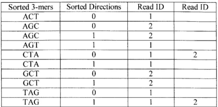
Table of k-m er Occurrences ... 102

Pairwise Read Alignm ents ... 103

Processing of Overlap Graph and Creation of Supercontig...104

Definition of Read "Shifts"...107

D iscarding Repetitive Links ... 108

Sparse Representation of Overlaps and Creation of Contigs...109

Assem bly of Contigs into Supercontigs ... Ill Results... 113

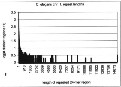
Repetition of k-m ers in the Test Sequences ... 114

Generation of Shotgun Data ... 120

Fragm ent Assembly Results ... 121

(5)

C h a p t e r 4 : Cross Species Genomic Comparison, and Gene Recognition...130

Introduction ... 130

Results... 132

Com parison of Hum an and M ouse G enom ic Loci ... 132

Global Sequence Alignm ent, GLASS ... 134

Gene Recognition, ROSETTA ... 137

Gene Recognition Results ... 139

M ethods...140

Database Construction... 140

Sequence Alignm ents and Com parative Analysis ... 141

Com putational Prediction of Coding Exons... 142

D iscussion ... 143

CON CLU SION ... 146

Appendix A : The G enetic Code ... 151

Appendix B: Perform ance of ARACHNE... 152

Appendix C: Comparative Analysis of Human and Mouse Loci...162

Appendix D: Combined Whole Genome Shotgun and Clone-by-Clone Assembly...176

(6)

LIST OF FIGURES

Number Page

BACKGROUND

0.1. T he G enetic C ode ... 17

0.2. Ambiguous and Unambiguous Read Overlaps...20

0.3. A Repeat Flanked by Unique Regions...23

0.4. Physical M apping ... 24

0.5. A Forw ard/R everse Link ... 27

0.6. Forward/Reverse Links Used in Fragment Assembly...28

0.7. Splicing and Translation... 32

0.8. Phylogeny Tree of M am mals... 35

Chapter 1: Physical Mapping with Repeated Probes 1.1. Gadget for Truth Assignm ent ... 47

Chapter 2: Sequencing a Genome by Walking with BAC-Ends 2.1. Overlapping BACs in Library of Depth d=12... 75

2.2. Serial Walking of the Genome from a Single Initial Seed Clone...77

2.3. Serial Walking of the Genome from a Collection of Seed Clones ... 78

2.4. Unidirectional Walking from a Seed Clone Co... . . . .. . . .. . . .. . . 79

2.5. Proportion of Excess Sequencing, One Library ... 82

2.6. Proportion of Ocean Excess Sequencing ... 83

2.7. N um ber of W alking Steps ... 84

2.8. Proportion of Excess Sequencing, Two Libraries...87

2.9. A Small Ocean Being Closed by Two Clones... 87

2.10. O ptim al Library D epth ... 88

2.11. Comparison of Parking and Exponential Distributions ... 91

2.12. Difference Between Parking and Exponential Distributions ... 93

2.13. Difference Between Formulas and Simulations ... 94

(7)

Chapter 3: Whole Genome Shotgun Assembly

3.1. Ambiguity Created by the Presence of Repeats...104

3.2. A R epeat w ith Three C opies... 105

3.3. A Sequence C ontig ... 106

3.4. Repetitive Links... 107

3.5. M erging of Supercontigs ... 113

3.6. 24-m er Frequencies in H. influenzae... 116

3.7. 24-m er Frequencies in A. fulgidus... 116

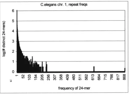
3.8. 24-mer Frequencies in C. elegans Chromosome 1 ... 117

3.9. 24-mer Frequencies in Human Chromosome 22...117

3.10. Repeat Lengths in H . influenzae... 118

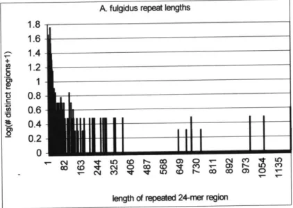
3.11. R epeat Lengths in A .fulgidus ... 118

3.12. Repeat Lengths in C. elegans Chromosome I...119

3.13. Repeat Lengths in Human Chromosome 22... 119

3.14. A Supercontig ... 122

3.15. Coverage of Genomes by Long Supercontigs ... 124

3.16. Quality of Shotgun Assembly on Human Chromosome 22...125

3.17. Quality of Shotgun Assembly on C. elegans Chromosome I...126

3.18. Quality of Shotgun Assembly on H. influenzae... 127

3.19. Quality of Shotgun Assembly on A. fulgidus ... 128

Chapter 4: Cross-Species Genomic Comparison and Gene Recognition 4.1. Correspondence of Regions on a Pair of Human/Mouse Homologous Loci ... 136

Appendix B: Performance of ARACHNE B. 1. Human Chromosome 22, 1x Coverage ... 154

B.2. Human Chromosome 22, 9x Coverage ... 154

B.6. C. elegans Chromosome 1, 11x Coverage ... 156

(8)

B .8. H . influenzae, I1x Coverage ... 157

B .9. H . influenzae, 9x C overage ... 158

B. 10. H influenzae, 7x Coverage ... 158

B .11. H influenzae, 5x C overage ... 159

B .12. A .fulgidus, 7x C overage...159

Appendix D: Whole Genome Assembly Using Combined Shotgun and Clone-by-Clone Sequencing (WGSCC Sequencing) B. 1. Coverage of the Genome with Shotgun and Clone-by-Clone Reads...154

(9)

LIST OF TABLES

Number Page

BACKGROUND

0.1. Genome Size and Number of Genes for Some Organisms...19

Chapter 1: Physical Mapping with Repeated Probes 1.1. Performance of GREED Y-MERGE-SPERNER on Simulated Data...71

Chapter 3: Whole Genome Shotgun Assembly 3.1. Exam ple of a Sorted H ash Table ... 102

3.2. Percentage of Genomic Sequence Covered by Unique k-mers...114

Chapter 4: Cross-Species Genomic Comparison and Gene Recognition 4.1. Training Set of Human/M ouse Homologs ... 138

Appendix A: The Genetic Code A .l. T he G enetic C ode ... ... 149

Appendix B: Performance of ARACHNE B. 1. Human Chromosom e 22, 11x Coverage ... 150

B .8. H . influenzae, IIx C overage ... 152

B .9. H . influenzae, 9x. C overage ... 152

(10)

B .11. H . influenzae, 5x C overage ... 153

B .12. A .fulgidus, 7x C overage...153

Appendix C: Comparative Analysis of Human and Mouse Loci

(11)

ACKNOWLEDGEMENTS

My most special thanks to my advisor Bonnie Berger for her guidance, unwavering support, and collaboration on all the work described in this thesis. I gratefully acknowledge the guidance and collaboration of Sorin Istrail, Eric Lander, and Jill Mesirov. Sorin Istrail introduced me to physical mapping, and Chapter 1 is the result of our collaboration. I feel especially fortunate to have met and collaborated with Eric Lander, who deeply influenced my work, my knowledge of biology, and my devotion to genomics research. Eric Lander introduced me to the material of Chapters 2, 3, and 4. These chapters resulted from my collaboration with Bonnie Berger, Eric Lander, and Jill Mesirov. I especially thank my friend and colleague Lior Pachter, whose contributions directly enabled the completion of the comparative sequence analysis and gene recognition part of this work (Chapter 4).

I thank Bruce Birren, Ken Dewar, Daniel Kleitman, and Tomas Lozano-Perez, for helpful discussions. I thank Eric Banks, Wes Beebee, Valentin Spitkovsky, Ken Stanley, Tina Tyan, Brian Walenz, and Bill Wallis, for help and contributions to the research. I am grateful to Angelita Mireles, Amir Nashat, and Ken Stanley for their help in reading over and helping edit my thesis. I thank my family, and especially my sister Evi, for their support. Thank you all.

(12)

(13)

OVERVIEW

The discovery of the DNA double helix in 1953 by James Watson and Francis Crick (Watson and Crick, 1953a, 1953b) led the way to an understanding of biology in molecular terms. Subsequently, since the discovery of techniques to sequence DNA in the late 1970s (Maxam et al. 1977; Sanger et al. 1977) the characterization and study of the genetic material of organisms at the sequence level has become an increasingly important tool in biology. Today major genomic projects are being undertaken at an accelerating pace, with the aim of sequencing and ultimately studying the genetic material of humans, animals, plants, bacteria, and in general a vast variety of living organisms. The Human Genome Project, an international effort to produce the complete sequence of human DNA at very high accuracy, is scheduled to complete by 2003 (Science, vol. 284, p. 1439). The mouse genome is next in the pipeline (Science, vol. 287, p. 1179). Organisms whose genome has already been sequenced include tens of unicellular organisms (see Hurowitz, 1999 for a list of 15 such organisms), yeast S. cerevisiae (Oliver et al. 1992; Dujon, 1996), C. elegans (The C. elegans sequencing consortium, 1998), and Drosophila (Nature, vol. 403, p. 817; Science, vol. 287, p. 1374). Many more organisms are either being sequenced, or will be sequenced in the near future. Finished sequences are being annotated with information about gene boundaries, regulatory elements, and other important biological units. Inter and intra-species comparative analyses of homologous regions are providing insight into the biology and evolution of organisms (O'Brien et al. 1999).

Since the first sequencing projects, computational tools have been essential in genomics. Shotgun sequencing for instance, the prevailing method for determining the sequence of a genomic region, involves obtaining a large number of short random pieces (a few hundred nucleotides long) of the region, sequencing those pieces with the existing sequencing technology, and then assembling them using computers into the complete sequence of the genomic region. As the pace of genomic research has been accelerating, the contribution of computer science is becoming both more essential and challenging.

(14)

In this thesis we will present some contributions of a computational/mathematical nature applied to the different stages of a genomic project. These stages include: planning a genome sequencing project, assembling the sequencing data into a complete genomic sequence, and finally comparing and annotating genomic sequences.

First, we will present theoretical work on the problem of finding the minimum superstring of a hypergraph. This is an algorithmic problem motivated by the biological problem of physical mapping, i.e. obtaining a map of the locations of clones for the purpose of then selectively sequencing them. We will study the computational complexity of this problem, and present some algorithms that provide constant approximations under certain conditions. We test our main algorithm on simulated random data.

Second, we will present a study of the "walking" approach to whole genome sequencing. Walking with clone-end sequences (Venter et al. 1996) is an important approach to genome sequencing, providing an alternative to either physical mapping-based clone-by-clone sequencing, or whole genome shotgun sequencing. We will present a mathematical model and computer simulations predicting the performance of a sequencing project based on walking with clone-end sequences. The purpose of our modeling work is to clarify important tradeoffs in planning to sequence a genome by this method. We also present a method for cutting dramatically the inefficiency of redundant sequencing, by using a second library of shorter clones.

Third, we will present some tools for automated assembly of shotgun sequencing data. We will present a hashing system for efficiently obtaining the adjacency matrix of similarity of a large collection of sequencing reads. Building on this, we will describe ARACHNE, a system for assembling shotgun sequencing reads into long layouts that we call supercontigs. We test a prototype implementation on the human chromosome 22, as well as on other sequences, with encouraging results. We briefly describe future improvements to ARACHNE, with the ultimate goal of having a system that can comfortably assemble shotgun data of a complete mammalian genome.

Finally, we will develop tools for comparison and annotation of large genomic regions of homologous DNA from two species. The impeding availability of vast amounts of unannotated human and mouse genomic data motivate this part of the work. The whole human genome will be available by 2003 while large regions of the mouse genome are being sequenced (Science, v. 284, p. 1906-1909, 1999; Science, v. 286, p. 210, 1999; Science, vol. 287, p. 1179, 2000) and in not

(15)

too long the complete mouse sequence will undoubtedly be obtained. The study of the human genome can benefit tremendously from comprehensive comparisons with the highly homologous mouse genome. Moreover, thinking ahead on future medical therapies and technologies based on genomics, they will likely be tested first on the mouse before being applied to the human. We will present GLASS (GLobal Alignment SyStem), a tool for aligning long orthologous genomic regions from related species. Using this, we will provide a comparative analysis of a number of orthologous genetic loci of human and mouse. Finally, we will present ROSETTA, a gene recognition program based on cross-species human and mouse genomic comparisons.

(16)

BACKGROUND

In the pages that follow we give a brief introduction to genomics, and outline the context of the contributions that we describe in the following chapters. We give basic biological background intended mainly for readers with expertise in computer science or related disciplines. Such readers may find it useful to also refer to more general texts such as (Lewin, 1996; Stryer, 1996; Lodish et al. 1998; Griffiths et al. 1993), and an introductory chapter on biology written for mathematicians (Lander and Waterman, 1995). For background more specific to the material in this thesis, we suggest the following selective reading: As general reading that is related to several parts of this thesis we would suggest Dujon, 1996; The C. elegans Sequencing Consortium, 1998; Lander, 1997; Lander and Waterman, 1988; Smit, 1995. For Chapter 1 on Physical Mapping, we would suggest Alizadeh et al. 1995; Booth and Lueker, 1976; Collins et al. 1995; Coulson et al. 1986; Greenberg and Istrail, 1995; Koop, 1995; Nelson and Speed, 1994. For Chapter 2, Venter et al. 1996; Lander and Waterman, 1988. For Chapter 3, Fleischmann, 1995; Green, 1997; Weber and Myers, 1997. For Chapter 4 we would suggest Altschul et al. 1990; Altschul et al. 1997; Batzoglou et al. 1998; Boguski et al. 1996; Burge, 1997; Burset and Guigo, 1996; Koop, 1995; O'Brien et al. 1999.

1. Genomes and the Genetic Code

DNA is a very long macromolecule composed of deoxyribonucleotides, which are small molecules containing a base, a sugar, and a phosphate group. The sugar contained in a deoxyribonucleotide is deoxyribose, indicating that it lacks an oxygen atom (deoxy-) that is present in a ribose. The base is a purine (adenine (A) or guanine (G)), or a pyrimidine (thymine (T) or cytosine (C)). Therefore DNA can also be thought of as a long string written in an alphabet of four letters, namely A, C, G, and T. DNA is actually a double-stranded molecule, where each nucleotide is bonded to its Watson/Crick complementary nucleotide (A to T, and C to G). Locally DNA assumes a helical shape, and therefore is called a double helix. James Watson and Francis Crick discovered the three-dimensional structure of DNA in 1953 (Watson and Crick, 1953a,b), and the mechanism of DNA replication was soon inferred. The complementary nucleotide chains

(17)

of DNA act as templates for each other during DNA replication. Therefore DNA is a large molecule containing information written in the alphabet {A, C, G, T}, capable of preserving and replicating this information. It is believed to contain (almost) all the information inherited by an organism from its parent(s).

The DNA of an organism is referred to as its genome. Genomes are stored inside cells. Organisms are broadly divided into prokaryotic organisms (or prokaryotes), and eukaryotic

organisms (or eukaryotes). The major difference is that the genome of eukaryotes is sequestered

in a nucleus, where it is protected by a nuclear membrane from the cytoplasm of a cell. The structure of the genome differs greatly between prokaryotes and eukaryotes, with eukaryotes usually having much longer genomes, exhibiting much higher repeat rates, and divided into a variable number of chromosomes. Multicellular organisms, i.e. organisms that have more than one cell, are usually eukaryotic. In multicellular eukaryotic organisms each cell has a nucleus with a copy of the DNA.

transcription translation

DNA - * mRNA p protein

Figure 0.1. The Genetic Dogma

The precise sequence of bases in the genome carries the genetic information of the organism. Genotype is the genetic constitution of an organism. Phenotype is the expression of this genetic constitution, i.e. the physical characteristics of the organism, and depends on the genotype and on the environment. Different organisms have genomes that are very different in size and structure. Viruses in general have the shortest DNA genomes' ranging from 5kb (kilo-bases) up to 200kb. Bacteria genomes are longer, ranging from 500kb to 5Mb (mega-bases) and circular.

(18)

The genome of yeast (a simple eukaryote) is 13.5Mb long (Sherman, 1997), contained in 16 pairs of chromosomes each ranging from 200kb to 2200kb in size.' The genome of the worm

Caenorhabditis elegans (or C. elegans) is 97.3Mb long and is contained in 6 chromosomes (The

C. elegans Sequencing Consortium, 1998). The genome of the fly Drosophila melanogaster is 165Mb long and is contained in 6 chromosomes (Rubin, 1996). The genome of a mammal such as human, or mouse, is believed to be around 3.5Gb (giga-bases) long. In some phyla, such as reptiles, birds, and mammals, genome sizes are similar within the phylum. But in the case of insects, amphibians, and plants, genomes vary widely in size within a phylum. Flowering plants have the greatest variation in genome sizes, ranging from smaller than 100Mb, to greater than 100Gb (Lewin, 1996).

Cells make proteins, which are the building blocks of a living organism. Proteins are synthesized according to the information encoded in genes, which lie in the genome. The expression of the information in a genome thus takes the following steps: genes are initially

transcribed into messenger RNA (mRNA), which is an information-carrying intermediate in the

protein synthesis mechanism. Messenger RNA in turn is translated into protein. A schematic is shown in Figure 0.0.1. RNA molecules are usually single-stranded, and are composed of adenine (A), cytosine (C), guanine (G), and uracil (U) instead of thymine (T). An mRNA transcript contains a single gene in eukaryotes, but in prokaryotes it usually contains multiple genes. Translation to protein takes place according to the genetic code, whereby three nucleotides are translated to one amino acid, which is a unit in a protein sequence, just like nucleotides are units in DNA and RNA sequences. There are 20 amino acids. Therefore the genetic code is redundant, as there exist 64 combinations of triplets of nucleotides. Three such combinations actually stand for the special terminator signals of translation, the stop codons: UAA (ochre), UAG (amber), and UGA (opal). One triplet (AUG) stands for the initiation of translation signal, as well as for the amino acid Methionine (Met). The full genetic code appears in Appendix A. Later in this section we give more details on the structure of the gene and on the processes of transcription and translation.

We omit from this simple picture the fact that some of the DNA of an organism, and specifically yeast. is contained in mitochondria, plasmids, and even some double-stranded RNA viruses.

(19)

The human genome is believed to contain up to 100,000 genes. Probably by the end of the year this estimate will be more accurate, as human genome projects approach their conclusion. Other mammalian genomes are believed to contain a similar number of genes. Genes in other organisms vary. Table 0.1 shows estimated lengths of genomes and number of genes for a number of organisms (Meinke et al. 1998; O'Brien et al. 1999; Rubin, 1996; Lewin, 1996; The C. elegans Sequencing Consortium, 1998, Lin et al. 1999, Adams et al. 2000).

Organism Length (Mbp) Number of Genes

Human (and other mammals) 3,500 70,000-100,000

Drosophila (fruit fly) 120 13,600

Caenorhabditis Elegans (nematode) 97 19,000

Saccharomyces Cerevisiae (yeast) 13.5 5,800

Haemophilus Influenzae (bacterium) 1.83 1,738

Escherichia Coli (bacterium) 4.2 2,350

Arabidopsis Thaliana (plant) 120 27,000

Table 0.1. Estimated genome size and number of genes for some organisms.

2. Mapping and Sequencing a Genome

The complete DNA sequence of a genome is a powerful tool for studying an organism. Biological research in the 21st century will surely require obtaining the sequence of large numbers of important organisms, including many higher animals and plants with large genomes. Obtaining the genome sequences of living organisms is widely considered to be the first step towards a deeper understanding of genetics and biology in general. There is no simple biological experiment that can sequence an entire genome. There are several experiments though, that combined give much of the desired answer.

The first procedures that were able to determine the nucleotide sequence of small fragments of DNA emerged in the late 1970s (Maxam et al. 1977; Sanger et al. 1977). These procedures involved gel electrophoresis, an important biological experimental method. We refer the reader to standard introductory biology and biochemistry books (eg. Lodish et al. 1996). This is still the predominant method for sequencing DNA fragments. It can produce the sequence of a

(20)

500-1000 nucleotide long region off the end of a DNA fragment. The gel electrophoresis reaction is error prone, yielding around 1% incorrect nucleotides in the first 500 positions, and somewhat higher error rates in the subsequent positions. In addition, it is not possible to tell which of the two complementary strands of DNA is given by the reaction. The output of the experiment is called a read, and as we said is a 500-1000 long sequence on {A, C, G, T} of unknown orientation, and with -% errors.

A. A<k read 2 read 1 A>k B. read 4 OK read 3

Figure 0.0.2. Ambiguous and unambiguous read overlaps. For the value of k, A. Reads 1 and 2 overlap by less than k, and therefore the overlap is ambiguous; B. Reads 3 and 4 overlap by more than k, and therefore

are very likely to truly overlap in the genome.

The predominant method for characterizing longer regions is called shotgun sequencing, and was developed by Sanger's lab in 1982 (Sanger et al. 1982). The method involves (1) breaking several replicas of the DNA region of interest into many smaller pieces, at random; (2) obtaining reads using gel electrophoresis for a large number of those pieces; (3) finally detecting overlaps between the reads, and assembling them together using computers (in silico). In order for this approach to work, during step 2 a sufficient number of reads should be obtained. The

(21)

coverage with reads of a region of length L is defined to be C, where CxL is the sum of lengths

of reads obtained in step 2. In such sequencing experiments, typical coverage values are 5-10, with coverage 10 being considered the "golden" quality standard.

Sanger's lab first applied shotgun sequencing to the genome of bacteriophage A (Sanger et al. 1980, 1982). Subsequently genomes of large recombinant plasmids, large viruses, mitochondria, chloroplasts and bacteria were sequenced by this technique (Goebel et al. 1990; Oda et al. 1992; Ohyama et al. 1986; Fleischmann et al. 1995).

Fragment assembly is the computational problem of figuring out the source genomic

sequence, given a collection of reads obtained by shotgun sequencing. In the absence of sequencing errors and repeats, fragment assembly is a trivial computational task, given a sufficiently large number of sufficiently long reads. Some back-of-the-envelope analysis demonstrates this claim. Let G be the genome length, N the number of reads, and assume for simplicity a constant read length 1. Assume that the genome is a random string on {A, C, G, T}, with each letter occurring with probability 4- at each position independently of other positions. The probability that a given substring of length k (call it a k-mer) occurs in the genome is

4-kxG. _{The probability it occurs twice is} _4-2kxG2

. There are 4k k-mers, therefore the probability that any occurs twice in the genome is 4-xG2

.Letting k= Flog4G2 + log4103] the probability

that there is a repeated k-mer is 10-3, which is very small. For G = 3.5x 109, roughly the length of the human genome, it would suffice for k to be > 37 in order to virtually ensure that two reads containing the same k-mer correspond to overlapping subsequences in the genome. This is shown in Figure 0.0.2. Then a simple algorithm would suffice to produce in linear time an assembly of the reads into large contigs: (1) create a hash table of all k-mers occurring in the reads, indexing the reads; (2) perform in any order, all possible pairwise "merges" of reads that contain a common k-mer. Step 1 above is linear in CxG, while step 2 is linear in CxN.

Factors that make fragment assembly considerably more challenging are (1) sequencing errors that result in reads with slightly different sequences in the region of overlap, and (2) the repetitive structure of genomes, especially for higher organisms and longer genomes. Currently

PHRAP (PHragment Assembly Program, or Phil's Assembly Program after Phil Green,

(22)

shotgun data. It has been used successfully in most sequencing efforts in academia. It can handle routinely shotgun data of Bacterial Artificial Chromosome (BAC)' clones, which are usually 100-300Kbp long. It is believed to be capable of handling shotgun data of sequences that are at most a few million base pairs long, such as bacterial genomes (Lander, personal communication).

The major challenge when assembling shotgun data from large genomic regions is the presence of repeats in the genome. Different genomes exhibit different amounts and kinds of repetition. Bacterial genomes usually have very few repeats. Eukaryotic genomes usually exhibit a considerable amount of repetition. Low complexity repeats are regions of DNA that are extremely high in purines (A and T), or pyrimidines (C and G), or A and C, or G and T, or regions that contain microsatellite repeats,2 or simply regions that are extremely rich in a particular nucleotide. Such regions clearly deviate considerably from a random sequence on {A, C, G, T}. In addition, there are common families of repeats. One example, Alu, are small repeats of length around 300 that tend to cluster, and are around 10% different between copies (Schmid, 1996; Batzer et al. 1996). LINEs (Long Interspersed Nucleotide Elements) are another family of repeats, of length between 500 and several thousand nucleotides (Smit and Riggs, 1995). The human genome contains roughly 1,000,000 Alu occurrences, and 200,000 LINE occurrences. Many other repeat families have been identified, including MIR and LTR/Retroviral (for a comprehensive review see Smit, 1995). Finally, possibly 25% of the genes in the human genome are repeated twice or three times within the genome, and there are also 43kb long tandem clusters of RNA pseudogene arrays, and 50-150kb long genome duplications (Myers, 1999). Such repetitions exhibit different degrees of fidelity between copies.

'Bacterial Artificial Chromosomes are a vector mechanism that can accommodate contiguous pieces of DNA that are fairly long (up to 300,000 long in general). Other vector mechanisms include plasmids, cosmids, Phage artificial chromosomes (PACs), and Yeast Artificial Chromosomes. Cloning of DNA is based on two key types of enzymes:

restriction enzymes that are capable of cutting the DNA from any genome at occurrences of specific short subsequences

of nucleotides, generating a well-defined set of fragments; and DNA ligases, capable of inserting the DNA fragments produced by restriction enzymes into replicating DNA molecules. Such replicating DNA molecules (vectors) include

plasmids (often E-Coli plasmids) that can incorporate fairly short DNA sequences, on the order of 2,000-12,000

nucleotides long, cosmids that can incorporate longer sequences, on the order of ~40,000 long, Bacterial Artificial

Chromosomes (BA Cs) that incorporate longer sequences of around 150kb long, and Yeast Artificial Chromosomes, that

incorporate much longer sequences, on the order of 1Mb long. Different vector clone mechanisms exhibit various "hot" and "cold" spots in the genome, i.e. subregions of the genome that tend to be incorporated more frequently, or less frequently. The reason is restriction enzymes cut DNA in the occurrences of specific short sequences. This process is not entirely random, as DNA sequence does not obey much of the properties of a random string on four characters.

2 _{Repeats of the form (al.. .ak) where 3 k 6 and n is a very large number. The subsequence al.. .ak is repeated n}

(23)

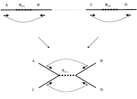
In the presence of repeats, overlaps between pairs of reads do not unambiguously imply that the reads truly overlap in the genome. Figure 0.0.3 demonstrates how a repetition in the genome makes it hard to assemble the corresponding regions.

A R B C R(2) x a b D c d a A x y C C R _b B d D

Figure 0.0.3. (Above) Repeat region R is flanked by unique regions A, B (R 1) occurrence) and C, D (R2) occurrence). Reads x, y are completely inside the repeat occurrences, while reads a, b, c, and d are partially in the repeat, and partially in the unique regions. (Below) Correct assembly of the reads is a-x-b and c-y-d. However, wrong assemblies c-x-y-b, c-x-b, c-x-d, a-x-y-d, etc. are all consistent with the overlap picture.

Largely because of the presence of repeats, until recently it was widely believed that sequencing a large, repeat-rich genome with the shotgun approach and then accurately assembling the sequence is not feasible. For this reason, clone-by-clone approaches to sequencing a genome have been employed. According to these approaches, subsequences of the genome are inserted into vectors that can accommodate them, creating clones that can be reliably replicated. Enough clones are created to cover the whole genome with redundancy. Shotgun sequencing is

(24)

then applied to a subset of clones that has been selected so as to cover the entire genome with minimal redundancy. These approaches overcome the challenges of sequencing an entire repeat-rich genome using the shotgun method. Applying shotgun sequencing to each individual clone is much easier because (1) the subsequence is much shorter and consequently the computerized assembly of reads much smaller, and (2) a clone has a much simpler repetitive structure than the whole genome.

A chromosome

Physical Mapping

Minimal tiling path: Sequencing

Figure 0.0.4. Clones, possibly from different kinds of vectors and of different sizes cover the chromosome. The clones are mapped so that their layout on the chromosome is known accurately enough to construct a tiling path. The clones in the tiling path are selected so as to minimize overlaps, while not allowing any

gaps. These clones are eventually sequenced, providing the sequence of the chromosome.

Physical mapping is the predominant clone-by-clone approach to-date. (Other approaches have been proposed, see for instance Hudson et al. 1995; Venter et al. 1996; Batzoglou et al. 1999, and Chapter 2). According to this approach, as a first stage of a sequencing project, a large

(25)

library of clones is constructed covering the entire genome. The clones are mapped on the genome, i.e. their layout is known. Subsequently, a minimal tiling path of the clones is selected for the sequencing pipeline. Figure 0.0.4 shows an example of a mapped set of clones and a tiling path, for one contiguous piece of DNA (e.g. a chromosome). Note that in reality the DNA of a chromosome cannot be conveniently isolated. Therefore one cannot select and clone a random fragment off a specific chromosome. In order to sequence clones from a specific chromosome, the clones need to be mapped first to the chromosome.

The physical mapping techniques can be divided in two categories: digestion experiments,

and hybridization experiments.

In digestion experiments a collection of clones is cut (digested) using one or more restriction enzymes, that each split the inserts at every occurrence of a characteristic substring of 4-8 nucleotides. Then the lengths of the resulting insert fragments are determined (usually using gel electrophoresis). Pairs of clones that exhibit similarities in the pattern of resulting fragment lengths are considered likely to overlap in the genome. Variations in the digestion technique include (1) single digests, in which one restriction enzyme is used; (2) double digests, in which two restriction enzymes are used, each cutting the inserts at occurrences of a different substring; (3) partial digests, where the target DNA is cut by one enzyme, but the experiment is performed multiple times, varying the duration of enzyme activity on each copy of the inserts. By varying the time the enzyme acts on DNA, larger or smaller sets of sites are recognized and cut by the enzyme.

In hybridization experiments, the presence or absence of a set of oligonucleotide probes is used to determine overlaps between insert clones. Oligonucleotide probes are small sequences of DNA that bind (hybridize) to their Watson/Crick complementary subsequences on a single-stranded insert clone. Probes detect overlap because when a set of probes hybridizes to the same pair of clones, the corresponding set of subsequences occurs in both clones. Hybridization experiments can be performed with simple oligonucleotide probes, or with STS probes. The STS

(26)

probes are pairs of 18 long substrings that are between 200 and 1,000 nucleotides apart in the insert. A region containing such a pair is called a Sequence Tagged Site (STS).'

Several kinds of experimental errors may occur with any of the above physical mapping techniques. In digestion experiments, typical errors include uncertainty in length measurements, multiplicity errors where the number of fragments of same lengths is miscounted, spurious or missing fragments, and other. Gel electrophoresis data on the lengths has typical error rates of 3% (Fasulo et al. 1997). In hybridization experiments, typical errors include repeated probes,

chimeric clones, false positives, andfalse negatives (Greenberg and Istrail, 1995, Batzoglou and

Istrail, 1999, Myers, 1999, see also Chapter 1). A false positive is the hybridization of a probe to a clone where it does not occur. A false negative is the absence of hybridization of a probe to a clone where it occurs. A chimeric clone is a piece of DNA coming from two different parts of the genome glued and appearing contiguous. A repeated probe is a probe that occurs at least twice on the mapped region, wrongly implying overlap between clones covering two different occurrences

of the probe.

A fundamental question when constructing physical maps is to determine the number of clones needed to cover a genome. Lander and Waterman (1988) introduced a statistical model for answering this and related questions. Clones in the Lander-Waterman model are intervals of length L, each uniformly distributed along the genome which is a large interval [0,N] of length N. Clones cover the genome to depth (coverage) d = nL/N where n is the number of clones. The expected number of gaps in the genome (subregions not covered by any clone) is found to be ne" + 0(1), and the expected total gap length2 is found to be Ne-d.

Whole-genome shotgun sequencing is an alternative to the clone-by-clone approaches. An important variation of the technique, that considerably facilitates fragment assembly, is shotgun sequencing with forward-reverse links (Edwards and Caskey, 1991). According to this technique, reads are obtained from both ends of an insert (Figure 0.0.5). Moreover, inserts are size-selected so that the approximate distance of the pair of reads obtained from the ends of a fragment is

'STS probes are currently more popular because they are a more reliable and efficient means of obtaining the overlap information between clones (Myers, 1999).

2 For the Human Genome, letting N = _{3,500Mb, and given a library of n = 175,000 BAC clones of length around}

(27)

known. Plasmid inserts for instance, can be size selected to be approximately L long, with 2,000 < L < 12,000. One of the reads is always obtained by reading the forward strand of the fragment, and the other by reading the reverse complement strand. This is why the link between the reads is

called a reverse link. Because of imperfection in the experimental methods, forward-reverse links are inaccurate in two ways: (1) some links, typically 10% (Myers, 1999) are false with the respective reads coming from unrelated places in the genome; (2) distances between the reads are only approximate, with typical mean deviations in the 5-10% range. For simplicity we will also refer to forward-reverse links as earmuff links, or earmuffs.

Approximate distance L ± 10%L

read I read 2

Insert, size selected for length L

vector

... Insert -- Reads

Q

_") Vector _{Forward/Reverse link}

Figure 0.0.5. A forward/reverse link is obtained by reading off both ends of an insert.

Forward/reverse links can provide crucial information that aids in resolving repeats in the genome. Recall Figure 0.0.4, where regions A and B flank occurrence I of repeat R, and regions C, D flank occurrence 2 of R. Without any forward/reverse link information, it may not be

(28)

possible to deduce that A-R-B, C-R-D is the correct sequence, as opposed to A-R-D, C-R-B. Figure 0.0.6 shows how forward/reverse links can resolve the ambiguity.

A R1 B C R(2) D

A B

Ro

C D

Figure 0.0.6. Forward reverse links between regions A,B, and C,D, resolve the ambiguity in the assembly. It is clear using the link information that regions A and B flank one copy of R, while regions C and D flank

another copy of R.

Shortly after sequencing of an entire mammal genome became a realistic possibility, the US National Institute of Health, and the Department of Energy in collaboration with UK's Sanger center and other labs in Europe and Japan, announced the launch of the Human Genome Project (HGP) in 1990. A timetable was set for initially mapping, and subsequently sequencing the human genome with an objective to complete the project by 2005 (Collins and Galas, 1993). Subsequently, new goals were set for the HGP to complete by 2003, while also providing 90% of

(29)

the genome in a working draft by the end of 2001 (Collins et al. 1998). The HGP set a quality standard for finished sequence, of 99.99% - less than one error per 10,000 bases.

The Human Genome Project has been following the clone-by-clone approach. Weber and Myers (1996) proposed that the approach be shifted, to whole-genome shotgun sequencing. They provided a computer simulation demonstrating the feasibility of this approach. Their arguments in favor of shotgun sequencing included (1) better speed and cost; (2) detection of DNA polymorphisms;' (3) more complete coverage of the genome. Most notably they argued that pure shotgun sequencing could be performed in a centralized, efficient way, cutting the costs of the key procedures in a large factory setting. It would also avoid various steps needed in the clone-by-clone approaches, such as generation, storage, and tracking of large insert clones and smaller subclones. Finally it would avoid inefficient overlaps between clones that are being sent to the sequencing pipeline. On the other hand, Green (1996) advised against whole genome shotgun sequencing. The main argument against the shotgun method was the risk involved with performing all the costly sequencing work at once, and afterwards trying to assemble everything on a computer. Green (1996) argued that this approach may not yield a correct result, or a verifiable result, it may yield large-scale misassemblies of the sequence that are hard to detect and correct, and the finishing phase may prove more costly than the savings from previous phases.

In the past few years there has been a debate as to the strengths and weaknesses of each sequencing approach, mostly in view of the impending completion of the Human Genome Project. A privately owned company, Celera, in collaboration with academic partners, has been able to sequence the Drosophila genome by the shotgun approach combined with sequence obtained in the more traditional ways (Science, vol. 287, p. 767). Celera will partially sequence the human genome with shotgun, and combine the data with those of the Human Genome Project (Science, vol. 287, p. 1179). The few coming years will settle the debate regarding the efficiency and reliability of the various approaches for sequencing a large genome. Perhaps the optimal approach will prove to be a hybrid method of whole-genome shotgun sequencing using various vectors (yielding forward/reverse links of different lengths) and light shotgun sequencing of large inserts that cover the genome to some low depth (Lander, personal communication). The idea of

(30)

this approach would be to provide much of the needed sequencing through the whole-genome shotgun method, while using the light sequencing of random large clones as powerful additional linking information. The Drosophila genome was obtained with a hybrid method and Celera plans to obtain the Human Genome with a hybrid method. Finally, the mouse genome is in the pipeline to be sequenced by the academic sequencing community using a hybrid shotgun/clone-by-clone method (Science, vol. 287, p. 1179). The optimal combination of shotgun/hybrid for a large mammal genome is a very important open question (Lander, personal communication).

3. Genome Annotation

DNA is encoded into proteins according to the processes of transcription and translation (the Genetic Dogma). Not all of the DNA sequence is coding. In fact in mammals only a small percentage of the genome is coding. Segments of the genome that are translated comprise 75% of the yeast genome; they represent only about 3% of the human genome. One of the first steps

in studying a genomic sequence is to identify the coding regions, and predict the encoded proteins. Given that transcription and translation are highly regulated processes, it is also useful to detect the precise locations of regulatory elements and other relevant subsequences that

affect the processes of transcription and translation.

Before we discuss genomic annotation, we need to give a brief description of the processes of transcription and splicing. In the discussion that follows we will focus on eukaryotic organisms, and more specifically on mammals. In general bacteria do not have splicing, while the lower eukaryotes exhibit splicing to a lesser extent than higher ones.

RNA polymerase performs transcription by copying the DNA strand into an RNA strand

that grows from 5' to 3'.' The copying is accomplished according to the rules of Watson-Crick base pairing. The source DNA is said to act as a template for copying into the newly formed RNA strand. The resulting RNA strand has the reverse complement sequence of the template. The RNA polymerase interacts with specific promoter sequences that are upstream of the

DNA and RNA single stranded molecule ends are named 5' or 3' after the orientation of the 5' and 3' carbon atoms of the sugar ring. All known RNA polymerases synthesize chains directionally from 5' to 3'.

(31)

template and indicate the location where transcription should start. There are several kinds of promoter consensus sequences but in general there is no satisfactory computational method of recognizing promoters. Transcription is a most essential biological process, and its regulation is extremely important. Different organisms have various methods of regulating transcription. In addition to the promoter sequences, enhancer sequences can also regulate transcription. Enhancer sites are located at various distances from the transcription start; proteins bind at these sites and contribute to the regulation of RNA polymerase activity. Identification and annotation of these regulatory sequences by computational methods is a very important open problem. It would be a first step in understanding the mechanisms of regulation of specific genes.

Splicing occurs in RNA after transcription, and before translation. RNA before splicing is

called pre-mRNA, while after splicing it is called mRNA. During splicing, certain enzymes (the spliceosomes) act upon pre-mRNA to delete certain segments called introns and connect together

the remaining segments, called exons. The resulting sequence is used in translation, while the introns are thrown away.' Translation is executed by the ribosome, a large RNA/protein complex, and starts at an occurrence of the triplet AUG.2 The translation start is usually surrounded by a weak consensus sequence, known as the Kozak consensus.3 Translation proceeds directionally

5'-> 3'. Each triplet of nucleotides (called a codon) after the translation start is translated into an

amino acid, according to the genetic code (Appendix A). This defines the coding frame of the gene. Translation stops at the first occurrence of a stop codon in the coding frame, which is as UAA, UAG, or UGA. Therefore, the translated part of the sequence contains no triplets UAA, UAG, or UGA in the coding frame. The leftmost untranslated part of the sequence, before the initiating AUG, is called the 5' untranslated region (5'-UTR), and the rightmost untranslated part, after the stop codon, is called the 3' untranslated region (3'-UTR). Abusing terminology, we will call the post-spliced segments coding exons or noncoding exons, depending on whether they are translated, or untranslated. Thus an exon may be fully coding, fully noncoding, or it may consist of a coding exon and a noncoding exon. A schematic is given in Figure 0.0.7. Three introns are

' Virtually all mRNA in vertebrate and insects are derived by splicing of pre-mRNA as described above. However, in some protozoans as well as in around 10-15% of the genes of the worm Caenorhabditis Elegans, a process of trans-splicing takes place whereby mRNA is produced by trans-splicing together different RNA molecules (see Lodish, 1998).

2 _{In humans the codons AUA and AUU also appear as initiation codons, while in mice AUC is also used. These} occurrences are extremely rare and are usually ignored in computational recognition of genes.

(32)

spliced, generating 4 exons. In our terminology we have two 5' noncoding exons, three coding exons, and one 3' noncoding exon. The 5'-UTR for example, consists of the first exon and part of the second exon. In our terminology it consists of the first two noncoding exons.

Splicing of introns is controlled by the consensus sequence around the splice sites, which are the boundaries between introns and exons. The splice site at the 5' end of an intron is called

the donor splice site, and the splice site at the 3' of an intron is called the acceptor splice site.

Exon 1 Exon 2 Exon 3 Exon 4

Intron Intron 2 Intron 3A

pre-mRNA 3' Splicin mKNA Translation Introns

--ME Noncoding Exons Coding Exons

AUG -

E1.X

STOP

protein sequence protein 3D structure

Figure 0.7. Splicing and translation. The pre-mRNA transcript undergoes splicing, where long segments (introns) are removed and the rest (exons) are glued together into the mRNA transcript. This in turn undergoes translation, where each triplet of codons after the first AUG is translated into an amino acid

according to the genetic code, resulting in a protein sequence (XI.. .Xn). This in turn is folded into a functional three-dimensional structure.

.

..

(33)

The donor splice site is generally characterized by a strong consensus of GGURAGU where R stands for either A or G. The above consensus runs from the last position of the upstream exon, up to the 6th position of the intron. Less than half the splice sites obey the above

consensus. However, the first two positions of an intron are GU in the vast majority of the introns.' Even though the few nucleotides adjacent to the GU start of an intron seem to be the most important in determining the splicing reaction, the region up to 20 base pairs into the intron seems to also play an important role. In certain introns, occurrences of GGG in that region play an important role in splicing (McCullough and Berget, 1997).

The acceptor splice site exhibits a weaker consensus of CAGR, where AG is always the 3' end of the intron.2 Usually inside the intron and upstream of the acceptor splice site, lies a pyrimidine-rich region of length around 20, known as the pyrimidine tract. Further upstream often lies a branch site, which has the biological role of attaching to the 5'-end of the intron during splicing. The branch site lies usually immediately upstream of the pyrimidine tract. In yeast the branch site has a strong consensus of UACUAAC where the highlighted A is the point where the 5' end of the intron attaches, called the branch point. In human DNA there is a much weaker consensus of YNYURAY (Y stands for C or T, and N stands for any nucleotide).

Splicing is in general deterministic: for the majority of the genes, it is believed that the same genomic region always produces the same mRNA and protein products. However several genes can be spliced into a number of different variants depending on the environment or on the developmental stage of the organism. Those are called alternatively spliced genes, and the different splice sites that are used are called alternative splice sites.

The above discussion focused on the splicing of the vast majority of introns in pre-mRNA of insects and vertebrate. A different kind of splicing is exhibited in group I and group II introns. Group I introns are prevalent in nuclear ribosomal RNA (rRNA) genes of protozoans. Group II introns are found in organelles such as mitochondria and chloroplasts from plants and fungi. Group I and II introns exhibit self-splicing mechanisms where a spliceosome is not employed, and the RNA product catalyzes its own splicing reaction. The consensus sequences at the ends of

GC is also observed in some cases.

(34)

introns are vastly different for these groups of introns. We refer the reader to (Cech, 1990; Phizicky and Greer, 1993; Lodishet al. 1998) for further discussion on the splicing of group I, II introns, as well as to (Sharp and Burge, 1997) for splicing of some introns using a different spliceosome. A theory is that spliceosome-based splicing evolved from self-splicing reactions (Lodish et al. 1998).

Annotation of genomic sequence involves identification of the genes encoded in the sequence, including the boundaries of the regions that act as templates for transcription, the initiator and terminator of translation, splice sites, promoter and regulatory regions, and perhaps several other biologically important elements. Experimental methods exist for the accurate identification of most of the above elements, but it is generally understood that these methods are expensive, and too slow for the accelerating speed with which genomic sequence is being produced. For this reason computational methods play an essential part in genomic annotation. The identification of boundaries of coding exons, usually referred to as exon prediction, or gene

recognition, is one of the most active areas of research in computational genomic annotation.

Unfortunately computational methods are usually not as accurate as experimental methods, and computer-derived annotations often need to be experimentally verified.

Following annotation of sequence, a very important step in the study of a genome is functional annotation. Functional annotation is the process of assigning function to the genes that are expressed in the genome, discovering the mechanisms of regulation associated with different regulatory sites, and more generally assigning function to structural elements annotated in the genome. This step is very challenging and currently lags behind the sequencing and structural annotation steps (O'Brien et al. 1999).

4. Comparative Genomics

Genomes of different organisms exhibit similarities largely because of evolution from a common genome. For instance, the first mammal lived around 165 million years (Myr) ago. All modern mammals have a common ancestor that is dated between 65 Myr ago and 100-120 Myr ago. A common primate ancestor is believed to have lived around 60 Myr ago (O'Brien et al. 1999). Figure 0.8 shows the phylogeny tree for different well-known mammal orders (the more complete tree can be found in http://Ag.Arizona.Edu/tree/).

(35)

Edentata (anteaters, sloths,

armadillos)

New World monkeys

Old World monkeys Lagomorpha

(rabbits) humans, gorilla,

Triconodonts Rodentia (mice, bhimpanzee,

rats, squirrels)

Mammals Multitubereulata Primnates

gibbons

Monotremata Tree shrews

(platypus,

eehidnas) Bats lemurs,

galagos,

Eutheria lorises

(plaeental Colugos

animals)

Artiodactyla (pigs, deer, eattle, Marsupialia goats, sheep, hippopotaunuses,_{camels, etc.)}

(opossinns, _{Cetacea (whales, dolphins, porpoises)}

kangaroos)

Perissodactyla (horses, tapirs, rhinoceroses)

Proboseidea (elephants, amnmoths) Carnivora (dogs, eats,

bears, raccons, weasels, mongooses, hyenas)

Figure 0.8. Part of the evolutionary tree for mammals. Refer to http://Ag.Ariziona.Edu/tree/ for a fuller version of the tree of life.

Genomes change from generation to generation, by many different processes. The most local process is the random introduction of isolated mutations in the genome sequence that involve either base substitutions (change of a base pair among {AT, CG, GC, TA} to another), or insertions/deletions of a particular base pair (indels). Such mutations can be silent if they have no expressed effect (no effect in the phenotype) such as when a mutation occurs in an intron whose precise sequence presumably does not have any effect on the characteristics of the organism, or when a mutation occurs in the third position of a codon in an exon and does not change the encoded amino acid (refer to Appendix A). Other mutations change one amino acid but do not have any effect in the resulting protein activity (neutral substitutions). Point mutations are base