Computational Experiments for Local Search
Algorithms for Binary and Mixed Integer
Optimization
by
Jingting Zhou
B.E. Biomedical Engineering, Zhejiang University, 2009
Submitted to the School of Engineering
in partial fulfillment of the requirements for the degree of
Master of Science in Computation for Design and Optimization
at the
MASSACHUSETTS INSTITUTE OF TECHNOLOGY
ASSACHUSETTS INSTITUTE OF TECHNOLOGY
SEP 0 2 2010
LrB1RARIES
ARCHIVES
September 2010
@
Massachusetts Institute of Technology 2010. All rights reserved.
Author ...
!..
... J...
School of Engineering
August 4, 2010
C ertified by ...
...
...
Dimitris J. Bertsimas
Boeing Professor of Operations Research
Thesis Supervisor
Accepted by ...
'......6"
Karen Willcox
Associate Professor of Aeronautics and Astronautics
Codirector, Computation for Design and Optimization Program
Computational Experiments for Local Search Algorithms for
Binary and Mixed Integer Optimization
by
Jingting Zhou
Submitted to the School of Engineering on August 4, 2010, in partial fulfillment of the
requirements for the degree of
Master of Science in Computation for Design and Optimization
Abstract
In this thesis, we implement and test two algorithms for binary optimization and mixed integer optimization, respectively. We fine tune the parameters of these two algorithms and achieve satisfactory performance. We also compare our algorithms with CPLEX on large amount of fairly large-size instances. Based on the experimental results, our binary optimization algorithm delivers performance that is strictly better than CPLEX on instances with moderately dense constraint matrices, while for sparse instances, our algorithm delivers performance that is comparable to CPLEX. Our mixed integer optimization algorithm outperforms CPLEX most of the time when the constraint matrices are moderately dense, while for sparse instances, it yields results that are close to CPLEX, and the largest gap relative to the result given by CPLEX is around 5%. Our findings show that these two algorithms, especially the binary optimization algorithm, have practical promise in solving large, dense instances of both set covering and set packing problems.
Thesis Supervisor: Dimitris J. Bertsimas Title: Boeing Professor of Operations Research
Acknowledgments
After hundreds of hours' effort, I have fulfilled my thesis at MIT. It is an absolutely tough and challenging task. And without the following people for their help, I couldn't achieve my goal eventually.
First and foremost, I would like to express my deepest gratitude to my supervi-sor, Professor Dimitris Bertsimas, for his invaluable guidance through my thesis. I expecially appreciate the time he devoted to guide me, his insightful opinions, and his encouragement to cheer me up in face of difficulties. He has also set a role model to me, for his endless passion on work and great dedication to operations research.
My gratitude extends to Dan Iancu and Vineet Goyal, who have given me enor-mous support in my project. They are always very responsive to my inquiries and willing to spend time with me discussing my project. I am also touched by the friend-liness of people at ORC, Andy, Michael and Bill, without their help, I couldn't keep my project going so smoothly.
I have enjoyed a great time at MIT for the past year, all because of you, my beloved SMA friends. The trip to Orlando, the gatherings at Mulan, we have spent so many fun moments together. I have also enjoyed so much the chat with Gil, Jamin, Wombi and Joel. They have shown great support to my work as the representative of CDO at GSC.
I would also like to thank SMA for providing a fellowship to support my study at MIT, and the staff at the MIT CDO office and SMA office who have made this period in Boston one of the greatest memory in my life.
Last but not least, I owe my deepest thanks to my parents for their unconditional love and belief in me. My love for them is more than words that I can say.
Contents
1 Introduction
2 A General Purpose Local Search Algorithm for Binary Optimization 2.1 Problem Definition ...
2.2 Algorithm ... ... ... 2.3 Implementation Details ... ... 2.4 Computational Experiments ... ... 3 An Adaptive Local Search Algorithm for Mixed Integer
tion 3.1 Problem Definition ... 3.2 Algorithm... . . . . 3.3 Implementation Details... . . . .. 3.4 Computational Experiments... . . . . Optimiza-4 Conclusions
List of Tables
2.1 Characteristics of set covering instances for IP . . . . 23
2.2 Computational results on set covering instances 1.1-1.10 . . . . 23
2.3 Computational results on set covering instances 2.1-2.10 . . . . 24
2.4 Computational results on set covering instances 3.1-3.10 . . . . 24
2.5 Computational results on set covering instances 4.1-4.10 . . . . 25
2.6 Computational results on set covering instances 5.1-5.10 . . . . 25
2.7 Computational results on set covering instances 6.1-6.10 . . . . 26
2.8 Computational results using running sequence II . . . . 27
2.9 Characteristics of set packing instances for IP . . . . 28
2.10 CPLEX performance with different MIP emphasis settings . . . . 29
2.11 Computational results on set packing instances 1.1-1.5 . . . . 29
2.12 Computational results on set packing instances 2.1-2.5 . . . . 30
2.13 Computational results on set packing instances 3.1-3.5 . . . . 30
2.14 Computational results on set packing instances 4.1-4.5 . . . . 30
2.15 Computational results on set packing instances 5.1-5.5 . . . . 31
2.16 Computational results on set packing instances 6.1-6.5 . . . . 31
2.17 Computational results on set packing instances 7.1-7.5 . . . . 31
2.18 Computational results on set packing instances 8.1-8.5 . . . . 31
2.19 Clear solution list versus maintain solution list . . . . 32
2.20 Comparison of the modified algorithm with the original algorithm . . 34
3.1 Optimality tolerance for solving linear optimization subproblems . . . 41
Algorithm comparison for computing the initial solution . . . . 43
Characteristics of set packing instances for MIP, type I . . . . 44
Characteristics of set packing instances for MIP, type II . . . . 45
Characteristics of set packing instances for MIP, type III . . . . 45
Characteristics of set packing instances for MIP, type IV . . . . 45
Large memory versus small memory . . . . 47
Computational results on set packing instances for MIP, type I . . . . 48
Computational results on set packing instances for MIP, type II . . . 48
Computational results on set packing instances for MIP, type III . . . 49
Computational results on set packing instances for MIP, type IV . . . 49
3.3 3.4 3.5 3.6 3.7 3.8 3.9 3.10 3.11 3.12
Chapter 1
Introduction
In the real world of optimization, binary optimization problems and mixed integer optimization problems have wide applications. Thus, extensive attention has been put into developing efficient algorithms over the past few decades, and considerable progress in our ability to solve those problems has been made. The emergence of major commercial codes such as CPLEX and EXPRESS is testimony to this fact, as they are able to solve such large scale problems. While part of the success can be attributed to significant speedups in computing power, there are two major elements that lead to the algorithmic development (see Aarts and Lenstra, 1997 [1] for a review): one is the introduction of new cutting plane methods (Balas et al., 1993) [21; another is the use of heuristic algorithms, including the pivot-and-complement heuristic (Balas and Martin, 1980) [31, the "feasibility pump" (Fischetti et al., 2005) [5], and the pivot-cut-dive heuristic (Eckstein and Nediak, 2007) [4].
Despite the considerable progress in the field, we still have difficulty in solving especially dense binary problems and mixed integer problems. In addition, there is strong demand in the real-world applications to find better feasible solutions, without necessarily proving their optimality. In this thesis, we test two algorithms: one is a general purpose local search algorithm for binary optimization proposed by Bertsimas, Iancu and Katz [71, and the other is an adaptive local search algorithm for solving mixed integer optimization problems proposed by Bertsimas and Goyal[8]. In this thesis, we provide empirical evidence for their strength. Specifically, our contributions
are as follows:
1. We implement those two algorithms. Furthermore, we propose a warm start sequence to reconcile the trade-off between algorithmic performance and com-plexity. In addition, we perform computational experiments to investigate the implementation details that affect algorithmic performance.
2. Most importantly, we compare the performance of these two algorithms with CPLEX on different types of fairly large instances, including the set covering and set packing instances for the binary optimization problem, and the set packing instances for the mixed integer optimization problem, with very en-couraging results. Specifically, while the mixed integer optimization algorithm is comparable to CPLEX on moderately dense instances, the binary optimiza-tion algorithm strictly outperforms CPLEX on dense instances after 5 hours, 10 hours and 20 hours and is competitive with CPLEX on sparse instances. The structure of rest of the thesis is as follows. In Chapter 2, we explain the binary optimization algorithm, discuss its implementation details, elaborate our experimen-tal design, introduce several modified versions of the algorithm, present and analyze the computational results. In Chapter 3, we present the mixed integer optimization algorithm, discuss its implementation details, elaborate our experimental design and parameter choices, present and analyze the computational results.
Chapter
2
A General Purpose Local Search
Algorithm for Binary Optimization
2.1
Problem Definition
The general problem is defined as a minimization problem with binary variables. The cost vector, constraint coefficients, and the right hand side (RHS), denoted as c, A, and b, take integer values. This problem is referred to as the binary optimization problems (IP). (2.1) min cTx s.t. Ax > b x E {, 1}n, where A E Z"'7", b E Z"', C E Z".
take binary values, and the RHS are all ones.
min cTx (2.2)
s.t. Ax > e
X E {0, 1},
where A E {O, 1}mxn, c EE Z.
We also test the algorithm's performance on the set packing problem, which is a maximization problem with binary variables. The constraint coefficients take binary values, and the RHS are all ones.
max cT X (2.3)
s.t. Ax < e
x E {, 1}n,
where A E {0, 1}mxn, c E Z".
Problem 2.3 can be converted into a minimization problem:
-(min - cTx) (2.4)
s.t. - Ax
>
-e xE
{O, 1}", where AE
{o, 1}mXn, c E Z".We can solve the above problem 2.4 using the same algorithm as the set covering problem. The initial solution x is set to be all zeros instead of all ones in the set packing problem. The algorithm takes as input the matrix -A, the vectors -e and -c, the calculated objective function value is the opposite of the true objective.
2.2
Algorithm
We test the binary optimization algorithm proposed by Bertsimas, Iancu and Katz
[7].
The algorithm, denotes as B, takes as inputs the matrix A, the vectors b and c, the parametersQ
and MEM, and an initial solution zo. It generates feasible solutions with monotonically decreasing objective during the search process. The parameterQ
controls the search depth of the searching neighborhood, which poses a tradeoff between solution quality and computational complexity. The parameterMEM controls the solution list size, which affects the degree of collision of interesting
solutions with similar characteristics in constraint violation and looseness. For any binary vector x C {O, 1}", we define the following:
" V(x) = max(b - Ax, 0) E Zj: the amount of constraint violation produced by x.
" U(x) = max(Ax - b, 0) E Z': the amount of constraint looseness produced by x.
" W(x) = min(U(x), e) E {0, 1}m
"
trace(x) = [V(x); W(x) - W(z)] E Zm X {0, 1}m, where z is the current best feasible solution at a certain iteration of the algorithm.Further, we introduce the following concepts:
" Two solutions x and y are said to be adjacent if eT'x - y 1.
" A feasible solution zi is said to be better than another feasible solution z2 if
CT <CTz2
-" A solution y is said to be interesting if the following three criteria hold: (Al) ||V(y)||O < 1: no constraint is violated by more than one unit. If A E
+ , we need to adjust this criterion to |IV(y)||o 5 C, C is a constant that reflects the tolerance on the largest amount of violation. In this case, if we change an entry in x by one unit, the resulting violation may exceed one unit.
(A2) The number of violated constraints incurred by y is at most
Q.
(A3) cly < cTx, Vx already examined by the algorithm, satisfyingh(trace(x)) = h(trace(y)). Here, h : {O, 1}2" -+ N is a linear function that maps a vector into an integer. The mapping is multiple-to-one, that is, different vectors may be mapped to the same integer. The specifications of h(-) are elaborated in Section 2.3.
" A solution list SL
All of the interesting solutions are stored in the solution list and ordered ac-cording to their assigned priority values. The priority value is computed based on the objective of the solution and the number of violations it incurred using a simple additive scheme. The solution list is maintained as a heap, thus the solution with the highest priority is extracted first. More detailed explanation is in Section 2.3.
" A trace box TB
The trace box entry TBi) stores the best objective of an interesting solution x satisfying h(trace(x)) = i.
* The number of trace boxes NTB
There are
0
((
))
different traces for an injective h(-), which means one
trace box for each possible trace. In this case, we need a memory commitment 2m
of O (n -(
))
for the solution list. For problems with large m and n,this would cause difficulty in memory allocation. Here, we consider a function
h: U -+ V, where U C {0, 1}2m is the set of traces of interesting solutions and
V ={1, 2, ...NTB} is the set of indices of trace boxes. By choosing NTB and h(-),
multiple interesting solutions with different traces may be mapped to the same trace box. This will inevitably lead to collision of interesting solutions and some of them will be ignored in the search. If such collision is high, the algorithm may perform poorly because it ignores many good directions. To minimize this
undesirable effect, in our algorithm, we choose h(.) to be a hash function with small number of collisions and consider the following family of hash functions
h'(-), i E {1, 2,... , NH}. The parameter NH denotes the number of distinct trace boxes a trace will be mapped to. And the criterion of judging whether a solution is interesting also slightly changes. A solution y is interesting if its objective, cTy, is larger than at least one of the values stored in the trace boxes
h'(trace(y)), h2(trace(y)),... , hNH(trace(y)). For those trace boxes where so-lution y has a better objective, their values and corresponding soso-lution in the
SL is updated to cTy and y.
* The memory commitment for the solution list MEM
Each trace box corresponds to an entry in the solution list, which stores the solution x. Thus, the number of entries in the solution list SL is the same as the number of trace boxes NTB. The number of trace boxes NTB times the memory to store a solution x equals to the memory commitment for the solution list SL. Hereafter, the parameter MEM refers to the allocated memory for solution list, which is equivalent to specifying a particular NTB.
In our implementation, we change the following specifications of the algorithm compared to the original one in paper
171:
" For condition (Al) of an interesting solution, instead of examining ||trace(y)
-trace(z)I|1 <
Q,
we examine whether the number of violated constraints in-curred by y is at mostQ,
which ignored the relative amount of looseness con-straints." Instead of calculating the trace as trace() [V(x); W()] E Z X {0, 1}m
trace(x) is calculated as follows: trace(x) [V(x); W(x) - W(z)] E Z x
{0,
1}m, let z to be the current best feasible solution.More specifically, we give an outline of the algorithm as follows.
Input: matrix A; vectors b, c; feasible solution zo; scalar parameters
Q,
MEM1. x = zo; SL = x [MEM is specified to determine the size of the SL} 2. while (SL
#
0)3. get a new solution x from SL 4. for each (y adjacent to x)
5. if (Ay > b) & (cy < cTz) 6. z +- y
7. SL- 0
8. SL -SL U y
9. go to step 3
10. else if (y is interesting [Q is specified for condition A2})
11. TB[h(trace(y)] +- cy
12. SL +- SL U y 13. return z
The algorithm starts with an initial feasible solution. In a typical iteration, the algorithm will select an interesting solution x from the solution list SL and examine all its adjacent solutions. For each adjacent solution, y, that is interesting (refer to the definition of interesting solutions in Section 2.2), we store it in the solution list and update the appropriate trace boxes. If we find a better feasible solution in this process, we clear the solution list and trace boxes, and jump to solution z. The previous procedure resumes by examining the adjacent solutions of z.
2.3
Implementation Details
In order to utilize the memory efficiently, we use the following data structures to represent the problem and the solution.
* We store the matrix A and vectors V(x), U(x), W(x) as a sparse matrix and sparse vectors respectively, i.e., only store the indices and values of nonzero entries.
" We store the solution x in binary representation, which decreases the storage commitment for a solution x from n to n
+
1 integers.We use hash function to map a solution's trace into an integer index. As mentioned before, we choose multiple hash functions and therefore, a trace may be mapped to multiple indices. We divide the trace boxes into two regions. We first examine the violation vector and we only examine the looseness vector when there is no violation. Given the fixed number of trace boxes NTB, we define the following two regions of equal size NTB/2:
1. The "yv region", which corresponds to interesting solutions y with certain con-straints violated. This region is further split into subregions:
" First subregion: This region is for solutions with only one constraint vio-lated. A solution which violates exactly one constraint is mapped to the i-th box of this region. Since there are m constraints, this region is of size
M.
" The remaining NTB/2 - m regions are further divided evenly into
Q
- 1 subregions. According to violated constraintsJij2,..-
,j
(2<
pQ),
solution with p constraints violated will be mapped to the p-th subregion, and have NH boxes corresponding to it, one for each hash function. " For each hash function h', i E
{1,
2,.., ,NH}, a set ofm
positive integervalues are chosen uniformly at random. This is done only once at the very beginning of the algorithm. Let the i-th set of such values be V = {#1,4,'... ,#}. The i-th hash function is computed according to the following formula:
h[trace(y)= (Z +
+
I)
mod (NTB2 _1 ), i {1,...,NH}where mod operation denotes keeping the reminder of (1:
#=
+H
k()divided by (NQ/2-m). The trace is computed by a combination of the set
#i
of random values based on the violated constraints' indicesji,...,j,, the mod
operation ensures that the resulting index is within its suitable range of the p-th subregion. Interested readers could refer to S. Bakhtiari and Pieprzyk, 1995 [6] for a comprehensive treatment of this family of hash functions.2. The "yn region", which corresponds to interesting solutions y with no violated constraints, but certain loose constraints. Similarly, this region is further split into subregions:
" First subregion: this region is for solutions with only one loose constraint. A solution with exactly one loose constraint is mapped to the i-th box of this region. Since there are m constraints, this region is of size m.
" The remaining NTB/2 - m regions are further divided evenly into
Q
- 1 subregions. For each solution with loose constraints Ji,j2,
- - -, jp (2 < p <Q),
we choose several subsets from those constraints. Each subset has 1, 2 or r loose constraints (r < p). The numbers of such subsets, hereafter referred to as N1, N2, and N, respectively, become parameters of the algorithm. The subsets are chosen in a deterministic way, which means, for any particular trace, the same subsets are always chosen. Given a subset of indices ji,j2, ... Jr, we compute the trace index using one of the hash functions defined above. Note that we consider multiple subsets of indices, which implies that a trace is mapped to several trace boxes. As to the implementation of the solution list, although we would eventually exam-ine all the solutions in the list, obviously, it is more promising to find a better feasible solution in the neighborhood of the solution with a better objective and less number of violated constraints. We assign a priority value to each solution and extract the solution with the highest priority value. Thus, the priority queue is implemented as heap. Considering the insertion and/or extraction of interesting solution from the so-lution list using the principle of First In First Out (FIFO), with 0(1) computationalcomplexity, using a priority queue has an O(log NTB) complexity during insertion
and/or extraction of an interesting solution, plus an additional O(NTB) storage of the priority values. However, from our observation, despite the downside for using a priority queue, it actually decreases the running time since the algorithm spent less time on examining less promising directions.
2.4
Computational Experiments
We summarize the set of parameters that are free to choose in our algorithm and we also specify the corresponding values we use in our experiments.
* Q
-the parameter determining what comprises an interesting solution.* MEM - the allocated memory for solution list. There is a lower bound for
MEM since we have to make sure NTB/2 - m > 0, which ensures that the size
of subregions in the trace box will be greater than zero.
* NH - the number of hash functions.
* N1, N2, N, - the number of subsets of 1, 2, or r loose constraints.
In order to simplify the benchmark of the algorithm, we fix the value of parameters Ni, N2, N, and NH: Ni = 2, N2 = 2, N, = 5; NH = 2. As to parameters
Q
and MEM, we define a running sequence with steadily increasing values ofQ
and MEM. Since the algorithm takes a general initial solution, at the beginning of the searching process, the solution is updated very frequently. If we cold start the algorithm with a largeQ
and MEM at the beginning, it may spend an unnecessary large computational time on clearing the solution list. The idea here is to use a warm start sequence as follows.The following running sequence is referred to as running sequence I and it is used to test all the binary optimization instances in this chapter except other sequence is specified.
2. Q =4,MEM=50MB 3. Q =6,MEM=100MB 4. Q = 6, MEM 250MB 5. Q =10,MEM=1GB 6. Q =10,MEM=2GB 7. Q =15,MEM=6GB;Q =20,MEM=6GB
We use z = 0 as the initial soluion for Step 1. In each of the following step, we use the solution from the previous step as the initial solution. In Step 7, two runs are performed sequentially, which means they are both started with the same feasible initial solution given by the output from the run in Step 6. And the run that gives the better result is chosen for analysis. The total running time is the sum of running time spent in all seven steps and the final result is given by the best run in Step 7.
We generate random set covering instances with the following tunable parameters. " m: the number of constraints
e n: the number of binary variables
" c: the cost vector
" w: the number of non-zero entries in each column of matrix A
* U[l,
u]:
random integer with its value between I and uWe generate 10 examples for each specific parameter settings listed in Table 2.1. For example, Instance 1.2 refers to the second example of a type one instance. We test our implementation of the algorithm on these instances and compare the results with the output from CPLEX 11.2. All of the tests are run on the Operations Research Center computational machines. Instances 1.1-1.10, 2.1-2.10, 3.1-3.10 are run on a machine with a Intel(R) Xeon(TM) CPU (3.00GHz, 2MB Cache), 8GB of RAM, and Ubuntu Linux operation system. Instances 4.1-4.10, 5.1-5.10, 6.1-6.10 are run on a
machine with Intel(R) Xeon(R) CPU E5440 (2.83GHz, 6MB Cache), 8GB of RAM, and Ubuntu Linux operation system.
Table 2.1: Characteristics of set covering instances for IP
Name
m
n
c
w
1.1-1.10 1000 2500 e 3 2.1-2.10 1000 2500 e 53.1-3.10
1000 2500
e
U[3, 7]
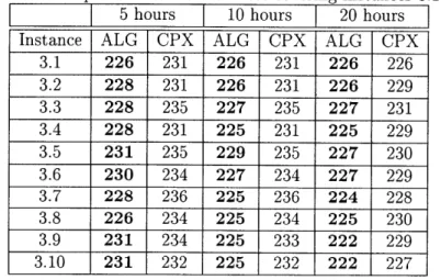
4.1-4.10 1000 2500 U[400,500] 3 5.1-5.10 1000 2500 U[400,500] 5 6.1-6.10 1000 2500 U[400,500] U[3, 7]The results from Table 2.2 to Table 2.7 compare the objective obtained from our binary optimization algorithm versus CPLEX 11.2 after 5-hour, 10-hour and 20-hour computational time. ALG denotes our binary optimization algorithm, and it is run by using the running sequence I; CPX denotes CPLEX 11.2, and it is run with its default settings. In the remainder of the thesis, we emphasize the better results in bold font in the comparison Tables.
Table 2.2: Computational results on set covering instances 1.1-1.10
5 hours 10 hours 20 hours Instance ALG CPX ALG CPX ALG CPX
1.1 346 344 344 344 344 343 1.2 346 343 344 343 344 342 1.3 346 345 344 345 344 344 1.4 343 345 343 345 343 344 1.5 344 346 343 343 343 342 1.6 344 345 344 345 344 343 1.7 343 343 343 343 343 342 1.8 344 345 342 345 342 343 1.9 343 345 343 345 343 344 1.10 344 346 342 346 342 344
For instances 1.1-1.10 in Table 2.2, after 5 hours, there are 60% instances that our algorithm outperforms CPLEX, while 30% instances CPLEX outperforms. After 10 hours, there are 60% instances that our algorithm outperforms CPLEX, while 10% instances CPLEX outperforms. After 20 hours, there are 40% instances that our algorithm outperforms CPLEX and 50% instances CPLEX outperforms.
Table 2.3: Computational results on set covering instances 2.1-2.10
5 hours 10 hours 20 hours
Instance ALG CPX ALG CPX ALG CPX 2.1 233 242 231 241 229 236 2.2 231 243 229 243 229 236 2.3 233 238 233 238 233 235 2.4 230 244 230 244 230 240 2.5 230 240 230 240 230 233 2.6 231 240 229 240 226 237 2.7 228 240 228 240 228 236 2.8 232 239 228 239 228 236 2.9 231 240 229 240 229 235 2.10 232 239 231 239 231 236
For instances 2.1-2.10 in Table 2.3, our algorithm outperforms CPLEX all the time.
Table 2.4: Computational results on set covering instances 3.1-3.10
5 hours
10 hours
20 hours
Instance ALG CPX ALG CPX ALG CPX
3.1 226 231 226 231 226 226 3.2 228 231 226 231 226 229 3.3 228 235 227 235 227 231 3.4 228 231 225 231 225 229 3.5 231 235 229 235 227 230 3.6 230 234 227 234 227 229 3.7 228 236 225 236 224 228 3.8 226 234 225 234 225 230 3.9 231 234 225 233 222 229 3.10 231 232 225 232 222 227
For instances 3.1-3.10 in Table 2.4, our algorithm outperforms CPLEX all the time.
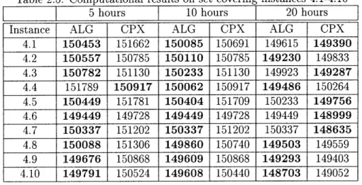
For instances 4.1-4.10 in Table 2.5, after 5 hours, there are 90% instances that our algorithm outperforms CPLEX, while 10% instances CPLEX outperforms. After 10 hours, our algorithm outperforms CPLEX for all instances. After 20 hours, there are 50% instances that our algorithm outperforms CPLEX and 50% instances CPLEX outperforms.
Table 2.5: Computational results on set covering instances 4.1-4.10
1_ 5 hours 10 hours 20 hours
Instance ALG CPX ALG CPX ALG CPX
4.1 150453 151662 150085 150691 149615 149390 4.2 150557 150785 150110 150785 149230 149833 4.3 150782 151130 150233 151130 149923 149287 4.4 151789 150917 150062 150917 149486 150264 4.5 150449 151781 150404 151709 150233 149756 4.6 149449 149728 149449 149728 149449 148999 4.7 150337 151202 150337 151202 150337 148635 4.8 150088 151306 149860 150740 149503 149559 4.9 149676 150868 149609 150868 149293 149403 4.10 149791 150524 149608 150440 148703 149052
Table 2.6: Computational results on set covering instances 5.1-5.10
1
5 hours
10 hours
20 hours
Instance ALG CPX ALG CPX ALG CPX
5.1 100264 107920 99663 107920 99663 103111 5.2 102454 107776 100943 107776 100131 102393 5.3 100266 107190 99837 105185 99837 100904 5.4 100393 106231 100393 106231 100393 101017 5.5 100341 107072 100180 107072 99911 102651 5.6 101272 106268 100585 106268 98989 101442 5.7 100718 107542 99978 107542 99978 102396 5.8 101070 108647 100530 108647 99651 103266 5.9 100592 106986 100288 106986 99970 103100 5.10 100084 108170 100084 108170 100084 102330
For instances 5.1-5.10 in Table 2.6, our algorithm outperforms CPLEX all the time.
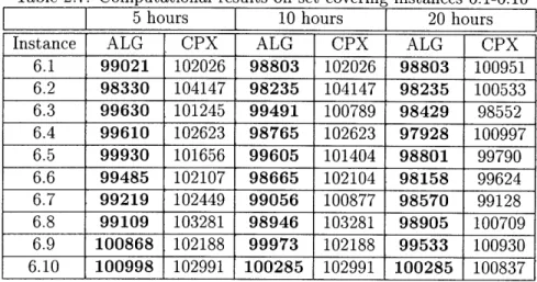
Table 2.7: Computational results on set covering instances 6.1-6.10
5 hours
10 hours
f
20 hours
3
Instance ALG CPX ALG CPX ALG CPX
6.1 99021 102026 98803 102026 98803 100951 6.2 98330 104147 98235 104147 98235 100533 6.3 99630 101245 99491 100789 98429 98552 6.4 99610 102623 98765 102623 97928 100997 6.5 99930 101656 99605 101404 98801 99790 6.6 99485 102107 98665 102104 98158 99624 6.7 99219 102449 99056 100877 98570 99128 6.8 99109 103281 98946 103281 98905 100709 6.9 100868 102188 99973 102188 99533 100930 6.10 100998 102991 100285 102991 100285 100837
For instances 6.1-6.10 in Table 2.7, our algorithm outperforms CPLEX all the time.
To conclude, for the set covering problems with 5 ones or 3 to 7 ones in each column of the constraint matrix A, our binary optimization algorithm strictly out-performs CPLEX at all time points when both methods are run with the same amount of memory (6GB). While for set covering problems with 3 ones in each column of the constraint matrix A, our algorithm is competitive with CPLEX. Therefore, our con-clusion is that our algorithm outperforms CPLEX for denser binary optimization problems.
The selection of
Q
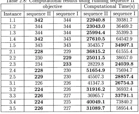
and MEM provides lots of flexibility for running the algorithm, and sequence I is not the best for every instance. We test another running sequence on instances 1.1-1.5, 2.1-2.5, 3.1-3.5, and refer to it as running sequence II.1. Q =6,MEM = 1GB 2. Q 10,MEM=6GB
The results in Table 2.8 show the advantage of using running sequence II. For 9 out of 15 instances, running sequence II converges faster and finds a better solution
(smaller objective) for minimization problems. Meanwhile, both sequences gave the same quality solution for 4 out of 15 instances.
Table 2.8: Computational results using running sequence II objective Computational Time(s) Instance sequence II sequence I sequence II sequence I
1.1 342 344 22940.8 39381.7 1.2 344 344 23043.0 36469.2 1.3 344 344 25994.4 35399.3 1.4 342 343 27610.5 64542.9 1.5 343 343 35435.7 34907.1 2.1 228 229 36815.2 61555.4 2.2 230 229 25011.5 38057.0 2.3 234 233 28229.8 24039.8 2.4 228 230 51654.9 75694.7 2.5 229 230 45507.3 28857.4 3.1 226 226 41347.3 26754.3 3.2 224 226 31916.2 36932.4 3.3 226 227 36965.7 33791.1 3.4 224 225 40049.1 73840.2 3.5 226 227 31089.7 58954.4
We also test our algorithm on random set packing instances with the following tunable parameters.
" m: the number of constraints " n: the number of binary variables
" c: the cost vector
" w: the number of non-zeros in each column of matrix A " U[l, u): random integer with its value between 1 and u
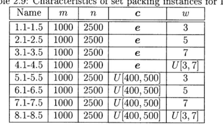
We generate 5 examples for each specific parameter settings listed in Table 2.9. For example, Instance 1.2 refers to the second example of type one instance. We test our implementation of the algorithm on those instances and compare the results with the output from CPLEX 11.2. All the tests are run on the Operations Research
Center computational machine. Instances 1.1-1.10, 2.1-2.10, 3.1-3.10, 4.1-4.10 are run on a machine with a Intel(R) Xeon(TM) CPU (3.00GHz, 2MB Cache), 8GB of RAM, and Ubuntu Linux operation system. Instances 5.1-5.10, 6.1-6.10, 7.1-7.10, 8.1-8.10 are run on a machine with Intel(R) Xeon(R) CPU E5440 (2.83GHz, 6MB Cache), 8GB of RAM, and Ubuntu Linux operation system.
Table 2.9: Characteristics of set packing instances for IP
Name
m
n
c
w
1.1-1.5 1000 2500 e 3 2.1-2.5 1000 2500 e 5 3.1-3.5 1000 2500 e 74.1-4.5
1000 2500
e
U[3, 7]
5.1-5.5 1000 2500 U[400, 500] 3 6.1-6.5 1000 2500 U[400,500] 5 7.1-7.5 1000 2500 U[400,500] 7 8.1-8.5 1000 2500 U[400, 500] U[3, 7]For those examples, we consider the CPLEX parameter MIP emphasis, which controls the trade-offs between speed, feasibility, optimality, and moving bounds in solving MIP. With the default setting of BALANCED [0], CPLEX works toward a rapid proof of an optimal solution, but balances that with effort toward finding high quality feasible solutions early in the optimization. When this parameter is set to FEASIBILITY [1], CPLEX frequently will generate more feasible solutions as it optimizes the problem, at some sacrifice in the speed to the proof of optimality. When the parameter is set to HIDDENFEAS [4], the MIP optimizer works hard to find high quality feasible solutions that are otherwise very difficult to find, so consider this setting when the FEASIBILITY setting has difficulty finding solutions of acceptable quality.
Since our algorithm also emphasizes on finding high quality feasible solution in-stead of proving optimality, we compare CPLEX's performance when the parameter
MIP emphasis is set as 0, 1, and 4, in order to find out which setting will deliver the
best solution. Based on the results in Table 2.10, we see that the results are consis-tently better than the default setting when MIP emphasis is set to be 4. Thus, in the following test, we run parallel experiments on CPLEX by setting the parameter MIP
emphasis as 0 and 4, respectively, in order to make a better
algorithm and CPLEX.
comparison between our
Table 2.10: CPLEX performance with different MIP emphasis settings
5 hours 10 hours 20 hours
Instance 0 1 4 0 1 4 0 1 4 1.1 319 320 319 319 321 321 322 323 322 2.1 155 159 161 155 160 162 155 162 162 4.1 255 252 258 255 253 258 258 256 259 5.1 147663 144054 148706 147663 144234 148894 148617 146525 149500 6.1 71799 73722 74865 71799 73722 75488 75594 75407 76806 8.1 113760 110979 115852 113760 111668 115852 114948 114157 115909
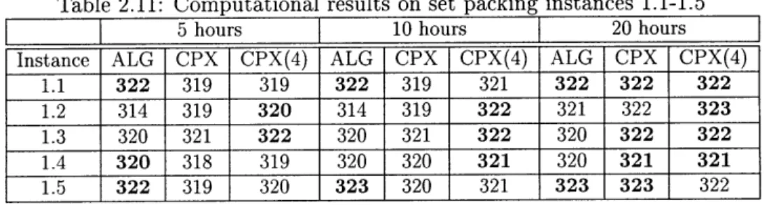
In the following test results from Table 2.11 to Table 2.18, ALG denotes our binary optimization algorithm, and it is run by using running sequence I; CPX denotes CPLEX 11.2, and it is run with default settings; CPX(4) denotes CPLEX 11.2 run with MIP emphasis 4. We run CPX(4) on selective instances, thus the star mark in the tables denotes the result is not available because no experiment is performed. We compare the results from our algorithm with the best practice from CPLEX if the results from CPX(4) are available.
Table 2.11: Computational results on set packing instances 1.1-1.5
T_ _ 5 hours 10 hours 20 hours
Instance ALG CPX CPX(4) ALG CPX CPX(4) ALG CPX CPX(4)
1.1 322 319 319 322 319 321 322 322 322
1.2 314 319 320 314 319 322 321 322 323
1.3 320 321 322 320 321 322 320 322 322
1.4 320 318 319 320 320 321 320 321 321
1.5 322 319 320 323 320 321 323 323 322
For instances 1.1-1.5 in Table 2.11, after 5 hours, there are 60% instances that our algorithm outperforms CPLEX, while 40% instances CPLEX outperforms. After 10 hours, there are 40% instances that our algorithm outperforms CPLEX, while 60% instances CPLEX outperforms. After 20 hours, there are 60% instances that CPLEX outperforms our algorithm and 40% ties.
For instances 2.1-2.5 in Table 2.12, our algorithm outperforms CPLEX all the time.
Table 2.12: Computational results on set packing instances 2.1-2.5
_ _ 5 hours 10 hours 20 hours
Instance ALG CPX CPX(4) ALG CPX CPX(4) ALG CPX CPX(4)
2.1 166 155 161 167 155 162 167 155 162
2.2 165 159 159 168 159 160 168 161 162
2.3 165 160 159 166 160 159 166 160 161
2.4 167 157 159 167 157 160 167 157 163
2.5 164 156 158 166 156 159 166 162 163
Table 2.13: Computational results on set packing instances 3.1-3.5
5 hours
10
hours
20 hours
Instance ALG CPX CPX(4) ALG CPX CPX(4) ALG CPX CPX(4)
3.1 104 95 95 105 95 97 105 98 100
3.2 103 95 95 106 95 95 106 95 98
3.3 105 95 95 105 95 97 105 95 100
3.4 105 97 96 105 97 96 105 97 99
3.5 105 97- 96 105 97 96 105 97 97
For instances 3.1-3.5 in Table 2.13, our algorithm outperforms CPLEX all the time.
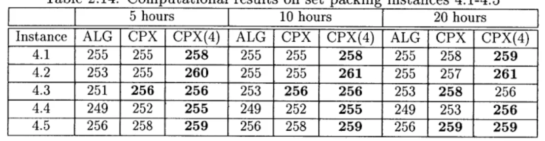
Table 2.14: Computational results on set packing instances 4.1-4.5
1_
5
hours
10 hours
20 hours
Instance ALG CPX CPX(4) ALG CPX CPX(4) ALG CPX CPX(4)
4.1 255 255 258 255 255 258 255 258 259
4.2 253 255 260 255 255 261 255 257 261
4.3 251 256 256 253 256 256 253 258 256
4.4 249 252 255 249 252 255 249 253 256
4.5 256 258 259 256 258 259 256 259 259
For instances 4.1-4.5 in Table 2.14, CPLEX outperforms our algorithm all the time.
For instances 5.1-5.5 in Table 2.15, CPLEX outperforms for all the instances. For instances 6.1-6.5 in Table 2.16, our algorithm outperforms CPLEX all the time.
For instances 7.1-7.5 in Table 2.17, our algorithm outperforms CPLEX all the time.
For instances 8.1-8.5 in Table 2.18, after 5 hours, CPLEX outperforms our algo-rithm all the time. After 10 hours and 20 hours, there are 80% instances that CPLEX
Table 2.15: Computational results on set packing instances 5.1-5.5
5 hours 10 hours 20 hours
Instance ALG CPX CPX(4) ALG CPX CPX(4) ALG CPX CPX(4)
5.1 146896 147663 148706 147800 147663 148894 148905 148617 149500 5.2 147796 147914 149511 147796 147914 149726 147796 149116 149726
5.3 147951 147479 148125 147951 147479 148733 147951 148583 148788
5.4 147421 147023 148568 147421 147023 148889 147421 148399 148889
5.5 148545 148208 149104 148545 148869 149325 148545 149261 149823
Table 2.16: Computational results on set packing instances 6.1-6.5
5 hours 10 hours 20 hours
Instance ALG CPX CPX(4) ALG CPX CPX(4) ALG CPX CPX(4)
6.1 75937 71799 74865 76590 71799 75488 77531 75594 76806 6.2 76928 72762 73080 77566 72762 73149 77566 74790 74752 6.3 76841 73447 74747 77681 73447 74747 77726 76086 75696
6.4 77475 72492 74392 77681 73231 74562 77681 75810 76299 6.5 76606 73361 73679 76985 73361 73750 77674 75376 74995
Table 2.17: Computational results on set packing instances 7.1-7.5
5 hours 1 10 hours 20 hours
Instance ALG CPX CPX(4) ALG CPX CPX(4) ALG CPX CPX(4)
7.1 48200 43708 45204 48200 43708 45577 48200 46052 46187 7.2 48559 43548 44001 48895 44579 45809 48895 45486 47083 7.3 48019 43433 44602 48019 44658 45177 48019 46287 45606
7.4 48297 43667 44517 48297 43667 45272 48297 45721 47383 7.5 48721 44046 45280 48721 44046 46767 48721 44641 47545
Table 2.18: Computational results on set packing instances 8.1-8.5
5 hours 10 hours 20 hours
Instance ALG CPX CPX(4) ALG CPX CPX(4) ALG CPX CPX(4)
8.1 114934 113760 115852 114934 113760 115852 114934 114948 115909
8.2 118242 117505 118261 118587 117505 118344 118587 118477 118447
8.3 116733 116896 118334 117115 116896 118334 117115 117686 118334
8.4 117227 116139 117317 117227 116421 117317 117227 117616 117317
outperforms our algorithm and 20% instances our algorithm outperforms.
To conclude, for set packing problems with 5 ones in each column of the constraint matrix A, our binary optimization algorithm strictly outperforms CPLEX at all time points when both methods are run with the same amount of memory (6GB). While for set packing problems with 3 ones or 3 to 7 ones in each column of the constraint matrix A, our algorithm is competitive with CPLEX. To support the conclusion that our algorithm outperforms CPLEX for denser binary optimization problems, we introduce another type of denser instances 4.1-4.5, 8.1-8.5, which have 7 ones in each column of the matrix A. The results are consistent with our assessment, that is, our algorithm outperforms CPLEX when the problem is dense. The new CPLEX setting
mip emphasis does not change the comparison results for most of the examples.
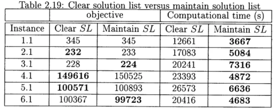
We also try to do some modifications to the algorithm. Our first attempt is to skip Step 7 SL <-
0,
that is, we do not clear the solution list after we find a better solution. The computational results on set covering instances 1.1-6.1 are shown in Table 2.19. The algorithm converges within one run with parameters:Q
= 10, MEM = 1GB. Here, we do not use a running sequence.Table 2.19: Clear solution list versus maintain solution list
I objective Computational time(s) Instance Clear SL Maintain SL Clear SL Maintain SL
1.1 345 345 12661 3667 2.1 232 233 17083 5084 3.1 228 224 20241 7316 4.1 149616 150525 23393 4872 5.1 100571 100893 26573 6636 6.1 100367 99723 20416 4683
The results in Table 2.19 show that when we maintain the solution list, the al-gorithm converges much faster, due to the fact that clearing solution list requires significant computational time. On the other hand, the solution quality is compara-ble to the original version.
Another idea is to search all the adjacent solutions of a solution x instead of leaving the neighborhood when a better feasible solution is found. If there is at
least one better feasible solution in the neighborhood of x, we continue to search the neighborhood and keep the best feasible solution. In the next iteration, we start searching the neighborhood of the updated best feasible solution. Otherwise, we extract a new solution x from the solution list.
The outline of the new algorithm is as follows.
1. x = zo; SL = x
2. while (SL f 0)
3. get a new solution x from SL
4. Y +- z
5. for each (y adjacent to x)
6. if (ATy ; b) & (cTy < cTy)
Y +- y 8. else if (y is interesting) TB[h(trace(y)} +- cry SL +- SL U y 11. if (Y f z) 12. SL- 0 13. SL -SL U Y 14. go to step 3 15. else 16. go to step 3
The computational results on set covering instances 1.1-6.1, 1,2-6.2 are shown in Table 2.20 compared to the results from the original algorithm. Both algorithms are run using the parameters
Q
= 10, MEM = 1GB instead of using a running sequence.Table 2.20: Comparison of the modified algorithm with the original algorithm
_ objective Computational time(s)
Instance ALG New ALG ALG New ALG
1.1 345 345 12661 13267 1.2 347 347 13091 12736 2.1 232 232 17083 17083 2.2 233 233 19449 19192 3.1 228 228 20241 21057 3.2 229 229 19441 19086 4.1 149616 150630 23393 26269 4.2 150994 149995 21211 30128 5.1 100571 99904 26573 25254 5.2 100362 101448 40129 24870 6.1 100367 100058 20416 34353 6.2 100694 100063 28395 24019
We have the following findings based on the results in Table 2.20, which show that the modified algorithm has competitive performance with the original algorithm.
1. The modified algorithm finds a better solution on some instances, for example, Instance 4.2, 5.1, 6.1, 6.2, while it converges to an inferior solution on Instance 4.1 and 5.2.
2. The modified algorithm converges faster on some instances, for example, In-stance 1.2, 2.2, 3.2, 5.1, 5.2, 6.2, while it converges slower on InIn-stance 1.1, 3.1, 4.1, 4.2 and 6.1.
Chapter 3
An Adaptive Local Search Algorithm
for Mixed Integer Optimization
3.1
Problem Definition
We consider the following problem to test our mixed integer optimization algorithm.
max cTx + dTy (3.1)
s.t. Ax +By ; b
x E
{O, 1}"1, y > 0where A E {O, 1}"xnl, B E {O, 1}Ixn2,b E
Q
,c EQ, d E Q .This problem is referred to as the set packing mixed integer problems (MIP).
3.2
Algorithm
We test the binary optimization algorithm proposed by Bertsimas and Goyal
18].
The algorithm takes as inputs the matrices A, B, the vectors b, c, d, parametersQ
and MEM, and an initial solution (zxo, zy0). The algorithm generates a series of feasible solutions with monotonically increasing objective values during the searchprocess. The parameter
Q
controls the search depth of the searching neighborhood, which poses a trade-off between solution quality and computational complexity. The parameter MEM controls the size of the solution list, which affects the degree of collision of interesting solutions with similar characteristics in constraint violation and looseness.We divide the solution into two parts: x and y(x), which stand for the solution to the binary variables and the solution to the continuous variables, respectively. As introduced in Section 2.2, we consider the following definition.
" V(x) = max(Ax - b, 0) E Z': the amount of constraint violation produced by x.
" U(x) = max(b - Ax, 0) E Z': the amount of constraint looseness produced by x.
* W(x) = min(U(x), e) E {0, 1}m
" trace(x) = [V(x); W(x) - W(zx)] E Zm x {0, 1}m, Let zx to be the solution to the binary variables of the current best solution at a certain iteration of the algorithm.
* Two solutions x1 and x2 are said to be adjacent if eTlxi - x2
1
1." A feasible solution (zi, y(zi)) is said to be better than another feasible solution (z2, y(z 2)) if (cTzi + d'y(zi)) - (cT z2 + d'y(z2)) > 0.1.
The solution to the continuous variables is computed given the solution to the binary variables by solving
arg max{d
Ty
By b-Ax,y>0}, Ax<b
0 Ax> b
" A solution x is said to be interesting if the following three criteria hold: (Al)
|IV(x)||oo <
1: no constraint is violated by more than one unit. (A2) The number of violated constraints incurred by x is at mostQ.
(A3) (czTx + d'y(x)) - (cTX' + dTy(x')) > 0.1, Vx'already examined such
that h(trace(x)) = h(trace(x')). h(.) is a linear function that maps a vector into an integer. The mapping is multiple-to-one, that is, different vectors may be mapped to the same integer. The specifications of h(.) are the same as the binary optimization algorithm in Section 2.3.
" A solution list SL
The solution list stores the solutions to the binary variables, which satisfies the criteria of interesting solutions. They are ordered according to their assigned priority values. The definition of priority value is the same as the definition in Section 2.3. The solution with the highest priority is extracted first.
" A trace box TB
The trace box entry TB[il stores the best objective among all of the interesting solutions (x, y(x)) satisfying h(trace(x)) = i.
In our implementation, we change some specifications of the algorithm compared to the original one in paper [8].
We only consider violation and looseness incurred by the solution to the binary variables (equivalent to assuming all the continuous variables are zero). Thus, the definitions of V(x), W(x), trace(x) are similar to the binary optimization algorithm. We use the criterion that the number of violated constraints instead of the total amount of violation cannot exceed
Q.
We update the best feasible solution and the interesting solution only when there is an numerical improvement of objective that is greater than or equal to 0.1. Here, we do not consider an improvement less than 0.1 appealing.More specifically, we give an outline of the algorithm as follows.
Input: matrices A, B; vectors b, c, d; feasible solution (zz0, zYO); scalar parameters Q,MEM
1. (zr, zv) = (z,0, z.0); SL = z, [MEM is specified to determine the size of the SL|
2. while (SL z 0)
3. get a new solution i,, from SL
4. for each (x adjacent to i) 5. if (Ax < b)
6. compute y(x) by solving argmax{dTy
I
By< b - Ax, y > 0}
7. if (cTx + d Ty(X)) - (CTZ + dTy(zY)) > 0.1 8. (zz, zy) +-- (X, y(x))
9. 12 +- x
10. go to step 4
11. else if (x is interesting [Q is specified for condition A2]) 12. TB[h(trace(x))] +- cTx + d Ty(x)
13. SL +- SL U x
14. else if (x is interesting [Q is specified for condition A2})
15. TB[h(trace(x))) +- cx + dTy(x), here y(x) is a zero vector SL +- SL U x
17. return zx
We divide the problem into a pure binary optimization subproblem and a linear optimization subproblem. We first solve the pure binary optimization subproblem max{cTx| Ax < b, x E {0, 1}1} by using the similar idea as the binary optimization algorithm in Section 2.2. The continuous solution is computed given the solution to
the binary variables by solving max{dTy
I
By < b - Ax, y > 0}. The algorithm starts with an initial feasible solution. In each iteration, the algorithm selects a candidate solution ix from the solution list SL and examines all of its adjacentsolutions. If any adjacent solution is interesting (refer to the definition of interesting solutions in Section 3.2), we store it in the solution list and update the appropriate trace boxes. If we find a better feasible solution zx, we jump to solution zz. The previous procedure resumes by examining the adjacent solutions of zx. Based on the results in Table 2.19, we maintain the solution list when a better feasible solution is found since it yields comparable results, but converges much faster compared to clearing the solution list.
3.3
Implementation Details
In order to utilize the memory efficiently, We use the following data structure to store the problem and the solution.
" We store the matrices, A, B and the vectors V(x), U(x), W(x) as sparse ma-trices and sparse vectors respectively, i.e., only store the indices and values of nonzero entries.
" We store only the binary solution x in the solution list not the corresponding continuous solution y, because we only need the partial solution x to construct its neighborhood.
" We store the partial solution vector x in binary representation, which decreases the storage commitment for a solution x from n to (sie (int) + 1) integers. " We use the same specifications of hash functions and the same method to extract
a new solution from the solution list as described in Section 2.3.
When we search the neighborhood of a solution ix extracted from the solution list, if its adjacent solution x is feasible, we call CPLEX to solve the linear optimization subproblem max{dTy