3D Snap Rounding

HAL Id: hal-02393625

https://hal.inria.fr/hal-02393625

Submitted on 4 Dec 2019

HAL is a multi-disciplinary open access

archive for the deposit and dissemination of

sci-entific research documents, whether they are

pub-lished or not. The documents may come from

teaching and research institutions in France or

abroad, or from public or private research centers.

L’archive ouverte pluridisciplinaire HAL, est

destinée au dépôt et à la diffusion de documents

scientifiques de niveau recherche, publiés ou non,

émanant des établissements d’enseignement et de

recherche français ou étrangers, des laboratoires

publics ou privés.

3D Snap Rounding

Leo Valque

To cite this version:

Author: Valque L´

eo

Master d’Informatique Fondamentale

Ecole Normale Sup´

erieur de Lyon

Master II Intership Report

3D Snap Rounding

Supervisor: Sylvain Lazard

[email protected]

INRIA

LORIA

Gamble Team

Contents

1 Introduction 2

1.1 Need for 3D Snap Rounding . . . 2

1.2 Formal Statement . . . 2

1.3 2D Snap Rounding . . . 3

1.4 3D Snap Rounding . . . 4

2 3D Snap Rounding Algorithm 4 2.1 Introduction . . . 4

2.2 Step 1: Collapse the faces that are close to one another . . . 4

2.3 Step 2: Partition the space into xy-parallel slabs . . . 5

2.4 Step 3a: 2D snap in thin slab to prepare triangulation . . . 6

2.5 Step 3b: Triangulation of the faces in thick slabs . . . 7

2.6 Correctness and complexity . . . 8

3 Algorithm implementation 9 3.1 2D Snap Rounding Implementation . . . 9

3.2 Step 1 Implementation . . . 10

3.2.1 Difficulties . . . 10

3.2.2 Step 1 in a Thick Slab . . . 11

3.2.3 Segment Tree . . . 13

3.3 Step 2 implementation . . . 13

3.3.1 Arrangement on the floor . . . 13

3.3.2 Lift the arrangement . . . 13

3.4 Efficient cut of Faces . . . 14

4 Result of the implementation 15 5 Improvement of the algorithm and the implementation 17 5.1 Lazy algorithm . . . 17

5.2 Test of proper intersection . . . 18

5.3 Lifting only in thick slabs . . . 19

5.4 Avoid exact calculations . . . 19

6 Summary of the work performed 19

7 Conclusions and Perspectives 20

Appendix

22

A Polygon difference 22

B Halfedge Data structure 22

1

Introduction

The problem of snap rounding consists in rounding the vertex coordinates with a certain guarantee on topology and geometry. We will first explain why snap rounding is necessary. Then, we will describe a solution to this problem in 2D and why it cannot be generalized in 3D. Then, we will describe the only existing solution in 3D for fixed grid. The goal of the internship was to implement, evaluate and improve this solution. We will present our implementation of this algorithm and then how to improve the algorithm and the implementation in the future.

1.1

Need for 3D Snap Rounding

Rounding 3D polygonal structures is a fundamental problem in computational geometry. Indeed, many implementations dealing with 3D polygonal objects, in academia and industry, require as input whose vertices have coordinates given with fixed-precision representations (usually with 32 or 64 bits). On the other hand, many algorithms and implementations dealing with 3D polygonal objects in computational geometry output polygons whose vertices have coordinates that have arbitrary-precision representations.

For instance, when computing boolean operations on polyhedra, some new vertices are defined as the intersection of three faces and their exact coordinates are rational numbers whose numerators and denominators are defined with roughly three times the number of bits used for representing each input coordinate (Fig. 1). This discrepancy between the precision of the input and output of many geometric algorithms is an issue, especially in industry, because it often prevents the output of one algorithm from being directly used as the input to a subsequent algorithm.

Figure 1: Example of intersection of four icosahedra. Image from Zhou et al. 2016 [17].

In practice, coordinates are often rounded without guarding against changes in topology and there is no guarantee that the rounded faces do not properly intersect one another. This naive rounding can make improper data that cannot be use after. In 3D, There are 2 possible types of intersection: a vertex that traverses a face or an edge that traverses an other edge.

For example, on a dataset of 10K meshes from thingiverse called thini10K, about half of the meshes have self-intersections. During mesh repair on this dataset , the naive snap rounding fails on 2.2% of cases [17].

1.2

Formal Statement

Given a set of disjoint-interior faces in 3D, the problem is to subdivide the faces and round the vertices so that no two disjoint faces map to faces that properly intersect during motion. For clarity, all schemes consider that vertices are rounded on the integer grid.

In such schemes, disjoint faces may collapse but this is inevitable if the rounding precision is fixed and if we bound the Hausdorff distance between one of each of them and their rounded images (Fig. 2).

Figure 2: Example of necessary collapsing if the Hausdorff distance is bounded.

Furthermore, it is NP-hard even in 2D to determine whether it is possible to round simple polygons with fixed precision and bounded Hausdorff distance, and without changing the topological structure [14]. So subdivisions may be needed.

The partical problem is to round the coordinates with a fine precision such as float or double.

1.3

2D Snap Rounding

The same problem in 2D for segments, referred to as snap rounding, has been widely studied and admits practical and efficient solutions [2, 5–8, 10–12, 15].

We describe one solution for 2D snap rounding. Let L the list of the input segments (Fig. 3), for each intersection or boundaries of segments, we create a ”hot ” pixel (Fig. 4) (a pixel is a unit square centered on the integer grid). If a segment goes through a hot pixel, we split it in 2 (Fig. 5). Then we can move old and new vertices to the center of their pixels without intersection (Fig. 6).

Figure 3: Input of segments for 2D snap. Figure 4: We label hot all pixels that contain an endpoint of a segment or an intersection.

Figure 5: We split all edges that intersect go through a hot pixel.

1.4

3D Snap Rounding

In this context, there exist only 2 algorithms for rounding the coordinates of 3D polygons with the constraint that their rounded images do not properly intersect and that every input polygon and its rounded image remain close to each other (in Hausdorff distance). The first one was presented by Fortune [4]. But this algorithm is very complicated and only works on a grid whose size depends on the number of vertices by 1/n. The second algorithm works with a fixed grid size independant of the input and will be described in the next section [3].

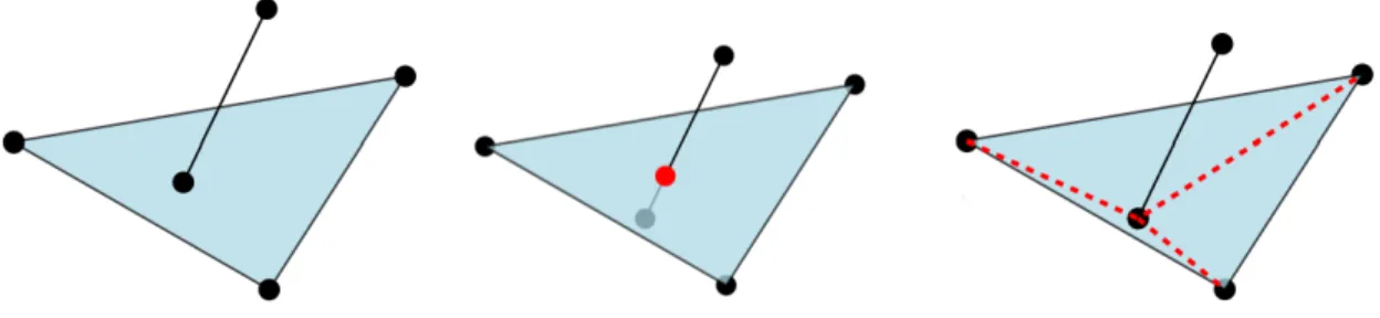
To understand why 3D snap rounding is difficult, note first that it is reasonable to round every vertex to the center of the voxel containing it (a voxel is a unit cube centered on the integer grid). But, by doing so, a vertex may traverse a face and to avoid that, it might be necessary to add beforehand a vertex on the face, which requires triangulating it (Fig. 7). Newly formed edges may cross other edges when snapping. To avoid this, new vertices maybe added to these edges, in turn requiring further triangulating of the faces. It is not known whether, there exist such schemes that always terminate. During mesh repair on Thingi10K, after 20 recursions of this scheme, 0.05% of the meshes have always self-intersections [17]. Further difficulties of snap rounding faces in 3D is described by Fortune [4].

Figure 7: Subdividing faces to avoid vertex-face traversing requires creating new edges that can induce new intersections.

2

3D Snap Rounding Algorithm

2.1

Introduction

We describe the algorithm presented by Devillers, Lazard and Lenhart for solving the snap rounding problem [3]. Recall that this is the first and only algorithm that solves the problem with a grid size that is independant combinatorial size of the input. This algorithm is divided in 4 steps:

• Step 1: Collapse the faces that are close to one another • Step 2: Partition the space into yz-parallel slabs • Step 3: Triangulate the faces

• Step 4: Round all vertices to their voxels centers

We detail each of them below. In what follows , the xy-plane is named the floor and the xz-plane is named the backwall.

2.2

Step 1: Collapse the faces that are close to one another

For each face Fi, we project it on faces F1 to Fi−1in this order. The projection of Fi to Fj such that for

the faces connected, we create walls between parts of the original face and the projected parts (Fig. 8)-(Fig. 9). This step gives the property that for each face F , there are no faces at distance less than 1 along y except for the connecting walls that we created.

Figure 8: Projection of Step 1, the red part is the projected part, the orange parts are walls created to keep the projection of Fi connected.

Figure 9: Example of step 1 projection in 3D.

2.3

Step 2: Partition the space into xy-parallel slabs

We project all faces obtained by Step 1 on the floor, we obtain a 2D arrangement. An arrangement of segments is the partition of the plane formed by these segments. For each facet of this arrangement, we lift it on all faces above it (Fig. 10). So after this step, for all pair of faces, their projection on the floor are equal or interior disjoint.

Figure 10: Floor projection of the 3D faces and lift of the facets of the floor arrangement on the 3D faces. Then we partition the space into slabs (Fig. 11). There are 2 types of slabs. A Thin Slab is a closed region bounded by two side walls x = c ±1

2f orc ∈ Z. So a thin slab will be rounded onto his middle plane. A

Thick Slab is a closed region bounded by two consecutive thin slabs (it can have 0 width). We create a thin slab for each vertex of the 2D arrangement on the floor. A thin slab may contain several of such vertices. With this, there are no vertex in thick slabs.

Figure 11: Representation of thick and thin slabs. Figure 12: Cut faces by the walls between slabs. Then, we project the faces on the backwall and we create a thin slab for each vertex of the induced arrangement. Then we cut the faces by the slab boundaries (Fig. 12). With this, no two edges in a thick slab intersect each other on the backwall projection.

2.4

Step 3a: 2D snap in thin slab to prepare triangulation

In a thin slab, faces will be rounded on a single plane, so the problem become 2D and we can solve it with a 2D snap rounding (Fig. 13a). First, we project the edges on the middle plane and then we snap them in 2D

(Fig. 13b). Then we do a L1 projection of the created vertices by the 2D snap on their original edges (Fig. 13c). This step can create vertices in the side walls shared with the adjacent thick slabs.

(a) Faces in a thin slab. (b) Some vertices are created by the projection and 2D snap in the middle plane.

(c) We lift these vertices on their original edges.

Figure 13: Step 3a.

2.5

Step 3b: Triangulation of the faces in thick slabs

After treating all thin slabs, we can continue with thick slabs (Fig. 14). In a thick slab, faces are trapezes. To keep planar faces after rounding, we need to triangulate them. Thanks to Step 2, all faces have identical or interior disjoint floor projections. To ensure that triangulation edges do not intersect after snapping, we define them so that their floor projections are identical or interior disjoint. So we add edges that link the ”top-left” vertex of each trapeze with its ”bottom-right” vertex (Fig. 15) (viewed in projection on the floor).

Figure 14: Faces in a thick slab. Figure 15: We triangulate faces by top-left to bottom-right diagonals.

During Step 3a, we could have created new vertices on the walls of the slab, so we need to triangulate these points as well (Fig. 16). After these steps, vertices can be rounded without creating intersections (Fig. 17).

Figure 16: Trapeze triangulations with vertices

induced by adjacent thin slabs. Figure 17: We can round safely.

2.6

Correctness and complexity

The proof of correctness of this algorithm is complicated and described in the original paper [3]. To compute the complexity, we count the number of lines supporting edges instead of the number of edges.

• Step 1 : we can do Step 1 by considering the arrangement on the backwall and lift it back. If we have O(n) supporting lines in the input, we have O(n) lines on the backwall and each line can be lifted onto O(n) faces so we have after this step at most O(n2_{) lines in the scene.}

• Step 2 : we project lines on the floor and then lift them back. Lifting on the O(n2_{) connected walls}

created by Step 1 is not necessary [3]. We have at most O(n2) lines on the floor and each one can be lifted onto the n faces. So we have at most O(n3_{) lines in the scene after the lifting.}

we project these lines on the back to compute thin slabs. An arrangement of O(N ) lines has at most O(N2_{) intersection points so with N = n}3 _{we have at most O(n}6_{) intersection points so at most O(n}6₎

slabs.

we cut the O(n3) faces of the scene by these O(n6) slabs so we have at most O(n9) faces, O(n3) per slab.

• Step 3a : 2D snap rounding can create O(N3_{) vertices for an input of size O(N ) so we can have O(n}9₎

vertices per thin slab. O(n15) vertices in all slabs.

• Step 3b : in a thick slab, we create an edge for each face and for each vertex created by adjacent slabs. There are at most O(n3_{) edges inside the slab and at most O(n}9_{) vertices created by adjacent slabs. So}

we have at most O(n9) edges in the slab.

So with all steps, we have at the end a space complexity of O(n15_{). The time complexity is O(n}16,5_{) [3].}

With some assumptions, the complexity decreases to O(n5) in space and O(n6,5) in time [3]. But if edges are ”small” and vertices are ”well distributed”, intersection will be ”rare” and we can expect O(n) slabs in practice. In a ”distributed” setting too, cutting a scene by a plan hits O(√n) faces so we can expect O(n√n) in practice. One of the goals is to evaluate if these assumptions are correct.

3

Algorithm implementation

The goal of the internship was to implement, evaluate and improve this algorithm using the CGAL library [16]. CGAL provides us some usefull package :

• A representation of 3D scenes named halfedge data structure (see next paragraph).

• An implementation of 2D arrangement as input a set of 2D segments and output an halfedge data structure on the 2D plane.

• An implementation of 2D snap rounding.

To implement this algorithm, we use the halfedge data structure (Fig. 18) [13]. Each halfedge h goes from a source vertex s to a target vertex t (also called incident vertices). h has a pointer on his adjacent face f . Its opposite halfedge has for source t and target s and a different adjacent face. The next halfedge of h is the halfedge with source t and the same adjacent face f . The previous halfedge has target s and the same adjacent face too. The halfedge data structure implements some operations on structure like split a facet or an edge (Annexe B).

The big advantage of the halfedge data structure is that if we modify a face of the scene, all adjacent faces will automatically be modified. With it we can easily manage the creation of vertices. The disadvantage of the halfedge structure is it does not really manage the edges adjacent to more than 2 faces (we have to duplicate edges and vertices in this case).

We describe in the next section the implementation of Step 1 and Step 2. The implementations of Step 3 and Step 4 are really simple and we will not describe it.

Figure 18: Representation of the halfedge Data Structure. Image from CGAL Documentation [16].

3.1

2D Snap Rounding Implementation

When we used the 2D snap rounding of CGAL, this one was surprisingly slow. After some research, we discover that this package of CGAL was old and not optimized and so we reimplemented it.

We implemented the algorithm describes in Section 1 1.3 [7]. To find pixels that need to be ”hot, we compute the intersection points with the 2D Arrangement package of CGAL. Then, for each ”hot” pixels (x, y), we add the segments [(x + 0.5, y + 0.5), (x − 0.5, y − 0.5)] and [(x − 0.5, y + 0.5), (x + 0.5, y − 0.5)] to

Figure 19: Factor acceleration of our implemen-tation compared to CGAL implemenimplemen-tation. The input is n random segments of length O(√n).

Figure 20: Factor acceleration of our implemen-tation compared to CGAL implemenimplemen-tation. The input is n random segments of length O(1).

the arrangement, these segments form a cross in this pixel. For each segment of the input, if it goes through a hot pixel, it necessarily intersect this cross and this segment is cutted. Then we can round the points. The majority of operations are done by the arrangement package of CGAL and not by us.

We compared our implementation and the implementation of CGAL on random inputs of different size (Fig. 19). Inputs was segments of length O(√n), on average, we have O(n) intersections of segments. For all input, the 2 implementations give the same output. For running times, the 2 implementations seem to have not the same complexity. Our implementation take 6 less times for the largest tested input. Test with segments of length O(n) gives the same result, on average, we have O(n2_{) intersections of segments. Our}

implementation is 2 times slower for segments of length O(1), on average, we have O(1) intersections of segments (Fig. 20).

3.2

Step 1 Implementation

3.2.1 Difficulties

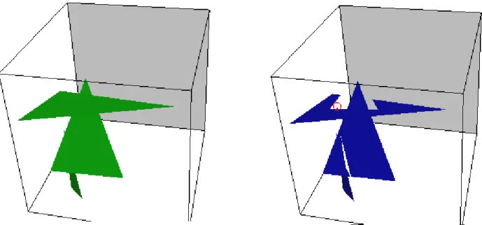
In Step 1, we need to project faces that are close to one another. When a face F is projected, possibly only a part of F is projected. So we need to continue with the projections of the rest of F onto the other faces. Problem, the difference of 2 convex polygons can be non-convex non-connected polygons with holes (Fig. 21). Managing side walls with these non-convex non-connected polygons with holes is a nightmare to implement. To avoid this problem, we have modified Step 1.

Figure 21: Example of projection of Step 1 (the connected walls are not drawn). We can see a hole in the middle triangle and a quite complicated form of the top triangle (there is a tooth inside the red circle).

3.2.2 Step 1 in a Thick Slab

We present a modification of the algorithm in Section 2. We split Step 1 into two parts. We do the first part at the beginning of the algorithm and the second just after the cutting by the walls (between Step 2 and Step 3).

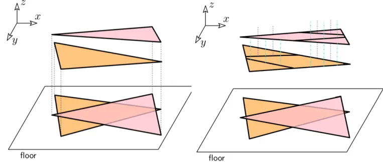
In the first part, for each pair of faces A and B, we calculate the intersection lines between planeA with

planeB± ~ and planeA± ~ with planeB and then we cut the faces A and B by these 2 lines (Fig. 22). So

after this cutting, if a part of a face A0 is at distance less than 1 along y of a face B0, then all A0 is at distance less than 1 of B0 (Fig. 23).

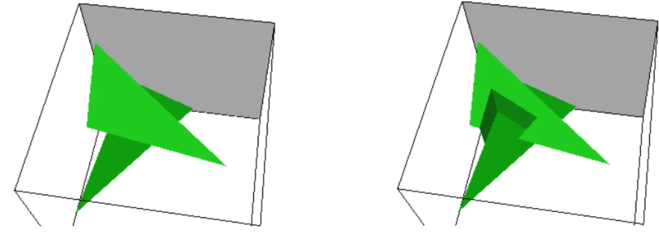
In the second part, so righ after Step 2, we perform the projection described in Step 1 in all thick slabs. In thick slabs, the faces are trapezoids without intersection between the edges in the back-wall projection. The difference of such trapezes can only be same kind of trapezes, so we avoid holes and non-convexity (Fig. 24). The projections and building of the walls are really simplified.

With this projection, we create new edges and faces such that the equal or disjoint floor projection property can be lost. To avoid this, during the first part of the modified Step 1, we add the projection of the face A on the planeB and the projection of the face B on the planeA. Does this is brutal and unefficient

and was only done to have a complete algorithm before the end of the internship. A proper modification is simply to repeat Step 2 in the thick slab. However, degeneracies are produced by projections and need to be managed (see (Annexe C)).

Figure 22: We calculate the intersections of planeA with planeB± ~ and of planeA± ~ with planeB. Then

we cut A and B by these 2 lines.

Figure 23: After Step 2, we project the faces in thick slab.

Figure 24: The only 2 possible cases of faces projection on the back wall inside a thick slab.

We have modified the algorithm so that we have to justify the correction of this change. Lemma 2 of Devillers, Lazard and Lenhart’s article states that during the projection of Step 1, Hausdorff’s distance before and after the rounding never exceeds 1 and the topology is preserved up to collaspe [3]. Lemma 3 of the same paper states that after Step 1, the distance along y between 2 points of different faces is at least 1. The modification of Step 1 described below respects the assumptions of these lemmas. So the proof of correctness inside thick slabs is unchanged. Inside thin slabs, these lemmas are not used and the proof is also unchanged.

3.2.3 Segment Tree

The projection of Step 1 must project all faces on all others, rigorously, it is a O(n2_{) but we project only over}

a distance less than 1. We optimize it with segment trees [1]. We can approximate faces by its bounding box and project them only if their bounding boxes are at distance of less than 1. With segment trees, recovering the intersections of n boxes has for complexity O(nlog(n) + k) where k is the number of intersections.

3.3

Step 2 implementation

3.3.1 Arrangement on the floor

After computing the floor arrangement, for each facet of this arrangement, we must find all 3D faces that are above. Arrangement package of CGAL takes segments as input and it does not give us this. To do this, we color all input segments with the indexes of its adjacent faces and store one oriented segment for each 3D face (Fig. 25). An edge can have many adjacent faces so can have as much colors.

Then for each 3D face, we make the following algorithm (Fig. 25). We color the adjacent 2D facet of the stored segment with the index of the 3D face. Then, for each boundary edge of this facet, if the segment of this edge does not have the color of this 3D face, we color the facet on the other side of this edge and we repeat this process for this facet. Repeating this process for each face implies that facets may have several colors.

Now, we have the 3D faces above 2D facets, we can lift them.

(a) (b) (c)

(d) (e) (f)

Figure 25: (a) We color segments by the indexes of the adjacent faces (here segments have only one adjacent triangle). (b) (c) For the blue triangle, we color the facet adjacent to the remember segment. (d) (e) (f) If an edge of the boundary doesn’t have the same color as the facet considered, we color the facet on the other side and repeat for this facet.

3.3.2 Lift the arrangement

To lift the facets, we simply project them onto all planes of the 3D faces above.

The floor facets can have complex shapes and we therefore prefer to completely rebuild the scene instead of trying to modify it. But we have to keep connectivity between faces so if 2 faces share a vertex, it must be lifted to a single vertex.

To do this, for each vertex of the 2D arrangement, we store all 3D vertices already lifted from this 2D vertex. Each time we lift a facet F on a plane A, for each 2D vertex of that facet, we check if we have already created a 3D vertex on that plane, if that is true we take that point, otherwise we create a new vertex.

3.4

Efficient cut of Faces

Cutting a scene by a plane has complexity O(n) where n is the number of edges. Unless the grid is rough, we have at least O(n) slabs (we create one slab per vertex). If we make a naive cut, we have a complexity of O(n ∗ s) = O(f ∗ l ∗ s) where s is the number of slabs, f the number of faces and l the mean size of a face. We will present an efficient way to cut a face by slabs (Fig. 26).

First, find the left vertex of the face and we target the wall to the right of this vertex. We were going to go through the edges clockwise. If an edge goes from left to right, if it crosses the target wall, we split the edge , stack the created vertex and target the next wall. If one edge goes from right to left, we target the previous wall. If it crosses the target wall, we split the edge, target the previous wall and link the created vertex with the top of the stack (Fig. 26).

With this small algorithm, cutting a face F by s slabs is O(log(s) + k + l) where k is the number of slabs that truly cutting F and l the size of the face. So we have a general complexity of O(f ∗ (log(s) + k + l)) = O(n + f ∗ (log(s) + k)) which is really smaller than the naive algorithm.

(a) (b) (c)

(d) (e) (f) (g)

(h) (i) (j) (k)

(l) (m) (n) (o)

Figure 26: (a) We want to cut a face by walls of slabs. (b) We start from the left vertex, and we target the wall on right of this vertex.(c) (d) (g) We were going to go through the edges clockwise.(e) (f) (h) If the edge goes from left to right, and if it crosses the target wall, we split the edge, stack the created vertex and target the next wall.(i) (m) If the edge goes from right to left, we target the previous wall.(j) (l) (n) If it crosses the target wall, we split the edge, target the previous wall and (k) (l) (o) we link the created vertex with the top of the stack.

4

Result of the implementation

We tested our implementation (without Step 1) on a polyhedron of a aircraft of around 70.000 faces with a rough grid size (Fig. 27). The output has a voxelated appearance that is not the desired behaviour. This algorithm makes no sense in the context of a rough grid.

Figure 27: Test of the algorithm on a plane. The output has a voxelated appearance.

The problem is that the algorithm becomes very slow and has a very large output when we take a very fine grid. The cause is the number of thin slabs. with a very fine grid, we can expect as many thin slabs as the number of vertices in the bottom arrangement (5.000.000 vertices in the backwall arrangement for the aircraft).

The running time is dominated by the 2D snap in the thin slabs and so adds thin slabs taking more time. With this, it is impossible to run the algorithm on very fine grid except for very small input.

To evalutate the complexity, we compute the size of the backwall arrangement on 250 elements of the Thingi10k Dataset [18]. On a log-log scale, we obtain a scatter plot that is concentrated around a line (Fig. 28). A linear interpolation gives us a size of the backwall arrangement of 141n1.13 _{where n is the number of}

vertices in the input. We can interpret these results as the backwall arrangement being linear or almost-linear but with a significant prefactor and a significant variance. Therefore, the assumption that the backwall arrangement is linear was correct such that the algorithm has the expected space complexity of O(n ∗ sqrt(n)) in practice. But with a significant prefactor, this complexity is actually too large to use in practice.

So the algorithm is unusable in this form, for very fine grids. But the trivial rounding works on the majority of vertices so we can design a lazy algorithm that makes trivial rounding where are possible and do the heavy algorithm where are needed.

Figure 28: Number of vertices of the Backwall Arrangement function of number of vertices of the input in log-log scale. The points are noisy but we interpolate a line with slipe of 1.13 and value on 0 of 2.15 so we have y = 10b_{∗ x}a_{= 141n}1.13

.

5

Improvement of the algorithm and the implementation

We have described the implemented version of the algorithm but improvements are needed to have a usable version. In this section, we present different ways to improve the algorithm in the future.

5.1

Lazy algorithm

The standard algorithm is slow and returns an output that is too large for fine grids. We know that the trivial rounding works most of the time [17]. The idea is therefore to run the heavy algorithm only where it is needed.

First, we have to detect problematic elements. For each vertex-face or edge-edge pair, we check if the 2 elements risk to intersect when continuousy snap rounding the vertices (Fig. 5.2). If they intersect, the concerned vertices, edges or faces are ”frozen”.

We isolate the frozen elements in work slabs (Fig. 29). For each problematic intersection, we create a work slab that starts from the largest x ∈ Z smaller than the x-coordinate of the vertices of the frozen elements and ends at the smallest x ∈ Z larger than the x-coordinate of the vertices of the frozen elements.

These slabs are bounded by walls and we cut the edges that traversing these walls. By cutting the edges, we create new vertices and faces need to be triangulated.

We have to check if the edges of the triangulation don’t create new problems. If the new edges create a new intersection, we go back before cutting by the walls of the work slabs. Now, we double the width of the work slabs and try again.

(a) (b)

(c) (d) (e)

(f) (g) (h)

Figure 29: (a) For a scene. (b) We find some problematic elements. (c) They are isolated in work slabs. (d) We cut through the slab walls and triangulate the faces. (e) (f) If there is a problem with the new edges, go back, double the width of work slabs and try again. (g) (h) If there are no problems, we make the heavy algorithm in work slabs and trivial rounding on the outside.

5.2

Test of proper intersection

For the vertex-face intersection, if the motions are linear to the voxel centers, computing the intersection amounts to compute a determinant of degree 6 amounts to solve a polynomial of degree 3 (defined by a 4x4 determinant). Then for these roots, it should be determined whether the corresponding plane-line intersection points lie in the moving face. To avoid these complicated computations, we propose the following scheme in which instead of moving each vertex in a straight line to its voxel center, we first round in x, then y then z. In what follows, orientation is the sign of the determinant of 4 points in homogeneous coordinates.

First, we round the x-coordinate. Thus, the projection on the yz-plane doesn’t change with the snap. To check if a vertex traverses a face, the orientation of the 4 points before and after the rounding is calculated. If the orientation has changed, it is possible that the vertex and the face intersect each other. Next, we check if the projection of the vertex in yz-plane is in the face, if that is the case then they intersect each other, otherwise they do not.

Then we do the same thing on y and z. If there is an intersection on at least one of the 3 coordinates, the 2 elements properly intersect.

We do something very similar for edge-edge intersection. First we move on x. As for the vertex-face intersection, we check if the orientation of the 4 points has changed. If the orientation has changed and the projection of edges in yz-plane intersects, they intersect each other in 3D. Then we round on y and z.

This checker was implemented during the internship. As accelerator, we used the Segment tree described in Section 3 3.2.3. With this accelerator, we check if 2 elements intersect each other only if they are closed.

5.3

Lifting only in thick slabs

We observed in our experiments that most of the time is spent in thin slabs. So, to improve the running time it may be useful to reduce the number of vertices and edges in the thin slabs. Lifting the faces from the floor is only necessary in thick slabs so the goal is to lift only in thick slabs [3].

To do this, we modify the algorithm described in ”Step 1 in thick slab section” (Fig. 3.2.2). First, in Step 2, we compute the floor arrangement, lift the segments in 3D then compute the backwall arrangement to have the position of the thin slabs. But we forget the lifted segments for what follows, we don’t modify the scene, we have only compute the position of the thin slabs.

Then, in thick slabs, we do Step 1’ normally as described. This Step 1’ adds segments, we add them to the floor arrangement and we add new slabs if needed.

And now, we lift the segments of the floor arrangement in the the thick slabs. We only lift on trapezes and the segments of the floor can cut the trapezes only on the slab walls. As a result, lifting must be easy.

With this, we can lift floor arrangement only in thick slab and reduce the number of elements in the thin slabs. Its should reduce the size of the output and the running time of the algorithm.

5.4

Avoid exact calculations

The compute of the arrangements need to be done with exact coordinates. In CGAL, a lazy exact representation is used [9]. A number x is represented by a couple (I, G) where I is a float interval that contains x and G is the acyclic graph (DAG) of the operation done to obtain x. The goal is to do as much as possible computation with the intervals and when intervals arithmetic fails CGAL uses the DAG to recalculate the value of x with an exact representation (often rational).

For example, when we compare 2 numbers x = ([x1, x2], Gx) and y = ([y1, y2], Gy), if x2< y1we know

without exact computation that x < y. Exact computation is only done when is needed.

But if we lift as explained in Section 5.3 a segment on a face, such segment will end exactly on the face boundary (without subdividing it) and thus exact computations will be triggered generically when computing the arrangement of the back wall projection (Fig. 30). A possible improvement is to extend a little segments to avoid exact computations (Fig. 31). With an ”enough small” extension, we expect a constant number of unwanted intersections.

Figure 30: Example where exact computations is always needed.

Figure 31: A way to avoid exact computation.

6

Summary of the work performed

We give a small summary of all the work performed during the internship: • Implementation of 2D snap rounding.

• Completion and implementation of all steps of the 3D snap rounding algorithm.

• Design and implementation of a checker that verifies if a naive rounding works and detect problematic edges.

• Design of improvements of the actual algorithm.

7

Conclusions and Perspectives

3D Snap Rounding is a fondamental issue in computational geometry. There is only one algorithm that solved this problem on an arbitrary fixed grid. The internship provided proof that this algorithm is implementable. It’s currently the only implementation of 3D snap rounding. But it is too slow and the size of the output is too large to be usable on fine grids, which is the pratical problem since we want to round the coordinates with a fine precision such as floats or double. To have a usable algorithm, we designed and began to implement a lazy algorithm that makes trivial rounds where possible and runs the fancy algorithm only where necessary.

The perspectives are to test all improvements present in the section 5 5.

References

[1] Jon Louis Bentley and Derick Wood. An optimal worst case algorithm for reporting intersections of rectangles. IEEE, c-29(7), 1980.

[2] Mark de Berg, Dan Halperin, and Mark Overmars. An intersection-sensitive algorithm for snap rounding. Computational Geometry, 36(3):159–165, 2007.

[3] Olivier Devillers, Sylvain Lazard, and William Lenhart. 3D Snap Rounding. In SoCG 2018 - 34th International Symposium on Computational Geometry , pages 30:1 – 30:14, Budapest, Hungary, June 2018.

[4] Steven Fortune. Vertex-rounding a three-dimensional polyhedral subdivision. Discrete & Computational Geometry, 22(4):593–618, 1999.

[5] Michael T. Goodrich, Leonidas J. Guibas, John Hershberger, and Paul J. Tanenbaum. Snap rounding line segments efficiently in two and three dimensions. In Proceedings of the thirteenth annual symposium on Computational geometry, pages 284–293. ACM, 1997.

[6] Daniel H. Greene and F. Frances Yao. Finite-resolution computational geometry. In 27th Annual Symposium on Foundations of Computer Science, 1986, pages 143–152. IEEE, 1986.

[7] Leonidas J. Guibas and David H. Marimont. Rounding arrangements dynamically. International Journal of Computational Geometry & Applications, 8(02):157–178, 1998.

[8] Dan Halperin and Eli Packer. Iterated snap rounding. Computational Geometry, 23(2):209–225, 2002. [9] Michael Hemmer, Susan Hert, Sylvain Pion, and Stefan Schirra. Number types. In CGAL User and

Reference Manual. CGAL Editorial Board, 4.14 edition, 2019.

[10] John Hershberger. Improved output-sensitive snap rounding. Discrete & Computational Geometry, 39(1):298–318, Mar 2008.

[11] John Hershberger. Stable snap rounding. Computational Geometry, 46(4):403–416, 2013.

[12] John D. Hobby. Practical segment intersection with finite precision output. Computational Geometry, 13(4):199–214, 1999.

[13] Lutz Kettner. Halfedge data structures. In CGAL User and Reference Manual. CGAL Editorial Board, 4.14 edition, 2019.

[14] V. Milenkovic and L. R. Nackman. Finding compact coordinate representations for polygons and polyhedra. IBM Journal of Research and Development, 34(35):753–769, 1990.

[15] Eli Packer. Iterated snap rounding with bounded drift. Computational Geometry, 40(3):231 – 251, 2008. [16] The CGAL Project. CGAL User and Reference Manual. CGAL Editorial Board, 4.14 edition, 2019. [17] Qingnan Zhou, Eitan Grinspun, Denis Zorin, and Alec Jacobson. Mesh arrangements for solid geometry.

ACM Transactions on Graphics (TOG), 35(4), 2016.

[18] Qingnan Zhou and Alec Jacobson. Thingi10k: A dataset of 10, 000 3d-printing models. CoRR, abs/1605.04797, 2016.

Appendix

A

Polygon difference

B

Halfedge Data structure

Figure 32: The three possible modifications of the Halfedge Data Structure.

C

Manage degeneration created by Step 1

This algo works well but does not support some degenerated cases. However, Step 1 can create this kind of degenerate case.

The first degenerate case is that of projected faces where we have 2 faces geometrically identical but combinatorically disjoint. To avoid problems, we make a symbolic pertubation on z of projected faces. The coordinates are always carried by vertices, so to make the symbolic perturbation, we simply add an integer attribute to the vertices that represent the symbolic pertubation on z (this pertubation is only used during the lifting step).

The second degenerate case is that of vertical faces created on walls between slabs. These faces are projected onto segments. To do this, for all segments of the 2D arrangement that have the colors of these faces, we cut the faces by the vertical lines that start from the end of these segments.