Modeling of Horns and Enclosures for Loudspeakers

Texte intégral

(1)Modeling of Horns and Enclosures for Loudspeakers Gavin Putland. To cite this version: Gavin Putland. Modeling of Horns and Enclosures for Loudspeakers. Acoustics [physics.class-ph]. University of Queensland, 1996. English. �tel-01546159�. HAL Id: tel-01546159 https://hal.archives-ouvertes.fr/tel-01546159 Submitted on 8 Jul 2017. HAL is a multi-disciplinary open access archive for the deposit and dissemination of scientific research documents, whether they are published or not. The documents may come from teaching and research institutions in France or abroad, or from public or private research centers.. L’archive ouverte pluridisciplinaire HAL, est destinée au dépôt et à la diffusion de documents scientifiques de niveau recherche, publiés ou non, émanant des établissements d’enseignement et de recherche français ou étrangers, des laboratoires publics ou privés..

(2) Modeling of Horns and Enclosures for Loudspeakers by Gavin Richard Putland, BE (Qld) Department of Electrical and Computer Engineering University of Queensland. Submitted for the degree of Doctor of Philosophy December 23, 1994 Revised November 1995 Accepted February 6, 1996. Examiners: Dr. John T. Post Klipsch Professional, Hope, Arkansas, USA; Prof. H. Holmes Dept. of Electrical Engineering University of New South Wales, Australia; Dr. N. Shuley Dept. of Electrical & Computer Engineering University of Queensland, Australia.. Supervisor: Dr. L. V. Skattebol..

(3) ii. To my parents,. Frank and Del Putland.

(4) Acknowledgments My interest in horn theory was inspired by Dr E. R. Geddes, whose paper “Acoustic Waveguide Theory” [18] raised the questions addressed in Chapters 3 to 5 of this thesis, suggested some of the answers, and provided many of the related references. These debts are not diminished by my disagreement with Geddes’ analysis of the oblate spheroidal waveguide, which he subsequently revised [19]. My paper on oneparameter waves and Webster’s equation [43] was improved as a result of a personal communication from Dr Geddes (October 10, 1992), which alerted me to the existence of Fresnel diffraction fringes within the coverage angles of finite horns at high frequencies. I wish to thank the Executive Editor and Review Board of the Journal of the Audio Engineering Society for their patient handling of the complex exchange of correspondence that followed my “Comments on ‘Acoustic Waveguide Theory’ ” [42]. I am indebted to an anonymous reviewer of my article “Acoustical Properties of Air versus Temperature and Pressure” [44] for correcting my explanation of the effect of humidity on absorption, and for drawing my attention to ANSI S1.26-1978 [41], which is cited frequently in the final version of the article and in Chapter 9. My supervisor, Dr Larry Skattebol, provided critical feedback on my three publications and on numerous partial drafts of this thesis. I thank him for his flexibility in accepting my research proposal, and for his subsequent prudence in curbing my tendency to pursue new lines of inquiry; without his guidance, this already protracted project would have taken considerably longer. I also thank Prof. Tom Downs and Dr Nick Shuley, colleagues of Dr Skattebol in the Dept. of Electrical and Computer Engineering, University of Queensland, for their comments on reference [42]. The Italian text of Somigliana’s letter [51] (paraphrased in Appendix A) was translated by Br. Alan Moss, who was then a graduate student in the Department of Studies in Religion, University of Queensland. The Japanese text of Sections 1 to 3 of Arai’s paper [2] was translated by Adrian Treloar of the Department of Japanese and Chinese Studies, University of Queensland. The titles and authors of the major public-domain software used in this project are as follows. Equivalent circuit simulations were performed using SPICE3 by Tom Quarles, with the nutmeg user interface by Wayne Christopher. Programs were compiled by the GNU project C compiler. Most diagrams were drawn using xfig by Supoj Sutanthavibul et al., converted to LATEX picture commands using fig2dev by Micah Beck et al., and finally edited as text files. All source files were edited with jove by Jonathan Payne, and spell-checked with ispell by Pace Willisson et al. This document was typeset and printed within the Department of Electrical and Computer Engineering, University of Queensland, using LATEX 2ε by Leslie Lamport. This project was supported by an Australian Postgraduate Research Award. iii.

(5) Statement of Originality I declare that the content of this thesis is, to the best of my knowledge and belief, original except as acknowledged in the text and footnotes, and that no part of it has been previously submitted for a degree at this University or at any other institution. In a thesis drawing on such diverse subjects as mechanics, thermodynamics, circuit theory, differential geometry, vector analysis and Sturm-Liouville theory, the author must make exaggerated efforts to maintain some theoretical coherence. This may involve deriving well-known results in a manner appropriate to the context; examples include the hierarchy of forms of the equations of motion and compression (Chapter 2), and the derivation of admittances and Green’s functions from Webster’s equation (Chapter 3). Furthermore, when a thesis contains results at variance with earlier results in the literature, the author will be expected to justify his findings with exceptional thoroughness. In particular, he may be obliged to conduct mathematical arguments at a more fundamental level than would normally be appropriate; an example is my detailed solution of the heat equation to determine the basic thermal time constant of the air-fiber system (Chapter 8). In such cases, the context will indicate that the result is included for the sake of clarity, cohesion or rigor, and not necessarily because of novelty. To avoid excessive reliance on “the context”, I offer the following summary of what I believe to be my principal original contributions and their dependence on the work of earlier researchers. This summary also serves as an extended abstract. • In Chapter 2, I have shown how the numerous familiar equations related to the inertia and compliance of air can be understood as alternative forms of two basic equations, which I call the equations of motion and compression. The hierarchy of forms eliminates redundancy in the derivations and clearly shows what simplifying assumptions are involved in each form. The “oneparameter” or “1P” forms apply when the excess pressure p depends on a single spatial coordinate ξ, which measures arc length normal to the isobaric surfaces. These forms are expressed with unprecedented generality, and are critical to the mathematical argument of subsequent chapters. Other forms lead to the familiar electrical analogs for acoustic mass and compliance (both lumped and distributed). • After a review of previous literature, I have shown that the “Webster” horn equation, which is usually presented as a plane-wave approximation, follows exactly from the 1P forms of the equations of motion and compression, without any explicit assumption concerning the wavefront shape. The ξ coordinate is the axial coordinate of the horn while S(ξ) is the area of a constant-ξ surface segment bounded by a tube of orthogonal trajectories to all the constant-ξ surfaces; such tubes (and no others) are possible guiding surfaces. iv.

(6) v • I have shown that the Helmholtz equation admits solutions depending on a single spatial coordinate u if and only if |∇u| and ∇2 u are functions of u alone. The |∇u| condition allows u to be transformed to another coordinate ξ, which measures arc length along the orthogonal trajectories to the constant-ξ surfaces. Hence, in the definition of a “1P” pressure field, the normal-arc-length condition is redundant. Using an expression for the Laplacian of a 1P pressure field, I have shown that the wave equation reduces exactly to Webster’s equation; this is a second geometry-independent derivation. I have also shown that the term “1P acoustic field” can be defined in terms of pressure, velocity potential or velocity, and that all three definitions are equivalent. • I have expressed the 1P existence conditions in terms of coordinate scale factors and found that in the eleven coordinate systems that are separable with respect to the Helmholtz equation, the only coordinates admitting 1P solutions are those whose level surfaces are planes, circular cylinders and spheres (Chapter 5). Geddes [18] reported in 1989 that Webster’s equation is exact in the same list of coordinates, but did not make the connection between Webster’s equation and 1P waves. • Without using separable coordinates, Somigliana [51] showed that there are only three 1P wavefront shapes allowing parallel wavefronts and rectilinear propagation; the permitted shapes are planar, circular-cylindrical and spherical. I have shown (Chapter 5) that the conditions of parallel wavefronts and rectilinear propagation are implicit in the 1P assumption, so that the three geometries obtained by Somigliana are the only possible geometries for 1P waves. This result has the practical implication that no new 1P horn geometries remain to be discovered. • I have produced an annotated paraphrase, in modern notation, of Somigliana’s proof (Appendix A), and adapted his proof so as to take advantage of the 1P existence conditions (Chapter 5). In the theorems of Chapter 5 and the footnotes to Appendix A, I have filled in several missing steps in Somigliana’s argument. I found it most convenient to prove these results independently, although related results exist in the literature on differential geometry. • Working from the permitted 1P wavefront shapes and the exact derivations of Webster’s equation, I have given wide conditions under which that equation is approximately true, so that traditional approximate derivations of the equation can be replaced by the more general 1P theory. • I have extended the finite-difference equivalent-circuit (FDEC) method proposed in 1960 by Arai [2]. In Chapter 6, I have shown that a finite-difference approximation to Webster’s equation yields the nodal equations of an L-C latter network (confirming Arai’s unproven assertion that his one-dimensional method can be adapted for horns), while a similar approximation to the wave equation in general curvilinear orthogonal coordinates yields the nodal equations of a three-dimensional L-C network. I have obtained the same circuits from the equations of motion and compression in order to show that “current” in the equivalent circuit is volume flux, as expected. I have shown how the network should be truncated at the boundaries of the model and terminated with additional components to represent a range of boundary conditions..

(7) vi. STATEMENT OF ORIGINALITY (WITH EXTENDED ABSTRACT) • Arai suggested that fibrous damping materials could be handled by using complex values of density and bulk modulus for the air. In Chapter 7, I have derived expressions for complex density and “complex gamma” (related to complex bulk modulus) and shown how these quantities can be represented by introducing additional components into the equivalent circuit. • An equivalent circuit for a fiber-filled bass enclosure was given by Leach [30] in 1989. Leach’s derivation does not use the finite-difference method, is less rigorous than mine (especially in its treatment of compliance), makes different assumptions in the determination of complex density, does not use any concept related to complex bulk modulus, does not use the most appropriate definition of the thermal time constant (as Leach himself acknowledges), and does not fully explore the relationships between the possible definitions (the value of the time constant depends on what conditions are held constant during the heat transfer). In Chapter 7, I have defined five different thermal time constants, of which one is useful for deriving the complex gamma and another (which I call “basic”) is easier to calculate from the specifications of the damping material. I have shown that two of the five time constants can be read off the equivalent circuit, and hence expressed all the time constants in terms of the “basic” one, denoted by τfp , which is the time constant at constant fiber temperature and constant pressure. • Values of τfp found by Leach [30] and Chase [14] are extremely inaccurate, and neither author gives a convenient method of calculating the time constant for arbitrary fiber diameters and packing densities. In Chapter 8, I have rectified these deficiencies by reworking the solution of the heat equation (finding the error in Leach’s analysis) and fitting an algebraic formula to the results. The formula is d2 (m2 − m0.37 ) ln m+1 τfp ≈ 2 8α where d is the fiber diameter, α is the thermal diffusivity of air, f (not in the formula) is the fraction of the overall volume occupied by the fiber, and m = f −1/2 . • Chapter 9 gives some simple algebraic formulae for calculating α and other relevant properties of air from the temperature and pressure. This chapter is mostly a compilation of results from the literature; my only original contributions are some simple curve-fitting and a discussion of errors. • In Chapter 10, using the results of Chapters 6 to 9, I have constructed a twodimensional finite-difference equivalent-circuit model to predict the frequency response of a moving-coil loudspeaker in a fiber-filled box. The model incorporates an equivalent circuit of a moving-coil driver, which I have modified so as to allow the diaphragm to span several volume elements in the interior of the box. Unlike conventional equivalent-circuit models of loudspeakers, this model allows for spatial variations of pressure inside the box and shows the effects of internal resonances on the frequency response. By observing the effects of omitting selected components from the model, I have found that viscosity is the dominant mechanism of damping and that, in the cases considered, the predicted response is not greatly altered by assuming thermal equilibrium. The.

(8) vii latter finding diminishes the significance of, but depends on, the calculation of the thermal time constant. • In Chapter 11, I have illustrated and validated the FDEC representation of a free-air radiation condition in curvilinear coordinates, by applying it to the classical problem of the circular rigid-piston radiator. This thesis contains three additional proofs or derivations which I have devised independently, but which were presumably first discovered by mathematicians of earlier centuries; in particular, Somigliana [51] seems to have been familiar with the first two results as early as 1919. The three passages are: • the proof that if |∇ξ| = 1, the orthogonal trajectories to the level surfaces of ξ are straight lines (Theorem 5.1), • the proof that the only surfaces having constant principal curvatures are planes, circular cylinders and spheres (Theorem 5.4), and • the derivation of the so-called “modified Newton method” or “third-order Newton method” for estimating a zero of a non-linear function (Section B.1).. Gavin R. Putland December 21, 1994.

(9) Abstract It is shown that the “Webster” horn equation is an exact consequence of “oneparameter” or “1P” wave propagation. If a solution of the Helmholtz equation depends on a single spatial coordinate, that coordinate can be transformed to another coordinate, denoted by ξ, which measures arc length along the orthogonal trajectories to the constant-ξ surfaces. Webster’s equation, with ξ as the axial coordinate, holds inside a tube of such orthogonal trajectories; the cross-sectional area in the equation is the area of a constant-ξ cross-section. This derivation of the horn equation makes no explicit assumption concerning the shape of the wavefronts. It is subsequently shown, however, that the wavefronts must be planar, circularcylindrical or spherical, so that no new geometries for exact 1P acoustic waveguides remain to be discovered. It is shown that if the linearized acoustic field equations are written in arbitrary curvilinear orthogonal coordinates and approximated by replacing all spatial derivatives by finite-difference quotients, the resulting equations can be interpreted as the nodal equations of a three-dimensional L-C network. This “finite-difference equivalent-circuit” or “FDEC” model can be truncated at the boundaries of the simulated region and terminated to represent a wide variety of boundary conditions. The presence of loosely-packed fibrous damping materials can be represented by using complex values for the density and ratio of specific heats of the medium. These complex quantities lead to additional components in the FDEC model. Two examples of FDEC models are given. The first example predicts the frequency response of a moving-coil loudspeaker in a fiberglass-filled box, showing the effects of internal resonances. Variations of the model show how the properties of the fiberglass contribute to the damping of resonances and the shaping of the frequency response. It is found that viscosity, rather than heat conduction, is the dominant mechanism of damping. The second example addresses the classical problem of radiation from a circular rigid piston, and confirms that a free-air anechoic radiation condition with oblique incidence can be successfully represented in the FDEC model.. viii.

(10) Related publications • G. R. Putland: “Comments on ‘Acoustic Waveguide Theory’ ” (letter), J. Audio Engineering Soc., vol. 39, pp. 469–71 (1991 June). Reply by E. R. Geddes: pp. 471–2. • G. R. Putland: “Every One-Parameter Acoustic Field Obeys Webster’s Horn Equation”, J. Audio Engineering Soc., vol. 41, pp. 435–51 (1993 June). • G. R. Putland: “Acoustical Properties of Air versus Temperature and Pressure”, J. Audio Engineering Soc., vol. 42, pp. 927–33 (1994 November). The Journal of the Audio Engineering Society is published in New York. In anticipation of submitting further material to the same journal, the author has adopted U.S. spellings throughout this thesis.. ix.

(11) Contents Acknowledgments. iii. Statement of Originality (with extended abstract). iv. Abstract. viii. Related publications. ix. Contents. xiv. List of Figures. xvi. List of Tables. xvii. Symbols and Abbreviations. xviii. 1 Introduction 1.1 Scope . . . . . . . . . . . . . . . . . . . . . . . . . . . . . . . . . . . 2 Foundations 2.1 Forms of the equation of motion . . . . . . . . . . . . . . . . . . . 2.1.1 Integral form . . . . . . . . . . . . . . . . . . . . . . . . . 2.1.2 Differential or point form . . . . . . . . . . . . . . . . . . . 2.1.3 One-parameter or thin-shell form . . . . . . . . . . . . . . 2.1.4 Lumped-inertance (one-parameter incompressible) form . . 2.2 Forms of the equations of continuity & compression . . . . . . . . 2.2.1 Continuity: integral form . . . . . . . . . . . . . . . . . . . 2.2.2 Continuity: differential or point form . . . . . . . . . . . . 2.2.3 Compression: differential or point form . . . . . . . . . . . 2.2.4 Digression: Alternative expressions for c2 . . . . . . . . . . 2.2.5 Compression: integral form . . . . . . . . . . . . . . . . . 2.2.6 Compression: lumped-compliance (uniform-pressure) form 2.2.7 Compression: one-parameter or thin-shell form . . . . . . . 2.3 Velocity potential . . . . . . . . . . . . . . . . . . . . . . . . . . . 2.3.1 Existence . . . . . . . . . . . . . . . . . . . . . . . . . . . 2.3.2 Relationship to excess pressure . . . . . . . . . . . . . . . 2.4 The wave equation . . . . . . . . . . . . . . . . . . . . . . . . . . 2.4.1 Further discussion of approximations . . . . . . . . . . . . 2.5 Acoustic circuits . . . . . . . . . . . . . . . . . . . . . . . . . . . 2.5.1 Ohm’s law and Kirchhoff’s laws . . . . . . . . . . . . . . . x. . . . . . . . . . . . . . . . . . . . .. . . . . . . . . . . . . . . . . . . . .. 1 4 6 7 7 7 10 12 12 13 13 13 14 15 16 16 17 17 19 19 20 20 20.

(12) CONTENTS. xi. 2.5.2 2.5.3 2.5.4. Acoustic resistance and impedance . . . . . . . . . . . . . . . 21 Reasons for using the direct analogy . . . . . . . . . . . . . . 22 Analogous, equivalent and pseudo-equivalent circuits . . . . . 23. 3 The “Webster” horn equation 3.1 Classical derivations (1760–1948) . . . . . . . . . . 3.2 Exact derivation from the 1P equations . . . . . . . 3.2.1 Alternative forms . . . . . . . . . . . . . . . 3.3 Application to spherical waves . . . . . . . . . . . . 3.3.1 Radiation from a point source . . . . . . . . 3.3.2 Green’s functions . . . . . . . . . . . . . . . 3.3.3 Driving admittance and impedance . . . . . 3.3.4 Specific acoustic admittance and impedance 3.3.5 Characteristic impedance . . . . . . . . . . .. . . . . . . . . .. . . . . . . . . .. . . . . . . . . .. . . . . . . . . .. . . . . . . . . .. . . . . . . . . .. . . . . . . . . .. . . . . . . . . .. . . . . . . . . .. . . . . . . . . .. 4 Every one-parameter acoustic field is a solution of Webster’s equation. 4.1 Introduction: a wider definition of “1P” . . . . . . . . . . . . . . . . 4.2 Existence of 1P waves . . . . . . . . . . . . . . . . . . . . . . . . . . 4.2.1 Seeking a 1P solution . . . . . . . . . . . . . . . . . . . . . . . 4.2.2 Sufficient conditions . . . . . . . . . . . . . . . . . . . . . . . 4.2.3 Necessary conditions . . . . . . . . . . . . . . . . . . . . . . . 4.2.4 Infinite bandwidth . . . . . . . . . . . . . . . . . . . . . . . . 4.2.5 Transforming the parameter to an arc length . . . . . . . . . . 4.2.6 Webster’s equation (again) . . . . . . . . . . . . . . . . . . . . 4.3 Deriving Webster’s equation from the wave equation . . . . . . . . . . 4.4 Alternative definitions of “1P” . . . . . . . . . . . . . . . . . . . . . . 5 1P 5.1 5.2 5.3 5.4 5.5 5.6 5.7 5.8. waves are planar, cylindrical or spherical. Testing orthogonal coordinate systems . . . . . . . . Testing separable systems . . . . . . . . . . . . . . . A wider search: the work of Webster and Somigliana Proof that there are only three cases . . . . . . . . . 5.4.1 Geometric interpretation . . . . . . . . . . . . Approximately-1P horns . . . . . . . . . . . . . . . . “Constant directivity” . . . . . . . . . . . . . . . . . Note on the work of E. R. Geddes (1989, 1993) . . . . Discussion and summary . . . . . . . . . . . . . . . .. 6 The Finite-Difference Equivalent-Circuit model: lent circuit for a distributed acoustic field 6.1 Introduction: the work of M. Arai (1960) . . . . . 6.1.1 A note on computational efficiency . . . . 6.2 The finite-difference method: theory and notation 6.3 The 1P case . . . . . . . . . . . . . . . . . . . . . 6.3.1 Webster’s equation . . . . . . . . . . . . . 6.3.2 The equations of motion and compression 6.3.3 Truncated elements at ends . . . . . . . . 6.4 The 3D case . . . . . . . . . . . . . . . . . . . . .. . . . . . . . . .. . . . . . . . . .. . . . . . . . . .. . . . . . . . . .. . . . . . . . . .. . . . . . . . . .. . . . . . . . . .. . . . . . . . . .. . . . . . . . . .. 25 26 30 31 32 32 33 35 35 37 38 38 39 40 41 41 42 42 43 43 45 47 47 48 49 52 57 58 59 60 61. a lumped equiva. . . . . . . .. . . . . . . . .. . . . . . . . .. . . . . . . . .. . . . . . . . .. . . . . . . . .. . . . . . . . .. . . . . . . . .. . . . . . . . .. . . . . . . . .. . . . . . . . .. 63 63 65 66 67 67 68 71 73.

(13) xii. CONTENTS 6.4.1 The wave equation . . . . . . . . . . . . . 6.4.2 The equations of motion and compression 6.4.3 Truncated elements at boundary surfaces . 6.5 3D boundary conditions . . . . . . . . . . . . . . 6.5.1 Pressure condition . . . . . . . . . . . . . 6.5.2 Normal velocity condition . . . . . . . . . 6.5.3 Normal admittance condition . . . . . . . 6.5.4 Anechoic or free-air radiation condition . . 6.5.5 Non-equicoordinate boundaries . . . . . . 6.6 Reduction to two dimensions . . . . . . . . . . . .. . . . . . . . . . .. . . . . . . . . . .. . . . . . . . . . .. . . . . . . . . . .. 7 The damped FDEC model (for fiber-filled regions) 7.1 Equation of motion: complex density . . . . . . . . . . . 7.1.1 Discussion of approximations; review of literature 7.1.2 Derivation of complex density . . . . . . . . . . . 7.1.3 Equivalent circuit . . . . . . . . . . . . . . . . . . 7.1.4 Computation of mass elements . . . . . . . . . . . 7.2 Equation of compression: complex gamma . . . . . . . . 7.2.1 Thermal and mechanical definitions of γ . . . . . 7.2.2 Derivation of complex gamma . . . . . . . . . . . 7.2.3 High- and low-frequency limits of γ ? . . . . . . . 7.2.4 Equation of compression and equivalent circuit . . 7.2.5 Thermal time constants from the acoustic circuit 7.2.6 Thermal time constants from the heat circuit . . 7.2.7 Acoustic circuit from thermal time constants? . . 7.2.8 Computation of compliance elements . . . . . . . 7.3 Truncated elements at boundary surfaces . . . . . . . . .. . . . . . . . . . .. . . . . . . . . . .. . . . . . . . . . .. . . . . . . . . . .. . . . . . . . . . .. . . . . . . . . . .. . . . . . . . . . .. 73 76 80 83 84 84 85 86 88 89. . . . . . . . . . . . . . . .. . . . . . . . . . . . . . . .. . . . . . . . . . . . . . . .. . . . . . . . . . . . . . . .. . . . . . . . . . . . . . . .. . . . . . . . . . . . . . . .. . . . . . . . . . . . . . . .. 91 91 92 94 97 99 100 101 103 106 107 111 113 115 116 117. 8 The thermal time constant τfp 8.1 Analytical approximation . . . . . . . . . . . . . . . . . . . 8.2 Solving the heat equation . . . . . . . . . . . . . . . . . . 8.2.1 Separation of variables . . . . . . . . . . . . . . . . 8.2.2 Solution in terms of Bessel functions . . . . . . . . 8.2.3 Behavior of eigenfunctions; estimates of eigenvalues 8.2.4 Numerical solution of the radial equation . . . . . . 8.2.5 Results of Chase (1974) and Leach (1989) . . . . . 8.2.6 Why higher-order modes are neglected . . . . . . . 8.2.7 Refining the analytical approximation . . . . . . . . 8.3 Some numerical results . . . . . . . . . . . . . . . . . . . .. . . . . . . . . . .. . . . . . . . . . .. . . . . . . . . . .. . . . . . . . . . .. . . . . . . . . . .. . . . . . . . . . .. 118 119 123 124 127 127 129 131 135 137 140. . . . . . . . .. 142 . 142 . 142 . 143 . 143 . 143 . 144 . 144 . 146. 9 Acoustical properties of air vs. temperature and pressure 9.1 The dry-air formulae . . . . . . . . . . . . . . . . . . . . . . . . 9.1.1 Constants . . . . . . . . . . . . . . . . . . . . . . . . . . 9.1.2 Density . . . . . . . . . . . . . . . . . . . . . . . . . . . 9.1.3 Speed of sound; characteristic impedance; bulk modulus 9.1.4 Viscosity . . . . . . . . . . . . . . . . . . . . . . . . . . . 9.1.5 Heat conduction . . . . . . . . . . . . . . . . . . . . . . 9.2 Numerical results . . . . . . . . . . . . . . . . . . . . . . . . . . 9.3 Errors due to humidity . . . . . . . . . . . . . . . . . . . . . . .. . . . . . . . ..

(14) CONTENTS 9.4 9.5 9.6. xiii. Absorption and humidity . . . . . . . . . . . . . . . . . . . . . . . . . 147 Refined formulae for η and κ . . . . . . . . . . . . . . . . . . . . . . . 149 Conclusion . . . . . . . . . . . . . . . . . . . . . . . . . . . . . . . . . 150. 10 Simulation of a fiber-filled bass enclosure 151 10.1 The moving-coil driver . . . . . . . . . . . . . . . . . . . . . . . . . . 152 10.1.1 Radiation impedance, radiated power, sound intensity level . . 153 10.1.2 Equation of motion . . . . . . . . . . . . . . . . . . . . . . . . 154 10.1.3 Equivalent circuit . . . . . . . . . . . . . . . . . . . . . . . . . 156 10.1.4 Calculation of component values from data sheets . . . . . . . 158 10.1.5 Sharing the diaphragm area among several volume elements . 159 10.2 The interior of the box . . . . . . . . . . . . . . . . . . . . . . . . . . 162 10.3 Description of modeling programs . . . . . . . . . . . . . . . . . . . . 166 10.3.1 Command-line options . . . . . . . . . . . . . . . . . . . . . . 167 10.3.2 Circuit modifications required by SPICE . . . . . . . . . . . . 168 10.3.3 Program limitations . . . . . . . . . . . . . . . . . . . . . . . 168 10.4 10-inch woofer in 36-liter box . . . . . . . . . . . . . . . . . . . . . . 169 10.4.1 Full simulation . . . . . . . . . . . . . . . . . . . . . . . . . . 170 10.4.2 Undamped response and effect of fiber filling . . . . . . . . . . 170 10.4.3 FDEC and lumped-box models . . . . . . . . . . . . . . . . . 173 10.4.4 Importance of viscous damping . . . . . . . . . . . . . . . . . 174 10.4.5 Unimportance of fiber stiffness . . . . . . . . . . . . . . . . . . 176 10.4.6 Secondary importance of thermal relaxation . . . . . . . . . . 177 10.4.7 Approximate model of thermal relaxation changes bass rolloff. 179 10.4.8 Effects of halving the element size . . . . . . . . . . . . . . . . 181 10.4.9 Effects of ambient temperature and pressure . . . . . . . . . . 185 10.5 6.5-inch woofer in 5-liter box . . . . . . . . . . . . . . . . . . . . . . . 185 10.6 Simulations vs. experiments . . . . . . . . . . . . . . . . . . . . . . . 188 11 Radiation from a circular rigid piston 11.1 Choosing the test problem . . . . . . . . . . . . . . . 11.1.1 Alternative coordinates—a digression . . . . . 11.2 The FDEC components . . . . . . . . . . . . . . . . . 11.2.1 Compliance and mass elements . . . . . . . . 11.2.2 Anechoic-boundary elements . . . . . . . . . . 11.2.3 Diaphragm interface . . . . . . . . . . . . . . 11.3 The normalized FDEC model . . . . . . . . . . . . . 11.3.1 General principles; accuracy . . . . . . . . . . 11.3.2 Components . . . . . . . . . . . . . . . . . . . 11.3.3 Pressure, flux, diaphragm interface . . . . . . 11.4 AC analysis: radiation impedance . . . . . . . . . . . 11.5 Transient analysis: checking for echoes . . . . . . . . 11.5.1 Normalized time . . . . . . . . . . . . . . . . 11.5.2 The test signal . . . . . . . . . . . . . . . . . 11.5.3 Prediction of reflections by geometrical optics 11.5.4 Simulation results and discussion . . . . . . .. . . . . . . . . . . . . . . . .. . . . . . . . . . . . . . . . .. . . . . . . . . . . . . . . . .. . . . . . . . . . . . . . . . .. . . . . . . . . . . . . . . . .. . . . . . . . . . . . . . . . .. . . . . . . . . . . . . . . . .. . . . . . . . . . . . . . . . .. 189 . 189 . 191 . 192 . 193 . 193 . 195 . 196 . 196 . 198 . 199 . 203 . 207 . 208 . 208 . 209 . 212. 12 Conclusions 214 12.1 Further work . . . . . . . . . . . . . . . . . . . . . . . . . . . . . . . 218.

(15) xiv. CONTENTS. Appendices. 221. A Somigliana’s letter to Atti Torino (1919) B Program listings and explanatory notes B.1 IVP solver and modified Newton method . . . . . . . B.2 Root-finder root.c . . . . . . . . . . . . . . . . . . . B.3 Eigenfunction plotter efunc.c . . . . . . . . . . . . . B.4 Program chase.c: Check results of Chase. . . . . . . B.5 Program f2.c: Locate 2nd-mode heatshed. . . . . . . B.6 Program mu.c: Check eigenvalue approximations. . . B.7 Program tafp.c: Tabulate thermal time constant τfp . B.8 Program air.c: Tabulate acoustical properties of air. B.9 Model builder box.c (for loudspeaker) . . . . . . . . B.10 Sample circuit file cct (for loudspeaker) . . . . . . . B.11 Graphing program sp2tex.c . . . . . . . . . . . . . . B.12 Model builder disk.c (for circular piston) . . . . . . B.13 Sample circuit file d35u.cir (for circular piston) . . . B.14 Table-formatting programs . . . . . . . . . . . . . . . B.15 Transient response plotter tr2tex.c . . . . . . . . . Bibliography. 222 . . . . . . . . . . . . . . .. . . . . . . . . . . . . . . .. . . . . . . . . . . . . . . .. . . . . . . . . . . . . . . .. . . . . . . . . . . . . . . .. . . . . . . . . . . . . . . .. . . . . . . . . . . . . . . .. . . . . . . . . . . . . . . .. 228 . 228 . 232 . 233 . 236 . 238 . 240 . 243 . 245 . 247 . 258 . 264 . 267 . 276 . 281 . 285 289.

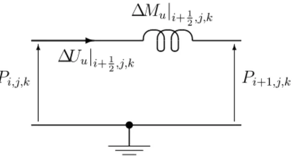
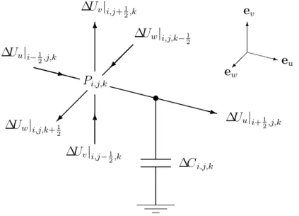
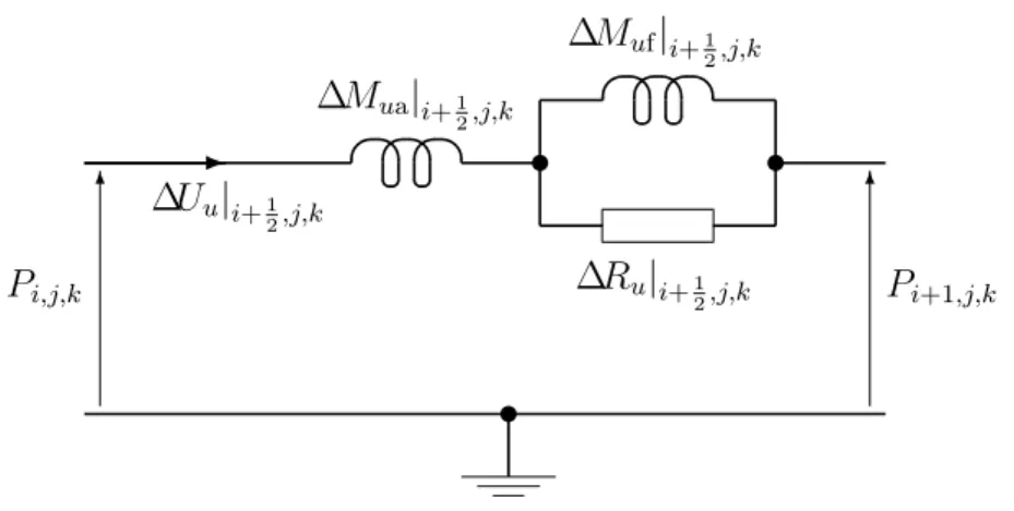
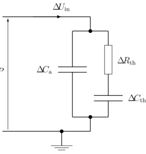
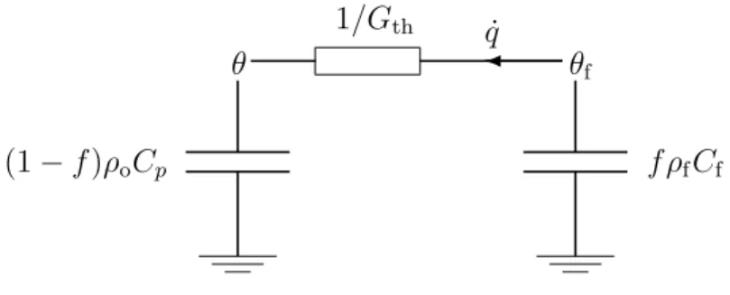
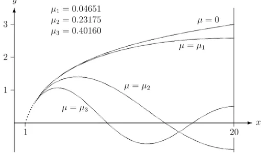
(16) List of Figures 6.1 6.2 6.3 6.4. FDEC FDEC FDEC FDEC. representation representation representation representation. of of of of. Webster’s equation. . . . . . . . . . . . . . . 3D wave equation. . . . . . . . . . . . . . . . equation of motion in u direction, in free air. 3D equation of compression, in free air. . . .. 68 75 77 80. 7.1 FDEC model for equation of motion in u direction, with damping. . . 98 7.2 FDEC model for 3D equation of compression, with damping. . . . . . 110 7.3 Air-fiber heat circuit at constant pressure. . . . . . . . . . . . . . . . 114 8.1. Radial eigenfunctions for m = 20, and limiting function.. . . . . . . . 132. 10.1 Loudspeaker box to be simulated . . . . . . . . . . . . . . . . . . . . 10.2 Equivalent circuit of moving-coil driver connected to time-dependent voltage source vg . . . . . . . . . . . . . . . . . . . . . . . . . . . . . . 10.3 Electroacoustic circuit of Fig. 10.2, with the gyrator remodeled as a bilateral transconductance. Node numbers are also shown. . . . . . . 10.4 Electroacoustic circuit of a moving-coil driver whose diaphragm area is shared between three volume elements . . . . . . . . . . . . . . . . 10.5 Two-dimensional finite-difference equivalent circuit of the interior of the box in Fig. 10.1 . . . . . . . . . . . . . . . . . . . . . . . . . . . . 10.6 Half-space SIL vs. frequency for a 10-inch woofer in a 36-liter box; full simulation. The SIL (sound intensity level) is the IL at one meter, assuming isotropic radiation into half-space and constant parallel radiation resistance. . . . . . . . . . . . . . . . . . . . . . . . . . . . . 10.7 Undamped approximation and full simulation . . . . . . . . . . . . . 10.8 Undamped and lumped approximations . . . . . . . . . . . . . . . . . 10.9 “Free” approximation, for which viscosity is neglected, and full simulation . . . . . . . . . . . . . . . . . . . . . . . . . . . . . . . . . . . 10.10“Unison” approximation, for which the fiber is assumed to move with the air, and full simulation . . . . . . . . . . . . . . . . . . . . . . . . 10.11“Stiff” approximation, for which the fiber is assumed stationary, and full simulation . . . . . . . . . . . . . . . . . . . . . . . . . . . . . . . 10.12Adiabatic approximation and full simulation . . . . . . . . . . . . . . 10.13Thermal-equilibrium approximation and full simulation . . . . . . . . 10.14“Free” approximation and undamped approximation . . . . . . . . . 10.15“Near-adiabatic” approximation, for which ∆Cth is shorted, and full simulation . . . . . . . . . . . . . . . . . . . . . . . . . . . . . . . . . 10.16Full simulation with 25 mm elements and with 50 mm elements . . . . 10.17“Free” approximation with 25 mm elements and with 50 mm elements. xv. 152 157 160 163 165. 171 171 173 174 175 176 177 178 179 180 181 182.

(17) xvi. LIST OF FIGURES 10.18Undamped approximation with 25 mm elements and with 50 mm elements . . . . . . . . . . . . . . . . . . . . . . . . . . . . . . . . . . 10.19Full simulation at 40◦ C and at 20◦ C . . . . . . . . . . . . . . . . . . 10.20Full simulation at an altitude of 1500 meters and at sea level . . . . 10.216.5-inch driver in 5-liter box; adiabatic approximation and full simulation . . . . . . . . . . . . . . . . . . . . . . . . . . . . . . . . . . . 10.226.5-inch driver in 5-liter box; thermal-equilibrium approximation and full simulation . . . . . . . . . . . . . . . . . . . . . . . . . . . . . .. . 183 . 185 . 186 . 187 . 187. 11.1 Normalized FDEC model of a circular rigid-piston source, in cylindrical coordinates . . . . . . . . . . . . . . . . . . . . . . . . . . . . . 201 11.2 FDEC calculation of the transient response at two points in the field of a circular rigid piston in an infinite planar baffle . . . . . . . . . . 211.

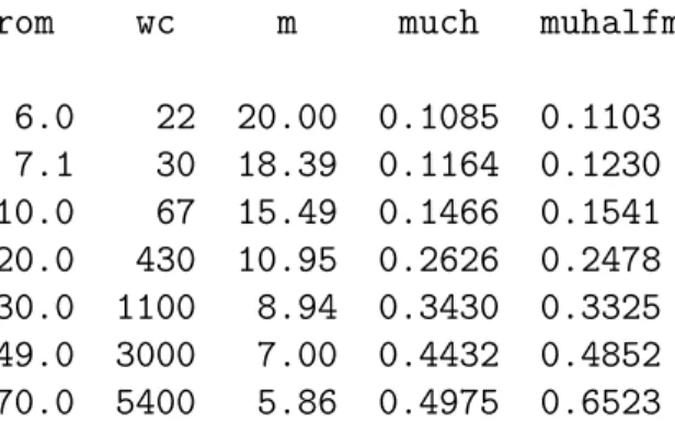
(18) List of Tables 8.1 Algorithm for finding the first three eigenvalues of the radial SturmLiouville problem. . . . . . . . . . . . . . . . . . . . . . . . . . . . . 8.2 Algorithm for checking the calculations of L. M. Chase (1974). . . . 8.3 Check on eigenvalues used by Chase . . . . . . . . . . . . . . . . . . 8.4 Fraction of air volume involved in heat exchange for second mode (right column) vs. filling factor (left column). . . . . . . . . . . . . . 8.5 Algorithm for checking a trial value of ζ in Eqs. (8.15) and (8.67). . 8.6 Errors in analytical approximations to the eigenvalue . . . . . . . . 8.7 Thermal time constant τfp vs. filling factor and fiber diameter . . .. . 131 . 134 . 134 . . . .. 136 137 138 141. 9.1 Computed acoustical properties of air vs. temperature and pressure . 145 11.1 Normalized radiation impedance of a circular rigid piston in an infinite planar baffle, calculated by the FDEC method . . . . . . . . . . 204 11.2 Normalized radiation impedance on one side of an unbaffled circular rigid piston, calculated by the FDEC method . . . . . . . . . . . . . 206. xvii.

(19) Symbols and Abbreviations List of symbols In a thesis containing elements of vector analysis, differential geometry, acoustics, mechanics and thermodynamics, one is likely to encounter different quantities having the same conventional symbol. Reuse of symbols could perhaps be avoided by choosing arbitrary symbols instead of familiar ones, but the reader (not to mention the author) would have trouble remembering the arbitrary meanings. For better or worse, the author has decided to use familiar symbols for familiar quantities, and let some symbols have different meanings in different contexts. Hence some symbols are repeated in the following list. In assigning symbols for related quantities, the following rules have been followed with reasonable consistency: 1. A bold upright character denotes a vector quantity. The same character in an unbold italic typeface, without a subscript, denotes the magnitude of the vector (in a 3D context) or its component in an understood direction (in a 1P context). With a coordinate subscript, it denotes the component in the direction of that coordinate. 2. An alternating time-dependent quantity is denoted by a lower-case italic letter; its phasor form or Fourier transform is denoted by the corresponding capital italic letter. When this is impractical, as when a Greek letter has an upper case that is indistinguishable from an English letter, an underscore is used for the phasor. 3. A subscript “0” indicates an equilibrium value (such as P0 or γo? ), a mean value (ρo ) or a value pertaining to the reference surface Σ0 (Chapter 5). 4. Classical (lumped) acoustic components have a subscript “a” for “acoustic”. This subscript is not used for FDEC elements (which are distinguished by the leading “∆”) unless damping material is involved, in which case the subscript “a” distinguishes the components due to the air alone. 5. An overbar indicates a per-mole quantity. 6. In Chapter 11, normalized values are indicated by lower case (for circuit elements) or a hat (for time-dependent quantities or phasors). The overall arrangement of the following list is alphabetical, ignoring case, with English letters before Greek letters. Logical groups, like the coordinates u, v and w, cause some local variations from this order.. xviii.

(20) xix a b c Ca Cab Cad Cas Cf Cp Cv d eu , ev , . . . f fri fs Gth G h H H, H0 h u , hv , . . . i, j, k k K, K0 Kv , Kw Kv0 , Kw0 m. m ¯ Ma Mab Mad Maf maf Mar mar Mas n n Np p P P0. radius of diaphragm or fiber outer radius of region under study speed of sound, or (with subscripts) normalized compliance element acoustic compliance acoustic compliance of box distributed acoustic compliance (1P) acoustic compliance of suspension mass-specific heat of fiber mass-specific heat at constant pressure mass-specific heat at constant volume fiber diameter unit vectors for coordinates u, v, etc. filling factor (see also ν) relaxation frequency for ith mode free-air resonance frequency of driver air-fiber thermal conductance per unit volume gyrator transconductance (Chapter 10) step size in numerical SLP solution (Chapter 8), or normalized angular frequency (Chapter 11) gyrator transfer resistance (Chapter 10) mean curvatures of Σ and Σ0 (Chapter 5) scale factors for coordinates u, v, etc. Cartesian unit vectors wave number (= ω/c), or a counter in the z direction (Chapter 11) total (Gaussian) curvatures of Σ and Σ0 principal curvatures of surface Σ principal curvatures of surface Σ0 mass (various contexts), or m = f −1/2 = b/a (Chapter 8), or (with subscripts) normalized mass element mean molar mass acoustic mass back air load on driver (FDEC model) distributed acoustic mass (1P), or acoustic mass of driver (no air load) front air load on disk normalized Maf radiation mass normalized Mar acoustic mass of driver (free-air, with air load) amount of gas (moles), or a general-purpose counter unit normal vector to surface neper (dimensionless unit) excess pressure (= pressure rise above P0 ) phasor form of p static (equilibrium) pressure.

(21) xx. SYMBOLS AND ABBREVIATIONS pb pbj pd pdj pf pr Pr Pˆr Pr0 pt q q Q qf Qf Qes , Qms , Qts r R ¯ R r r0 Ra Rar rar Ras Re s S S(ξ) t t0 T T0 Tf u U u, v, w v V Va Vas vg Vg y yn. back pressure on diaphragm (average) back pressure on j th area element developed pressure of driver (average) developed pressure for j th area element front pressure radiated pressure (= pf ) phasor form of pr normalized Pr reference Pr total pressure (= P0 + p) heat energy density (Subsection 7.2.6) air velocity, or heat flux density (Chapter 8) phasor form of q fiber velocity phasor form of qf free-air Q factors of driver (after Small) radial coordinate (cylindrical or spherical) spherical radial coordinate (Chapter 11), or gas constant (mass basis) universal (molar) gas constant position vector (general, or on Σ) position vector on Σ0 acoustic resistance radiation resistance normalized Rar acoustic resistance of suspension resistance of voice coil arc length (more general than ξ) diaphragm area cross-sectional area of ξ-tube unit tangent vector of space curve or of curve on Σ unit tangent of curve on Σ0 instantaneous temperature (K) in Chapter 7; equilibrium temperature (K) elsewhere equilibrium temperature in Chapter 7 temperature of fiber flux (volume velocity) phasor form of u curvilinear orthogonal coordinates specific volume overall volume volume of acoustic compliance suspension equivalent volume terminal voltage phasor form of vg specific acoustic admittance normal specific acoustic admittance.

(22) xxi Za0 Zar zar. reference acoustic impedance (Chapter 11) radiation impedance normalized Zar. α αri. thermal diffusivity absorption coefficient due to ith thermal relaxation mode total absorption coefficient absorption coefficient due to viscosity absorption coefficient due to heat conduction normalized volume-specific heat of fiber ratio of Cp to Cv complex gamma low-frequency limit of γ ? acoustic compliance element adiabatic compliance element thermal relaxation compliance element ∆Cth for infinite-heatsink assumption acoustic mass element (1P) mass element in u direction (other subscripts for other coordinates) air mass element in u direction fiber mass element in u direction thermal relaxation resistance element viscous resistance element in u direction (other subscripts for other coordinates) increment in coordinate u (similarly for other coordinates) phasor flux element (1P); note contrast with ∆u. phasor flux into volume element phasor flux element in u direction (other subscripts for other coordinates) volume element index in formula for τfp (Chapter 8) dynamic viscosity (of air) excess temperature of air, or spherical angular coordinate from polar axis phasor form of θ (excess temperature) initial value of θ (Chapter 8) excess temperature of fiber phasor form of θf thermal conductivity (Chapter 9) vector curvature of space curve (Chapter 5) pneumatic resistivity Sturm-Liouville eigenvalue (Chapter 8) first eigenvalue “rough” analytical estimate of µ1 “refined” analytical estimate of µ1. αt αη ακ β γ γ? γo? ∆C ∆Ca ∆Cth ∆Cth f ∆M ∆Mu ∆Mua ∆Muf ∆Rth ∆Ru ∆u ∆U ∆Uin ∆Uu ∆V ζ η θ Θ θ0 θf Θf κ κ λ µ µ1 µa µb.

(23) xxii. SYMBOLS AND ABBREVIATIONS ν ξ ρ ρo ρe ρe ρf ρ? σ Σ, Σ0 τi τa τfp τfv τp τv φ ψ Ψ ω ωs Ω. kinematic viscosity (Chapter 9), or frequency (Chapter 10) normal arc length coordinate instantaneous density mean density (spatial and temporal) excess density (above equilibrium) phasor form of ρe fiber density (intrinsic glass density) complex density closed surface general constant-ξ surfaces relaxation time for ith mode thermal time constant, constant air temperature thermal time constant, constant Tf and p thermal time constant, constant Tf and v thermal time constant, constant p thermal time constant, constant v angular coordinate common to cylindrical and spherical systems velocity potential phasor form of ψ angular frequency free-air-resonance angular frequency (= 2πfs ) solid angle. List of abbreviations 1P 2D 3D c.d. FDEC FDM HF IL LF ODE OS PDE SIL SLP w.r.t.. one-parameter two-dimensional three-dimensional continuously differentiable finite-difference equivalent-circuit finite-difference method high-frequency intensity level low-frequency ordinary differential equation oblate spheroidal partial differential equation sound intensity level (Chapter 10) Sturm-Liouville problem with respect to.

(24) Chapter 1 Introduction This problem of horns is a “house-on-fire” problem, in the sense that loud speakers are now being manufactured by the thousand, and while they are being manufactured and sold, we are trying to find out their fundamental theory. — Prof. V. Karapetoff [22, p. 405]. Karapetoff was speaking at a convention of the American Institute of Electrical Engineers in 1924. Seventy years later, “loud speakers” are being manufactured by the millions, do not necessarily have horns, and have followed the usual pattern of linguistic evolution by becoming “loudspeakers”—and we are still trying to find out their fundamental theory. Of course there has been spectacular progress along this path. Fourteen months after Karapetoff’s lament came the magisterial paper by Rice and Kellogg [46], showing that a mass-controlled direct-radiating moving-coil transducer could produce a uniform sound-pressure response over a wide frequency range. In later decades, the modeling of moving-coil transducers with enclosures was advanced by Thuras, Olson, Preston, Locanthi, Beranek, Villchur, van Leeuwen, Novak, Thiele, Small, Benson and others (see, for example, the historical notes and original references given by Augspurger [3], Hunt [25, pp. 79–91] and Small [49, 50]). These achievements, together with reasonable criteria for the design of crossover networks, have produced affordable loudspeakers giving tolerably realistic reproduction of sound. In the course of these developments, however, certain issues that one might well regard as “fundamental” have been omitted. The impressive record of progress in other areas makes these omissions all the more conspicuous and surprising, and demands that they be rectified. Karapetoff went on to mention two papers by A. G. Webster, one of which [62] contained a simple differential equation describing the propagation of sound in horns. Webster’s equation, as it is now usually called, must surely be classified as part of the “fundamental theory” of loudspeakers; particular solutions of this equation have inspired a wide variety of horn designs [4], and the properties of its general solutions have been extensively studied [10, 16] with a view to predicting the throat impedance1 of a given horn and hence the frequency response of the driver-horn system. If Webster’s equation is fundamental, so are the assumptions on which it depends. Hence one might ask under what ideal theoretical conditions the equation 1. Acoustic impedance is one of the basic quantities defined in Chapter 2.. 1.

(25) 2. CHAPTER 1. INTRODUCTION. is exactly true, and under what non-ideal practical conditions it is approximately true, in the expectation that these questions had been answered decades ago. It appears, however, that the first reasonably complete and rigorous answers were given in 1993 by the present author [43]. That study, with some subsequent additions and improvements, is presented in Chapters 3 to 5 of this thesis. Another problem that has received surprisingly little attention is the effect of internal resonances in loudspeaker enclosures. The wave-like distribution of pressure inside an enclosure exhibits “modes” or “resonances” at certain frequencies, causing the load on the back of the diaphragm to vary strongly with frequency (calculations and measurements of the impedance presented by a rectangular box were given by Meeker et al. [35] in 1949). This represents a departure from the pure mass-loading prescribed by Rice and Kellogg [46], and consequently causes non-uniform frequency response. The phenomena of resonance and frequency-dependent impedance are unquestionably part of the “fundamental theory” of linear systems, and are usually thought to be theoretically and computationally tractable. But in the field of loudspeaker design, the problem of resonance has been attacked by lining or filling the enclosures with damping material, while the matter of calculating the adverse effects of resonance—with or without the damping—has been largely ignored in the published literature. (Meeker et al. [35] gave a graph of measured box impedance vs. frequency, with and without “sound absorbing lining”, but did not show the effect on frequency response. Sakai et al. [47] gave a very approximate calculation of the effect on frequency response; their work is discussed later.) As is well known, the most successful models of moving-coil loudspeakers in enclosures are based on equivalent circuits. These models have the convenient ability to represent the complete signal path, from electrical input to acoustic output, in a single circuit diagram which can be analyzed using standard computer software. However, all such models that the author has seen in the published literature are lowfrequency approximations developed for the purpose of calculating and optimizing the bass rolloff of the driver. At higher frequencies, these models are misleading because they cannot predict the internal resonances in the enclosure—they allow for the compressibility of the air, and for the contribution of the air to the effective moving mass of the diaphragm at low frequencies, but not for a more complex pressure distribution such as would be capable of representing multiple standingwave modes. An equivalent-circuit model can be modified to account (at least approximately) for the effects of damping materials added in an effort to suppress resonances [30, 49, 50]. However, when the original model is valid only at low frequencies, the version with added damping can do no more than predict the “sideeffects” of damping on the low-frequency rolloff; it cannot predict the degree to which the damping material achieves its primary purpose of suppressing resonances in the midband. These deficiencies can be overcome using the “finite-difference equivalent-circuit” or “FDEC” model, which is the subject of Chapters 6 to 11 of this thesis. If the differential equations describing an acoustic field are approximated by the finitedifference method, the resulting difference equations can be written as the nodal equations of a three-dimensional L-C network. This was shown, for Cartesian and cylindrical coordinates only, by Arai [2] in 1960. In Chapter 6 of this thesis, Arai’s method is shown to be valid for general curvilinear orthogonal coordinates. Chapter 6 also shows how the network can be truncated at the boundaries of the simulated.

(26) 3 region and terminated with additional components to represent a variety of boundary conditions. Chapter 7 shows how the equivalent circuit can be modified to include the mechanical and thermal effects of fibrous damping materials. Chapter 8 obtains an approximate algebraic formula for calculating the thermal time constant between the fiber and the air for constant pressure and constant fiber temperature; one component in each unit-cell of the FDEC model depends on that time constant. The FDEC components also depend on certain properties of air (density, viscosity, thermal diffusivity, etc.), which can be calculated from the temperature and pressure using a set of formulae collected in Chapter 9. In Chapter 10, the results of the preceding chapters are combined with an equivalent-circuit model of a moving-coil transducer to produce a two-dimensional FDEC model predicting the frequency response of a loudspeaker in a fiber-filled box, including the influence of internal resonances. The model can also handle an undamped box, or neglect selected properties of the damping material in order to evaluate the mechanisms of damping. The FDEC model is still a low-frequency approximation, but the highest usable frequency can be made arbitrarily high (given sufficient computational capacity) by making the step size sufficiently small, and is easily made high enough to show a useful number of resonant modes. To show that the FDEC model can accurately represent an anechoic free-air radiation condition at the model boundary, Chapter 11 applies the method to the well-known circular-rigid-piston radiation problem in cylindrical coordinates. The model presented in Chapter 10 is not the world’s first model showing the effect of enclosure resonances on the frequency response of a loudspeaker. Another such model was reported in 1984 by Sakai et al. [47], who used the finite-element method (not to be confused with the finite-difference method used in this thesis) to calculate the acoustic impedance presented by the enclosure to the back of the diaphragm. Sakai et al. went further than the present author in that their model was fully three-dimensional and allowed the shape of a conical diaphragm with a specified semi-apex angle to be accurately represented. They also gave an equivalent-circuit model of the driver and enclosure, incorporating the enclosure impedance. However, instead of solving the circuit with the computed impedance in place, the authors used a mass-limited approximation to the circuit and assumed that the radiated pressure is proportional to the diaphragm acceleration, obtaining a simple formula expressing the sound pressure level in terms of the impedance of the enclosure. The formula was valid only in the midband and discarded the information provided by the equivalent circuit concerning the low-frequency rolloff. Moreover, the assumption of rigid walls together with the neglect of damping in the suspension and pole gap of the driver produced a completely undamped model; hence, at those frequencies for which the reactance of the enclosure canceled the moving mass of the driver, the model predicted an infinite acoustic output. Unlike the model of Sakai et al., the model presented in Chapter 10 always allows for damping in the suspension and consequently does not predict infinite output at any frequency, even for an undamped box. It also allows the modeling of damping due to fiber filling. Whereas Sakai et al. made only temporary use of an equivalent circuit, Chapter 10 of this thesis presents a purely electrical model which places all the capabilities of standard circuit-analysis software, such as SPICE, at the designer’s disposal. (Chapters 10 and 11 assume that the reader has some familiarity with SPICE.) The use of controlled sources in the model allows acoustical quantities.

(27) 4. CHAPTER 1. INTRODUCTION. to be represented without scaling or conversion of units. Electrical quantities are of course also represented literally, so that the model can be immediately extended to account for additional electrical components, such as crossover networks (although this option is not pursued in Chapter 10). Hence, while priority in solving the basic problem is conceded to Sakai et al., the approach adopted in this thesis offers significant advantages.. 1.1. Scope. Any research project is liable to raise more questions than it answers, and consequently will never be “completed” unless some more or less arbitrary limits are imposed on its scope. This is especially the case if the project, like this one, begins on more than one front. But that is not to say that every decision to terminate a particular line of inquiry is arbitrary. Hence a few remarks on the scope of this thesis are in order. In Chapters 6 and 7, the formulae for the FDEC components are expressed in general curvilinear orthogonal coordinates. This decision was motivated by a paper by Geddes [18], which included a discussion of separable coordinate systems and proposed a variety of acoustic waveguides whose walls could be represented as equicoordinate surfaces in suitably chosen coordinate systems; the use of equicoordinate boundaries makes the FDEC method slightly more accurate and much more convenient. Thus the FDEC method is just as applicable to waveguides or horns as to loudspeaker enclosures. Unfortunately it was not opportune to include an analysis of one of Geddes’ waveguides in the long list of contents of the present thesis. It should be noted, however, that the free-air radiation condition modeled in Chapter 11 is a key component in the analysis of any waveguide, and that the FDEC method handles all orthogonal coordinate systems with equal ease provided that the scale factors are known as functions of the coordinates. In other words, this thesis contains sufficient information to enable any interested researcher to undertake a wide-ranging study of exotic waveguides. Of course the limited range of computational examples in this thesis reflects the novelty of the methods, which requires an emphasis on their derivation rather than their application to realistic designs. The absence of a novel waveguide analysis is one illustration. Another is that the loudspeaker models are two-dimensional, with volume elements spanning the full width of the enclosure; one would expect production-quality software to generate fully 3D models, although the 2D treatment in this thesis is a justifiable approximation and yields useful information on the mechanisms of damping while using only modest computational resources. This thesis does not consider all the resonances that might affect the performance of a loudspeaker; it considers aeroacoustic resonances in the cabinet, but neglects structural resonances in the cabinet walls and in the diaphragms and surrounds of the drivers. Structural resonances, like aeroacoustic resonances, can be analyzed by linear approximations, and might therefore be classified as “fundamental”. It may even be possible to include structural deformations in an FDEC model, representing the non-local boundary impedances by means of elaborate patterns of coupled sources. The author has not had time to pursue these issues. However, there is some evidence that structural resonances are—or at least can be made—secondary influences on the performance of practical loudspeakers. The literature reviewed at.

(28) 1.1. SCOPE. 5. the beginning of Section 10.1 suggests that the resonance frequencies of a diaphragm can be kept above the operating frequency range by means of modern materials and structures; suitable structures include honeycomb sandwiches and foam sandwiches, which offer high ratios of flexural stiffness to mass. The same structures can be used in cabinet walls to keep their resonance frequencies high [57, p. 229]. Lipschitz et al. [32] have computed the radiation from the walls of several loudspeaker cabinets, using measurements of the wall vibrations. Their results indicate that, even with conventional wooden construction, variations in frequency response due to cabinet wall vibrations can be reduced below the level of audibility, provided that the cabinet includes adequate internal bracing.2 The “ripples” in the frequency response of a typical high-quality loudspeaker may amount to several dB, which is more than can be accounted for by any of the results obtained by Lipschitz et al. In summary, structural resonances have received more attention in the literature than aeroacoustic resonances, and the results suggest that structural resonances need not be a major influence on performance. The comparative shortage of literature on aeroacoustic resonances and the influence of damping materials, together with the comparative ease with which these questions can be tackled by equivalent-circuit methods, supports the decision to study only aeroacoustic resonances in this thesis. Other resonances may be considered in future work.. 2. Of course, careless design of the cabinet may produce objectionable resonances. Barlow [7] has investigated structural resonances in various loudspeaker components; he reports that in some cases, sound radiation from resonating cabinet walls can exceed the radiation from the driver. But the findings of Tappan and Lipschitz et al. convince the present author that such problems are readily preventable..

(29) Chapter 2 Foundations While this chapter contains material that can be found in undergraduate textbooks on acoustics, it also presents the one-parameter (1P) forms of the equations of motion and compression, a rigorous derivation of electrical-acoustical analogs (including the justification for connecting the analogous components to form circuits), and a unified discussion of linearizing approximations, including the neglect of gravity. Such issues cannot be discussed in isolation from the most elementary theory. Hence an introductory chapter presenting only the original material while quoting the rest from textbooks, if it were possible at all, would be incoherent. Moreover, acoustics textbooks tend to derive the equation of motion and the equations of continuity and compression in an ad hoc manner, assuming a specific coordinate system and without exploiting the machinery of vector analysis. The textbook approach accommodates readers with modest mathematical background, but would not be appropriate here because its lack of generality would lead to needless repetition and loss of logical continuity, thus obscuring the close interdependence of the results. The approach adopted here is to begin with the most general form of each equation, then obtain the other forms by successive specialization. Among the advantages of this discipline are the following: • Repetition of mathematical steps is avoided; • Each approximation or assumption is made only once, not only saving time, but also showing clearly which results depend on which assumptions; • The generality of the results is maximized (for example, the first formula for the acoustic mass of a port does not assume a uniform cross-section); • The common theoretical foundation provides some intuitive rationale for the results of later chapters (for example, the expressions for the components of the finite-difference equivalent circuit in Chapter 6 will have familiar forms, and will seem plausible). Finally, as this thesis is nominally in the discipline of electrical engineering, one measure of its merit is its potential to attract electrical engineers into the field of electroacoustics. That potential will be enhanced if the thesis serves as its own introduction to any necessary theory that is not part of the standard training of electrical engineers. Such is the theory presented in this chapter.. 6.

(30) 2.1. FORMS OF THE EQUATION OF MOTION. 2.1. 7. Forms of the equation of motion. The equation of motion expresses Newton’s second law for a non-viscous fluid. It will be derived first in its most general integral form, then reduced to a point form valid for irrotational flow, low gravity and small oscillations and compressions. The point form is integrated to give a “one-parameter” or “1P” form, which applies to normal oscillations of a uniform thin shell of the fluid and is useful in the analysis of horns and ducts. This in turn is integrated to give a fourth form applicable to ports or vents (mass elements) in loudspeaker boxes. Note that each form of the equation will inherit all the assumptions contained in the previous form.. 2.1.1. Integral form. In a non-viscous fluid, let σ be a simple closed surface moving with the fluid. Let dσ denote the element of surface area and n the (outward) unit normal to σ. Let the three-dimensional region enclosed by σ be called V, with every differential volume element dV also moving with the fluid. Each volume element will then contain a constant mass dm = ρ dV, where ρ is the density. Let pt be the total instantaneous pressure and q the instantaneous velocity (q is a vector; in this thesis, unless otherwise noted, symbols representing vector quantities will be in bold, upright type). In general ρ, pt and q will depend on position and time. Let g be the local acceleration due to gravity, which is assumed to be the only external force (“body force”) acting on the fluid. Newton’s second law for the enclosed sample of fluid is d (total momentum) = total force, dt. (2.1). i.e.. ZZZ ZZ d ZZZ q dm = (2.2) g dm − pt n dσ , dt V V σ where the first integral on the right is the weight of the enclosed fluid, and the signed second integral is the force exerted by the pressure of the surrounding fluid (the sign is negative because each element of this force is in the direction of −n).. 2.1.2. Differential or point form. The right-hand term in Eq. (2.2) can be expressed as a volume integral using the gradient theorem [24, pp. 141–2] and rewritten in terms of mass elements, as follows: ZZ. pt n dσ = σ. ZZZ. V. ∇pt dV =. ZZZ. V. ∇pt dm. ρ. (2.3). !. (2.4). This may be substituted into Eq. (2.2) to obtain . ZZZ d ZZZ ∇pt q dm = dm. g− dt V ρ V. Let us treat dm as a small mass contained in the small volume dV, so that the volume integral represents a summation. Then, since the above equation holds for all volumes moving with the fluid, it applies to each volume element dV. For each.

(31) 8. CHAPTER 2. FOUNDATIONS. element there is only one term in the “summation”, so that the above result reduces to Euler’s equation1 : 1 dq = g − ∇pt . (2.5) dt ρ Euler’s equation expresses Newton’s second law at a point moving with the fluid, so that dq/dt is the acceleration of a single particle of the fluid. Hence the convention in fluid mechanics that the total derivative of a function with respect to (w.r.t.) time is evaluated at a point moving with the fluid, while the corresponding partial derivative is evaluated at a stationary point. Since the partial derivative will prove easier to work with, it is desirable to rewrite Euler’s equation in terms of ∂q/∂t. In Cartesian coordinates, from the chain rule for partial derivatives, we have ∂q ∂q dx ∂q dy ∂q dz dq = + + + dt ∂t ∂x dt ∂y dt ∂z dt ∂q ∂q ∂q ∂q = + qx + qy + qz ∂t ∂x ∂y ∂z ∂q = + (q.∇)q ∂t. (2.6). where qx , qy and qz are the components of q in the directions of i, j and k (cf. Hsu [24], pp. 222–3). We now introduce the vector identity2 (q.∇)q = 12 ∇(q.q) − q × (curl q). (2.7). and write |q| = q, so that q.q = q 2 . Substituting all this into Eq. (2.6) yields the general relationship between dq/dt and ∂q/∂t in coordinate-independent form: dq ∂q 1 = + 2 ∇(q 2 ) − q × (curl q). dt ∂t. (2.8). Substituting this into Eq. (2.5), and adopting the convention—to be followed in the remainder of this thesis—that a dot denotes partial differentiation w.r.t. time, we obtain Euler’s equation in terms of q˙ = ∂q/∂t: q˙ + 12 ∇(q 2 ) − q × (curl q) = g −. 1 ∇pt . ρ. (2.9). Thus the general form of Euler’s equation—which assumes only that the fluid is non-viscous—is nonlinear in q and ρ (note the q 2 and 1/ρ factors) and nonhomogeneous (the terms contain unlike powers of the dependent variables). This rules out superposition and all solution methods that follow therefrom, including separation of variables and integration of Green’s functions. To linearize and homogenize the equation, we make the following approximations: • The flow is irrotational ; that is, curl q = 0, so that one nonlinear term is eliminated from Eq. (2.9). 1. Euler’s equation may also be obtained by moving the d/dt operator inside the volume integral, as in Hsu [24], pp. 216–7. 2 Hsu [24, pp. 111, 223] derives identity (2.7) by an unusual operational method. A more conventional approach is to use Cartesian coordinates and show that the i components of both sides are equal; the j and k components behave similarly..

(32) 2.1. FORMS OF THE EQUATION OF MOTION. 9. • Oscillations are small; that is, q is small. The first term is Eq. (2.9) is linear in q while the next two terms are quadratic in q. Hence, if q is sufficiently small, the second and third terms will be negligible compared with the first. We do not yet know how small is “sufficiently small”, although this can always be checked by calculating the first and second terms after an approximate solution has been found (see e.g. Ballantine [4], pp. 88–9). The meaning of “small oscillations” will be clarified in Subsection 2.4.1. Also note that the irrotational-flow assumption seems to have been made redundant, since the small-oscillations assumption makes the term containing curl q negligible. This issue will be taken up again in Subsection 2.3.1. • The external force per unit mass is conservative—which is certainly the case for gravity. Hence g has a potential function: let g = −∇V.. (2.10). • Compressions are small; that is, all spatial and temporal variations in ρ are small compared with its mean value. This applies not only to variations caused by excitation of the fluid, but also to those caused by the gravitational pressure gradient—this is the low-gravity assumption. Thus we can write ρ ≈ ρo ,. (2.11). where ρo is the mean density. The above substitution linearizes the last term in Eq. (2.9) and, when combined with Eq. (2.10), allows the right side of Eq. (2.9) to be written as a single gradient. After the above approximations and substitutions, Eq. (2.9) becomes q˙ = −. 1 ∇(pt + ρo V ) ρo. (2.12). which is much simpler than the exact form. But because of the ρo V term, this result is still inhomogeneous in pt and q. (That is, if we have a solution (pt ,q), we do not obtain another solution by multiplying pt and q by an arbitrary constant α, unless ∇V = 0; for a proof, replace pt and q in Eq. (2.12) by αpt and αq, then subtract α times Eq. (2.12).) We can homogenize Eq. (2.12) by rewriting it in terms of the excess pressure, denoted by p, which is the pressure rise above equilibrium. Let the equilibrium pressure be P0 (note that P0 is a function of position, although ρo is not). Then the excess pressure is p = pt − P0 . (2.13).

(33) 10. CHAPTER 2. FOUNDATIONS. For the equilibrium condition, we put q˙ = 0 and pt = P0 in Eq. (2.12) and find3 0=−. 1 ∇(P0 + ρo V ). ρo. (2.14). Subtracting this from Eq. (2.12), and using Eq. (2.13) to write the result in terms of p, we obtain the desired linear homogeneous form: q˙ = −. 2.1.3. 1 ∇p. ρo. (2.15). One-parameter or thin-shell form. A third form of the equation of motion assumes a one-parameter (1P) distribution of pressure; that is, it assumes that the excess pressure p is a function of time and of a single spatial coordinate ξ, whose level surfaces may in general be curved. To facilitate concise discussion, the following terminology will be used throughout this thesis: ξ-surface: surface of constant ξ; ξ-trajectory: orthogonal trajectory to the ξ-surfaces; ξ-tube: tube of ξ-trajectories, i.e. the surface generated by all the ξtrajectories intersecting a simple closed curve contained in a ξsurface; ξ-shell: three-dimensional region between two infinitesimally close ξsurfaces; ξ-shell segment: three-dimensional region bounded by two infinitesimally close ξ-surfaces and a ξ-tube. The 1P form of the equation of motion also assumes that ξ is an arc-length coordinate, i.e. that the ξ coordinate of a point R is the directed arc length along the ξ-trajectory from the surface ξ = 0 to the point R.4 Familiar examples of arc-length coordinates are the three Cartesian coordinates and the radial coordinates in the cylindrical and spherical coordinate systems. For some examples of the mathematical objects defined above, we may replace ξ with the radial coordinate r in the 3. For interest’s sake, and for a check on the preceding work, we can use Eq. (2.14) to find the equilibrium pressure P0 . Since a function of position with zero gradient is constant, we see that P0 + ρo V is equal to a constant, say Pm . Then P0 = Pm − ρo V. If g is the acceleration due to gravity, we can take a Cartesian coordinate system with the z axis pointing upward and write g = −gk, for which a potential function is V = gz. The equilibrium pressure then becomes P0 = Pm − ρo gz which shows the familiar variation of hydrostatic pressure with height. 4 It will be shown in Chapter 4 that if p depends on only one spatial coordinate, that coordinate can be transformed to an arc-length coordinate. Hence the second assumption is redundant. In Chapter 5, it is further shown that the orthogonal trajectories to the level surfaces of an arc-length coordinate are straight lines; this justifies the assumed existence of ξ-tubes. For the moment, however, the single-coordinate assumption and the arc-length assumption will be treated as independent hypotheses, and the existence of ξ-tubes will be regarded as self-evident..