Correcting Motion Distortions in Time-of-Flight Imaging

HAL Id: hal-01890418

https://hal.archives-ouvertes.fr/hal-01890418

Submitted on 8 Oct 2018

HAL is a multi-disciplinary open access

archive for the deposit and dissemination of

sci-entific research documents, whether they are

pub-lished or not. The documents may come from

teaching and research institutions in France or

abroad, or from public or private research centers.

L’archive ouverte pluridisciplinaire HAL, est

destinée au dépôt et à la diffusion de documents

scientifiques de niveau recherche, publiés ou non,

émanant des établissements d’enseignement et de

recherche français ou étrangers, des laboratoires

publics ou privés.

Correcting Motion Distortions in Time-of-Flight Imaging

Beatrix-Emöke Fülöp-Balogh, Nicolas Bonneel, Julie Digne

To cite this version:

Beatrix-Emöke Fülöp-Balogh, Nicolas Bonneel, Julie Digne. Correcting Motion Distortions in

Time-of-Flight Imaging. Motion, Interaction and Games 2018, Nov 2018, Limassol, Cyprus. pp.no 8,

�10.1145/3274247.3274512�. �hal-01890418�

Beatrix-Emőke Fülöp-Balogh

Nicolas Bonneel

Julie Digne

ABSTRACT

Time-of-flight point cloud acquisition systems have grown in preci-sion and robustness over the past few years. However, even subtle motion can induce significant distortions due to the long acquisition time. In contrast, there exists sensors that produce depth maps at a higher frame rate, but they suffer from low resolution and accuracy. In this paper, we correct distortions produced by small motions in time-of-flight acquisitions and even output a corrected animated sequence by combining a slow but high-resolution time-of-flight LiDAR system and a fast but low-resolution consumer depth sensor. We cast the problem as a curve-to-volume registration, by seeing a LiDAR point cloud as a curve in a 4-dimensional spacetime and the captured low-resolution depth video as a 4-dimensional spacetime volume. Our approach starts by registering both captured sequences in 4D, in a coarse-to-fine approach. It then computes an optical flow between the low-resolution frames and finally transfers high-resolution details by advecting along the flow. We demonstrate the efficiency of our approach on both synthetic data, on which we can compute registration errors, and real data.

CCS CONCEPTS

• Computing methodologies → 3D imaging; Motion capture; Point-based models;

KEYWORDS

3D Video, Dynamic Point Sets, Detail transfer

ACM Reference Format:

Beatrix-Emőke Fülöp-Balogh, Nicolas Bonneel, and Julie Digne. 2018. Cor-recting Motion Distortions in Time-of-Flight Imaging. In MIG ’18: Motion, Interaction and Games (MIG ’18), November 8–10, 2018, Limassol, Cyprus. ACM, New York, NY, USA, 7 pages. https://doi.org/10.1145/3274247.3274512

1

INTRODUCTION

Capturing accurate 3D geometries is a powerful way for artists to design sceneries, for historians to reconstruct old monuments, for real-estate agents to communicate their products or for nav-igation systems to provide context. It has become a widespread need, and, when it comes to static environments, is now mostly sucessfully performed using laser technologies such as LiDaR, that capture environments at sub-millimeter accuracy. When it comes to slightly moving, let alone fully animated scenes, this technology breaks. In fact, capturing a single frame can take tens of seconds,

Permission to make digital or hard copies of all or part of this work for personal or classroom use is granted without fee provided that copies are not made or distributed for profit or commercial advantage and that copies bear this notice and the full citation on the first page. Copyrights for components of this work owned by others than the author(s) must be honored. Abstracting with credit is permitted. To copy otherwise, or republish, to post on servers or to redistribute to lists, requires prior specific permission and/or a fee. Request permissions from [email protected].

MIG ’18, November 8–10, 2018, Limassol, Cyprus

© 2018 Copyright held by the owner/author(s). Publication rights licensed to ACM. ACM ISBN 978-1-4503-6015-9/18/11.

https://doi.org/10.1145/3274247.3274512

Kinect frame 326 frame 442 frame 529

Lidar scan Corrected scan

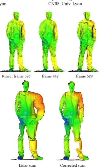
Figure 1: A consumer depth sensor acquires dense low-resolution scans at a high rate (top row) while a LiDaR scan-ner acquires sparse high resolution scans containing time distorsions (bottom left). We recover details by undistorting the LiDaR scan (bottom right).

which makes any motion problematic. Even small motions manifest as distortions (Fig. 1) altering the reconstructed point cloud. For dynamic scenes, one often resorts to much less accurate systems such as infrared sensors (Microsoft Kinect or Creative Senz3D), or structure-from-motion using multiple video cameras. These sys-tems allow for capturing rough depth of an entire field of view at 30-60 frames per second, albeit at low resolution, with an accu-racy of centimeters and numerous outliers. These setups gained popularity with interactive console 3D games for which neither precision nor accuracy is crucial. For accurate dynamic scene recon-struction, no satisfactory solutions exist and one often resorts to high-resolution templates deformed to match rough motions. This

MIG ’18, November 8–10, 2018, Limassol, Cyprus B. Fulop-Balogh et al.

is particularly the case for facial animation, but does not generalize well to different geometries.

In this paper, we provide the insight that using both laser and infrared technologies at the same time, one can undistort and partly recover a more accurate geometry in the presence of moderate motions. We design a method that registers an accurate LiDaR point cloud captured at a low temporal framerate to a coarse spatio-temporal depth-sensor point cloud captured at interactive framerate, without any preliminary device cross-calibration. We formulate this problem as a spacetime curve-to-volume rigid correspondence prob-lem efficiently solved using a Hough transform and Iterative Closest Point algorithm. Our intuition is that, due to the capture time, a LiDAR point cloud can be seen as a curve in a 4-dimensional space-time, in which points are each identified by a single (x,y, z, t) value, while a real-time depth video camera produces (x,y, z) dense slices for individual timestamps at a high frame-rate, resulting in a sliced 4-dimensional spacetime volume. We then transfer details from the LiDaR to the Kinect point cloud and advect them across frames, leading to a detailed animated model. We validate our method on synthetic data, and demonstrate it by recovering high-resolution dynamic geometries under moderate motion.

2

RELATED WORK

Acquisition of high resolution dynamic shapes. has been tackled using stereo and active light projection systems [Koninckx and Gool 2006], such as fringe projection and time shifting [Zhang 2010]. In the special case of facial motion capture, Zhang et al. [2004] propose to use synchronized video cameras and structured light projector and fit a highly detailed template to the resulting geome-try to get a high resolution facial animation. Bradley et al. [2010] avoids templates by using a high-resolution multi-camera setup to reconstruct detailed facial geometry. Weise et al. [Weise et al. 2011] use a consumer depth sensor to animate a face template. A combination of active light and stereo was also proposed for cap-turing scenes in real time with motion compensation [Weise et al. 2007]. More generally, high spacetime resolution capture can be performed using multiview stereo techniques [Davis et al. 2005; Zhang et al. 2003]. Yet the resolution is often limited, depending on the number of views and size of captured objects. Sensors also need synchronization and often, heavy calibration, which can make them difficult to use in practice.

Static point set super-resolution. has been tackled by Kil et al. [2006] where several nearby scans are registered and merged together to obtain a high resolution point cloud. More recently, Hamdi-Cherif et al. [2018] nonlocally merge self similar patches of a LiDaR scan to improve its resolution. In a quite different setting, Haefner et al. [2018] proposed to perform single frame super-resolution from a kinect scan by using shape from shading to solve this ill-posed problem.

Texture synthesis and transfer. High resolution and detailed ani-mations synthesis is a hot topic in computer generated animation research. Rohmer et al. [2010] generate detailed wrinkles on an animated mesh to make it look more realistic, Bertiken et al. [2017] propose a way to transfer details from similar areas of one shape to another, using metric learning.

Enhancing Videos with stills. Our method share similarities with the problem of enhancing a low-quality video with high resolution stills. The main difference is that no motion-induced geometric distorsions appear in still photography whereas rolling-shutter-like distorsions are accounted for in our LiDaR point cloud. The video enhancement problem bas been tackled by considering a spacetime volume of (x,y, t) pixel coordinates. In that space, a video is a sub-volume, while a still photography is a plane. By aligning videos and stills in that volume [Caspi and Irani 2002], Shechtman et al. [2005] merge the information from these two sources and increase space-time resolution. Liu et al. [2014] improve the spacespace-time resolution using a sparse decomposition on a pre-learned dictionary. When the scene is static, Bhat et al. [2007] use structure-from-motion to reconstruct a 3D proxy from the video. Then for each frame, the best still photograph is selected and used to improve the video using image-based rendering and Markov Random Fields. Similarly Gupta et al. [2008] enhance a video by selecting pixels from neigh-boring high-resolution stills using a graph-cut formulation. Ancuti et al. [2010] proposed a Maximum a Posteriori-based modeling of this problem that is also limited to static scenes.

3

OVERVIEW

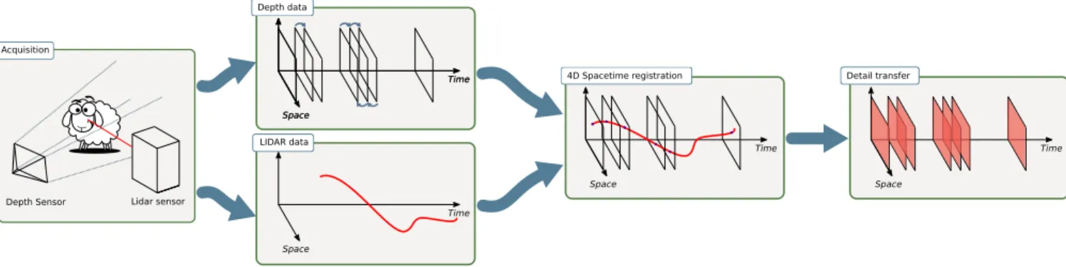
As input, our method takes two 3D point clouds of the same dynamic scene, under small to moderate motion: a set of low-resolution point clouds obtained at 30fps from a structured-light infrared depth sen-sor (such as Kinect) during the motion, and a single accurate but distorted time-of-flight laser LiDaR point cloud taken during the same period of time. While the former provides a low-resolution point set at regular time intervals, the latter provides a highly accu-rate point set but at a single time stampt for each point. We will refer to the structured-light frames as LR frames, and similarly, to the time-of-flight data as HR data. In practice, both setups capture depth values of the scene with respect to the device. Due to motion in the captured scene, the HR point cloud appears distorted (Figure 1) but each point is precisely captured. The LR frames do not suf-fer from such time-distortion but exhibit a poor quality: spatially inaccurate and quantized depth values with large noise at a low 0.3 mega-pixel resolution. Our core idea is thus to un-distort the HR data that is accurate in space based on the motion captured by the LR data that is accurate in time. The process if summarized in Figure 2.

Our goal is to resample HR points in time to obtain a high-resolution point set for each time frame. This is achieved through three steps. First, we estimate a motion field between the depth sensor LR frames using an off-the-shelf RGB-D optical flow tech-nique. Second, we observe that, up to missing data and noise, the HR point cloud can be exactly registered to the LR data via a rigid transform. In the 4D spacetime continuum, we see the LR frames as a set of 3D spatial “slices” taken at regular time intervals, while the HR point cloud is seen as a time-parameterized curve in the 4D volume as each captured 3D point corresponds to a unique time stamp (Figure 2). This registration step hence amounts to finding a curve pattern within a 4D volume. We robustly perform this step using a global Iterative Closest Point algorithm initialized via an adaptation of a coarse generalized Hough transform. Finally, we

Space Time Space Time Space Time Space Time 4D Spacetime registration Depth data LIDAR data Detail transfer Space Time Acquisition

Depth Sensor Lidar sensor

Figure 2: Overview of our high resolution dynamic point set acquisition and processing algorithm

use the motion field to advect details from the registered HR data across depth sensor frames.

4

SCENE FLOW ESTIMATION

To be able to transfer details from the time-of-flight HR acquisition to the LR depth video frames, it is necessary to track 3D points of the LR depth frames through time. A solution to this problem would be to work solely on the depth information and use an al-gorithm to register Dynamic Point Sets without computing point to point correspondences [Mitra et al. 2007]. However, in our case, the depth sensor provides color information which, if properly reg-istered to the depth frames, gives valuable information. The flow obtained from RGBD images is called scene flow. It is a variant of the more common optical flow between color images (e.g. [Fleet and Weiss 2006]), with the additional challenge that the flow should also account for depth information, and not only the color. In recent years, several approaches have been proposed to solve this problem (e.g. [Herbst et al. 2013; Huguet and Devernay 2007; Quiroga et al. 2014]). We use the approach of Quiroga et al. [2014] that extends variational optical flow estimation from color image sequences to RGBD videos. This method favors a piecewise smooth scene flow by modeling motions as twists and introducing a total variation regularization.

The computed scene flow provides a way to track a point across all frames until the end of the sequence or until it becomes occluded. It will later be used to advect details from the HR dataset.

5

REGISTRATION IN THE 4D SPACE

In the 4-dimensional spacetime volume, the LR data provides a set of regularly spaced 3D hyperplanes while HR data provides a single curve parameterized by the timet (see Section 3). We adopt a two-step procedure to align the curve to the 3D hyperplanes. We see this operation as the problem of searching for a pattern within a point cloud. We initialize this search using a coarse, discretized, Hough transform, which we fine-tune in a second step using an ICP. Because of efficiency concerns, we first register the data in the 3D space only, disregarding the time component completely, where we interpret the two point clouds as their projections along the time axis to the 3D space. Then, we perform both the coarse and fine registration steps again, this time on 4-dimensional point sets. This section describes these steps in more details.

5.1

Problem formulation

If both the LR and HR sensors are located at the same place, share the exact same field of view and the capture starts at the same time t0, then all captured points are completely aligned in spacetime and

share the same spacetime coordinate frame. However, this is never the case as both cameras capture different portions of the scene and are hard to synchronize. In addition, the raw HR data do not directly include a time-stamp for each captured 3D point, instead we roughly estimate the time-stamp using the total acquisition time and the scanline pattern of the acquisition. The first operation we perform is thus a registration procedure that brings both datasets to the same space. This amounts to estimating a rotation and translation in space, together with some translation and possible scale in time, to match one dataset to the other. Moreover, due to the inaccuracy of the LR frames, adjusting a scale in space is also necessary for a good alignment. The whole registration thus corresponds to the search for a single global 3D spatial rotationR = (θx, θy, θz), a 4D spacetime translationT = (Ts, tt) and a 4D spacetime scale s = (ss, st).

We parameterizeR by three Euler angles, the translation Ts by three coordinates, andtt,ss andstare three scalars. This registra-tion procedure amounts to estimating 9 parameters. We will denote the entire 9-d transformation T. Denoting H the HR point set (resp. L the low-resolution structured light data) in 4D, we formulate the registration problem as the minimization:

min

T

Õ

p

∥Tp − q∥2_,

wherep ∈ H and q ∈ L is the closest LR point to p.

5.2

Coarse initialization

Rough estimates of these parameters can be obtained using a voting scheme akin to the generalized Hough transform traditionally used for detecting shapes in images, by discretizing a well-chosen pa-rameter space, and computing the scores of each set of papa-rameters. Historically, the Hough transform was first introduced to detect straight lines on images by discretizing line parameters and scoring them [Duda and Hart 1972]. It was later extended to more general shapes by discretizing a space of shape template transforms [Ballard 1981].

MIG ’18, November 8–10, 2018, Limassol, Cyprus B. Fulop-Balogh et al.

In our case, we detect our HR curve on the LR volume by dis-cretizing the 9-dimensional space of transformation parameters described in Sec. 5.1. However, given the sheer amount of data and the curse of dimensionality affecting our 9-dimensional space, some adaptations are needed.

First, it’s easy to see that by placing both the consumer depth sensor and the LiDaR system in an upright position facing the scene θxandθz become negligibly small for the purpose of the coarse registration step, so they can be safely omitted. Then, scaling in space is only included to make up for the inaccuracy of the LR data and thus it should be close enough to 1 not to alter the results of the Hough Transform applied at such a low resolution. Considering these observations the 9-dimensional parameter space P is first safely reduced to a 6-dimensional space P′.

As mentioned previously, the registration procedure is divided into an initial phase computing only the transformation Tsin space and a final one computing the translationttand scalestin time. In the context of the Hough Transform this means that P′can be further divided into two separate parameter spaces Ps(θ_y, t_x, t_y, t_z) and Pt(t_t, s_t) which are discretized at a given resolution.

For each set of parameters of the form Ts = (θy, tx, ty, tz) and Tt = (tt, st), corresponding to a bin in Ps and Pt respectively, we compute a score which represents how well the transformed point cloud TsH in space and TtH in 4D spacetime are registered to L and seek to maximize it. When working on Ps, the LR data is converted, at a given rough resolution ˜L, to a voxel grid VL˜

with each voxel v storing the number of points lying in it. Then the HR data is transformed using Ts and discretized into a grid V



TsHusing the same resolution as ˜L. The score of Tsis computed

asÍ

vmin(VL˜(v), VTsH(v)). The final solution is found as the

transformation Tswith the highest score.

In the case of time registration, 4-dimensional voxels would not allow a high enough resolution neither in the parameter space Pt

nor for the voxel box. Our alternative solution is to search for a transformation Ttthat minimizes the point-wise distance between TtH and L.

5.3

Fine registration

The solution of the coarse registration step is only known up to the precision of the parameter space discretization. This is insufficient as we aim at transferring millimeter-scale details. Hence, in a second step, we refine the rough estimate both in the 3D case first and then in the 4D spacetime. As the coarse solution is assumed to be close to the optimal solution, we can now resort to a local optimization, namely an ICP [Besl and McKay 1992], to refine T. Let H′= TH, the new transformation T′is found by iterating the classical two steps: 1) assign to each pointpi ∈ H′its closest pointqi ∈ L (if no point is found closer to a given threshold then the point is simply omitted). 2) Find the transform T′minimizing:

Õ

i

∥T′pi−q_i∥2,

which is solved using Kabsch algorithm for the translation in 4D and rotation in space. The scale in time is solved by computing the standard deviation of the time stamps of the matched pointsσp

andσqof H′and L and deriving the scale asss =σσqp. Conversely,

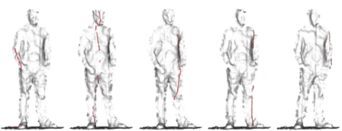
Figure 3: Registration result. For 5 different time valuest, we select LR and HR points that lie in a small temporal neigh-borhood after the spacetime registration. The LR points are oriented and displayed in grayscale values while the HR points are shown in red. The LiDAR scanline acquisition pro-cess results in vertical lines.

the scale in space is computed by averaging the ratios of the 3D Eu-clidean distances between HR point pairs and their LR counterparts as follows: ss = _|H1′_|2 Õ i, j ∥p_i−p_j∥ ∥qi−q_j∥.

At the end of the iterations the HR pointspiwith no sufficiently close LR counterpartqiare considered occluded from the point of view of the LR sensor and are discarded.

The result of the spacetime registration can be seen in Figure 3: for different time valuest, we display the LR and HR points that lie in a small temporal neighborhood aroundt, showing that our spacetime registration matches well the datasets despite the difference in resolution.

6

DETAIL TRANSFER

Now that both the high and low resolution point clouds share the same spacetime coordinate frame, the last step of our algorithm advects the HR point cloud to enrich all frames of the LR point cloud. To do so, we rely on our estimate of the scene flow between consecutive LR frames (see Section 4), and advect HR points accord-ingly.

Let us consider a pointp ∈ H and Ft its closest LR frame in time. A search in the 3D space findsQ_pt ⊂ Ft as the set of its nearest neighbors in framet. The motion estimated at each point qt_i ∈Qt_pis then interpolated in space and time to bringp to the exact timestampt of Ft. Nextp is advanced by one frame in time based on the scene flow of the pointsQ_pt. This process is performed iteratively until no sufficiently close nearest neighbor can be found which meansp is occluded.

7

RESULTS

We validate our approach using two datasets. First, using synthetic data, we make sure our method allows to transfer details with sufficient accuracy, and evaluate any reconstruction error. Second, we showcase our method on real data and show it to be of sufficient accuracy to be used to undistort small to moderate motions.

LiDaR scan LR frame (1) (2) (3) (4) Ground truth

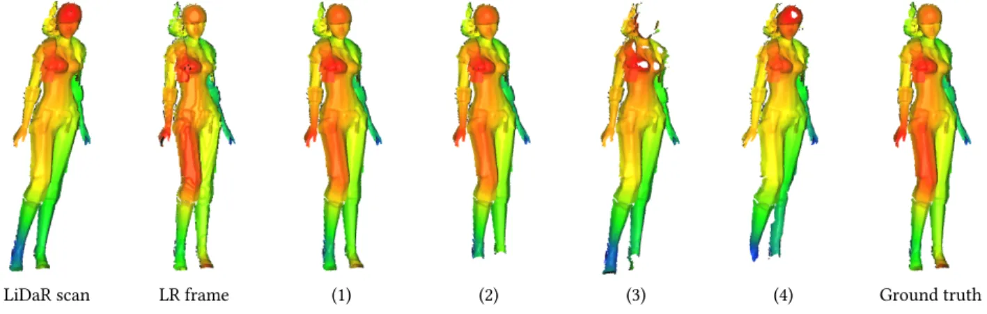
Figure 4: Synthetic dataset along with reconstructed frames for validating various steps of our method as described in Table 1

Table 1: Average point-wise distances between reconstructed and generated ground truth point clouds using either known (GT) registration parameters and motion field or computing them using our method (E). All errors are below 2% of the shape height (2.5 units)

Used methods Distance GT registration and GT motion field (1) 0.01271 E registration and GT motion field (2) 0.01463 GT registration and E motion field (3) 0.04368 E registration and E motion field (4) 0.04479

7.1

Simulated Data

Our simulated data consists of a single character undergoing a rigid transformation T= (Ts, Rs), raytraced from different viewpoints using parameters similar to LR and HR devices. This synthetic data allows us to synthesize a distortion-free dynamic point set, serving as a groundtruth, and compare our result to it.

To simulate the noise introduced by the commercial depth sen-sor we generated depth-bins increasing in size proportionally to the distance from the camera mimicking the quantization errors introduced by the sensor and matched the computed depth values to the depth-bins. However we do not simulate any depth sensor calibration error.

Table 1 shows the accuracy of the different steps of our method. By using the known values of the parameters of the 4D registration and the precomputed motion field we assess separately the noise introduced only by the detail transfer. On the contrary, by using no prior knowledge of the scene the average distances indicate the accumulated error introduced throughout the steps of our method. Figure 4 shows the reconstructed frames along with the ground truth of a dataset.

7.2

Real Data

We now turn to the more difficult case of real data. Our experi-mental setup is the following. A LiDaR and an ASUS Xtion sensor acquire the same animated scene yielding respectively a high reso-lution depth data (corresponding to H ) and a low-resoreso-lution dense

Figure 5: Our experimental setup: a Kinect and a LiDaR ac-quire the same scene from different viewpoints. No calibra-tion is required.

depth video (corresponding to L). Our system does not require any manual calibration: both acquisition systems are only roughly synchronized and we only need them to start roughly at the same time (in practice, the Asus depth sensor capture often starts several seconds before the LiDaR as the LiDaR performs an automatic self-calibration procedure at the start of each capture). A picture of the acquisition system is shown on Figure 5.

The Xtion captor. captures 30 depth frames per second with a resolution of 640 × 480, the capture is performed using the OpenNi 2 library [organization 2017], removing distortion and yielding the final 4D point cloud in millimeters and seconds. In practice, we observed an accuracy of roughly ±5cm at 1.5m, which corresponds to our capture distance. To compensate for noisy depth values in the LR sequence, we filter depth values using a bilateral filter with standard deviations in space and values :σs= 1.16 and σv= 64.

The LiDaR scanner. is a FARO Laser Scanner FocusSX 330. It was set to capture one point every 50mm at a 2m distance. A laser ray is emitted and reflected by a mirror that directs the beam towards the scene and controls the angle of the ray. By rotating around its axis, this mirror allows for a complete rotation of the laser ray, however it only measures the time of flight on a given angular range

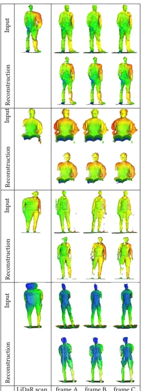
MIG ’18, November 8–10, 2018, Limassol, Cyprus B. Fulop-Balogh et al. Input Re construction Input Re construction Input Re construction Input Re construction

LiDaR scan frame A frame B frame C

Figure 6: Undistorting LiDaR scans (top rows, left) from con-sumer depth camera sequences (top rows, right). Our re-sult (bottom rows) show higher spatial accuracy than the consumer depth camera while respecting the global motion. Video results can be seen in supplemental materials.

(set here to 150◦). Furthermore the device itself rotates around the vertical axis. A full scan at this resolution takes around 14s. To prevent large static objects giving too much weight to the spatial registration compared to temporal variables, we cropped out the walls and ground of the HR scan.

Figure 6 shows the results of our method applied on several real datasets. By comparing the reconstructed frames to the LiDaR scan, one can see the high frequency details transferred across the frames. The accuracy of the overall motion of our reconstructed sequence can be assessed by observing the corresponding LR frames and the accompanying video.

7.3

Limitations

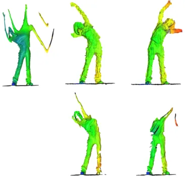
Our method has some limitations. First it can only handle small motions. Large motion over a long time will generate too much distorsion in the LiDAR data and the spacetime registration and point tracking will fail, creating artefacts illustrated in Figure 7. Missing regions can appear due to points being occluded or unob-served in the HR scan during the motion or abnormal time delays between consecutive LR frames causing whole slices of the HR data not corresponding to any LR frame to be lost during the ICP. This produces vertical stripes of missing points in the results (see the last row of figure 6). In this case, merging the LR and HR data would allow for filling in holes.

The depth sensor further suffers from heavy distortions. This is-sue has been identified and investigated by Clarkson et al. [Clarkson et al. 2013] and Herrera et al. [2012], who both propose calibration procedures. As we wanted to remain calibration-free, we did not investigate this issue further. However, our reconstructions are of limited accuracy, exhibiting spatially low-frequency artifacts, that can be attributed to these distortions. Aside from a calibration procedure, our registration process and hence the final reconstruc-tion could be improved by swapping out the ICP algorithm for a non-rigid registration step. We hope even better results could be achieved in the future using this approach.

8

CONCLUSION

We introduced a way to capture animated scenes and produce high resolution point sets by combining a consumer depth sensor and a high precision Time-of-Flight scanner. We showed that by formulating the problem in spacetime we were able to register the datasets and advect details across the frames to undistort moderate motion sequences.

Acknowledgments. This work was funded by Agence Nationale de la Recherche, ANR PAPS project (ANR-14-CE27-0003).

REFERENCES

C. Ancuti, C. O. Ancuti, and P. Bekaert. 2010. Video super-resolution using high quality photographs. In 2010 IEEE International Conference on Acoustics, Speech and Signal Processing. 862–865.

Dana H Ballard. 1981. Generalizing the Hough transform to detect arbitrary shapes. Pattern recognition 13, 2 (1981), 111–122.

S. Berkiten, M. Halber, J. Solomon, C. Ma, H. Li, and S. Rusinkiewicz. 2017. Learn-ing Detail Transfer based on Geometric Features. In Computer Graphics Forum, Proceedings Eurographics 2017.

P. J. Besl and N. D. McKay. 1992. A method for registration of 3-D shapes. IEEE Transactions on Pattern Analysis and Machine Intelligence 14, 2 (Feb 1992), 239–256. Pravin Bhat, C. Lawrence Zitnick, Noah Snavely, Aseem Agarwala, Maneesh Agrawala,

Figure 7: Failure case: large motion are not handled well by our method. Left: Lidar Scan. Depth sensor frames (top row) and corresponding corrected frames (bottom row).

Enhance Videos of a Static Scene. In Proceedings of the 18th Eurographics Conference on Rendering Techniques (EGSR’07). Eurographics Association, 327–338. Derek Bradley, Wolfgang Heidrich, Tiberiu Popa, and Alla Sheffer. 2010. High

Resolu-tion Passive Facial Performance Capture. ACM Trans. on Graphics (Proc. SIGGRAPH) 29, 3 (2010).

D. Herrera C., J. Kannala, and J. HeikkilÃď. 2012. Joint Depth and Color Camera Calibration with Distortion Correction. IEEE Transactions on Pattern Analysis and Machine Intelligence 34, 10 (Oct 2012), 2058–2064. https://doi.org/10.1109/TPAMI. 2012.125

Yaron Caspi and Michal Irani. 2002. Spatio-Temporal Alignment of Sequences. IEEE Trans. Pattern Anal. Mach. Intell. 24, 11 (Nov. 2002), 1409–1424.

Sean Clarkson, Jonathan Wheat, Ben Heller, J Webster, and Simon Choppin. 2013. Distortion correction of depth data from consumer depth cameras. 3D Body Scanning Technologies, Long Beach, California, Hometrica Consulting (2013), 426–437. James Davis, Diego Nehab, Ravi Ramamoorthi, and Szymon Rusinkiewicz. 2005.

Space-time Stereo: A Unifying Framework for Depth from Triangulation. IEEE Trans. Pattern Anal. Mach. Intell. 27, 2 (Feb. 2005), 296–302.

Richard O Duda and Peter E Hart. 1972. Use of the Hough transformation to detect lines and curves in pictures. Commun. ACM 15, 1 (1972), 11–15.

D. Fleet and Y. Weiss. 2006. Optical Flow Estimation. Springer US, Boston, MA, 237–257. https://doi.org/10.1007/0-387-28831-7_15

Ankit Gupta, Pravin Bhat, Mira Dontcheva, Oliver Deussen, Brian Curless, and Michael Cohen. 2008. Enhancing and Experiencing Spacetime Resolution with Videos and Stills, In International Conference on Computational Photography.

Bjoern Haefner, Yvain QuÃľau, Thomas MÃűllenhoff, and Daniel Cremers. 2018. Fight Ill-Posedness With Ill-Posedness: Single-Shot Variational Depth Super-Resolution From Shading. In The IEEE Conference on Computer Vision and Pattern Recognition (CVPR).

A. Hamdi-Cherif, J. Digne, and Chaine R. 2018. Super-resolution of Point Set Surfaces using Local Similarities. to appear in Computer Graphics Forum 37, 1 (2018), 60–70. E. Herbst, X. Ren, and D. Fox. 2013. RGB-D flow: Dense 3-D motion estimation using color and depth. In 2013 IEEE International Conference on Robotics and Automation. 2276–2282.

F. Huguet and F. Devernay. 2007. A Variational Method for Scene Flow Estimation from Stereo Sequences. In 2007 IEEE 11th International Conference on Computer Vision. 1–7. https://doi.org/10.1109/ICCV.2007.4409000

Yong Joo Kil, Boris Mederos, and Nina Amenta. 2006. Laser Scanner Super-resolution. In Proc. Point-Based Graphics (SPBG’06). 9–16.

T. P. Koninckx and L. Van Gool. 2006. Real-time range acquisition by adaptive struc-tured light. IEEE Transactions on Pattern Analysis and Machine Intelligence 28, 3 (March 2006), 432–445.

D. Liu, J. Gu, Y. Hitomi, M. Gupta, T. Mitsunaga, and S. K. Nayar. 2014. Efficient Space-Time Sampling with Pixel-Wise Coded Exposure for High-Speed Imaging. IEEE Transactions on Pattern Analysis and Machine Intelligence 36, 2 (Feb 2014), 248–260.

Niloy J. Mitra, Simon Flöry, Maks Ovsjanikov, Natasha Gelfand, Leonidas Guibas, and Helmut Pottmann. 2007. Dynamic Geometry Registration. In Proc. Symposium on Geometry Processing (SGP ’07). Eurographics, 173–182.

OpenNI organization. 2017. OpenNI User Guide.

J. Quiroga, T. Brox, F. Devernay, and J. Crowley. 2014. Dense semi-rigid scene flow estimation from RGBD images. In European Conference on Computer Vision (ECCV). http://lmb.informatik.uni-freiburg.de/Publications/2014/Bro14

Damien Rohmer, Tiberiu Popa, Marie-Paule Cani, Stefanie Hahmann, and Alla Sheffer. 2010. Animation Wrinkling: Augmenting Coarse Cloth Simulations with Realistic-looking Wrinkles. In ACM SIGGRAPH Asia 2010 Papers. ACM, New York, NY, USA, Article 157, 8 pages.

E. Shechtman, Y. Caspi, and M. Irani. 2005. Space-time super-resolution. IEEE Transac-tions on Pattern Analysis and Machine Intelligence 27, 4 (April 2005), 531–545. Thibaut Weise, Sofien Bouaziz, Hao Li, and Mark Pauly. 2011. Realtime

Performance-based Facial Animation. ACM Trans. Graph. 30, 4, Article 77 (July 2011), 10 pages. T. Weise, B. Leibe, and L. Van Gool. 2007. Fast 3D Scanning with Automatic Motion Compensation. In 2007 IEEE Conference on Computer Vision and Pattern Recognition. 1–8.

Li Zhang, Brian Curless, and Steven M. Seitz. 2003. Spacetime Stereo: Shape Recovery for Dynamic Scenes. In IEEE Computer Society Conference on Computer Vision and Pattern Recognition. 367–374.

Li Zhang, Noah Snavely, Brian Curless, and Steven M. Seitz. 2004. Spacetime Faces: High Resolution Capture for Modeling and Animation. ACM Trans. Graph. 23, 3 (Aug. 2004), 548–558.

Song Zhang. 2010. Recent progresses on real-time 3D shape measurement using digital fringe projection techniques. Optics and Lasers in Engineering 48, 2 (2010), 149 – 158. Fringe Projection Techniques.