Boundary-Integral Formulations for Three-Dimensional Fluid-Structure Interaction
by
Van Chi Luu
B.S. Aerospace Engineering, Iowa State University
(1988)
Submitted to the
Department of Aeronautics and Astronautics
in Partial Fulfillment of the Requirements for the Degree of Master of Science
at the
MASSACHUSETTS INSTITUTE OF TECHNOLOGY
September 1991 @ Van Chi Luu, 1991
The author hereby grants MIT permission to reproduce and to distribute copies of this thesis document in whole or in part.
Signature of Author
Department of Aeronautcic'nd Astronautics August 1, 1991
Certified by,
(j.r. David S. Kang
Thesis Advisor Charles Stark Draper Laboratory Certified by
Accepted by
Professor John Dugundji Thesis Supervisor Department of Aeronautics. axd Astronautics
r-Poi-fes-r Harold Y. Wachma,
Chairman, Department Graduate Committee
--- ---~
----Boundary-Integral Formulations for
Three-Dimensional
Fluid-Structure Interaction
by
Van Chi Luu
Submitted to the Department of Aeronautics and Astronautics on August 1, 1991 in Partial Fulfillment
of the Requirements for the Degree of Master of Science
at the
MASSACHUSETTS INSTITUTE OF TECHNOLOGY
ABSTRACT
Numerical techniques are presented for the determination of the added mass matrix and the excess pressure induced in a fluid of infinite extent by a totally submerged vibrating elastic structure. For relatively low vibrational frequencies, the effect of the surrounding fluid can be incorporated into an added mass matrix merely superimposed upon the structural mass matrix for the solution of the structural response. For higher vibrational frequencies, the simultaneous solution of the elastic and fluid field relationships is required in order to solve the general interaction problem. For this coupled fluid-structure interaction problem, the elastic response of the structure is modeled using finite element method. The acoustic field equations relating the structure's surface pressure and its surface normal velocities are used to form an acoustic impedance matrix, which gives an expression for the fluid-structure interaction forces. These forces are then coupled with the external applied forces, the structural mass matrix, and the stiffness matrix to form the dynamic equilibrium equations for the coupled system.
Thesis Advisor: Dr. David S. Kang
Acknowledgements
I would like to express my sincere gratitude to my thesis advisor, Dr. David S. Kang, for his countless guidance and encouragement. Unlike many professors/researchers in many universities, Dr. Kang cares not only about the education of his students, he also pays great attention to their welfare. Being a master student at M.I.T. for the last two years was exciting and challenging. However, the inevitable stress and frustration that come with being a graduate student would have driven me to insanity without the continuous moral support and helps of Dr. Kang. I owed my education to Dr. Kang, and I appreciate very much for everything he has done for me.
I would like to thank all my colleagues at the Draper Laboratory for their friendship and support: Naz Bedrossian,
Howard Clark, Joe Nadeau, Ashok Patel, and Dave Roberts.
Special thanks go to Naz Bedrossian and his wife for all their helps in the last two years.
Last, but not least, I would like to thank my family and all my friends in Iowa and St. Louis, especially my friends at McDonnell Douglas Missile Systems Company.
This research was done at The Charles Stark Draper Laboratory, Inc.
Publication of this report does not constitute approval by the Charles Stark Draper Laboratory, Inc. of the findings or conclusions contained herein. It is published for the exchange and
stimulation of ideas.
I hereby assign my copyright of this thesis to The Charles Stark Draper Laboratory, Inc., Cambridge, Massachusetts.
Van Chi Luu
Permission is hereby granted by The Charles Stark Draper Laboratory, Inc. to the Massachusetts Institute of Technology to reproduce any or all of this thesis.
Table of Contents
A b stra ct ... 2
A cknow ledgem ents ... ... ... 3
Table of Contents ... 4
List of Figures ... 6
Section 0 . Introduction... 8
1. Low Frequency Fluid-Structure Interaction... 10
1.1 Added Mass Calculation Using Boundary Integral M ethod... ... 11
1.2 Calculation of the Potential and Velocity Induced by a Quadrilateral Element at a Point in Space... ... 20
1.3 Numerical Examples ... ... 7
Case 1 Square Plate with Free-Free Boundary Conditions ... ... 3 9 Case 2 Square Plate with Simply-Supported Boundary Conditions ... 3
2. Coupling Fluid-Structure Interaction...6 1 2.1 Dynamic Equations for the Structure...62...6 2 2.2 Governing Equations for the External Fluid...67
2.3 The Coupled Fluid-Structure Equations...7 3
2.4 Frequency Limitations ... 7 8
Radiation From a Uniformly Driven Shell Spherical ... 7 9 3. Discussion ... 96 4. Conclusions ... ... 99 References ... 101 Appendix ... 104
A-1 The Helmholtz Equation (Reduced Wave Equation)... 105
A-2 Green's Identities ... 107
A-3 Free-space Green's Function for Laplace's Equation ... 113
A-4 Free-space Green's Function for the Helmholtz Equation ... 114
List of Figures
Figure 1.1 An elastic body immersed in an infinite, inviscid, incompressible fluid... ... 12 Figure 1.2 The receiver point approaches the surface S
along the unit normal from the positive side
of the surface ... 14 Figure 1.3 Discretization of the surface ... 16
Figure 1.4 Local element coordinate system... 21 Figure 1.5 A typical four-noded quadrilateral element
and its local coordinates ... 22 Figure 1.6 Local cylindrical coordinate system (looking
down from the positive ý axis) ... 23... 3 Figure 1.7 Contribution of each side of the element to
the potential ... ... ... 2 5 Figure 1.8 a) The point (x, y, 0) lies outside of the element.
b) The point (x, y, 0) lies inside of the element...26 Figure 1.9 Integration over a side of the element...2 28 Figure 1.10 Location of the point (x, y, z) from the origin... 32 Figure 1.11 FFFF boundary conditions-first mode frequency
convergence history (no added mass)...40....4 Figure 1.12 FFFF boundary conditions-first mode frequency
absolute error ... ... 4 1 Figure 1.13 FFFF boundary conditions-first mode frequency
convergence history (with added mass) ... 43...4 3 Figure 1.14 FFFF boundary conditions-first mode frequency
absolute error (with added mass)...44 Figure 1.15 FFFF boundary conditions-modes 1-4
fnum/fexact (with added mass)... ... 4 6
Figure 1.16 FFFF boundary conditions-modes 1-4
natural frequency percent error (with added
m ass)... ... 4 7 Figure 1.17 FFFF boundary conditions-modes 1-4
natural frequencies ... ... 8 Figure 1.18 FFFF boundary conditions-first mode natural
frequency with and without added mass ... 50...5 0 Figure 1.19 FFFF boundary conditions-modes 1-4 natural
frequencies (without added mass) ... 5 1 Figure 1.20 FFFF boundary conditions-modes 1-4 natural
Figure 1.21 SSSS boundary conditions-modes 1-4 natural
frequencies (no added mass) ... 55 Figure 1.22 SSSS boundary conditions-modes 1-4
fnum/fexact (no added mass)... 5 6
Figure 1.23 SSSS boundary conditions-modes 1-4
percent error (no added mass)...5 7 Figure 1.24 SSSS boundary conditions-modes 1-4 natural
frequency convergence histories (with added
mass)... ... 5 8
Figure 1.25 SSSS boundary conditions-modes 1-4
fnum/fexact (with added mass) ... . 5 9
Figure 1.26 SSSS boundary conditions-modes 1-4 natural
frequencies ... ... 6 0 Figure 2.1 An elastic body immersed in an infinite, inviscid,
incompressible fluid... ... 6 8 Figure 2.2 Surface pressure convergence history, Ka = 1.0...8 3 Figure 2.3 Surface pressure convergence history, Ka = 2.0... 84 Figure 2.4 Surface pressure convergence history, Ka = 3.0... 85 Figure 2.5 Surface pressure convergence history, Ka = 4.0... 86 Figure 2.6 Surface pressure absolute error, Ka = 1.0... 8 7 Figure 2.7 Surface pressure absolute error, Ka = 2.0...8 8 Figure 2.8 Surface pressure absolute error, Ka = 3.0...8 9 Figure 2.9 Surface pressure absolute error, Ka = 4.0...90....9 Figure 2.10 Percent error, Ka = 1-4 ... 9 1 Figure 2.11 Maximum percent error, Ka = 1-4 (243
surface elem ents) ... ... 9 2 Figure 2.12 Surface pressure as function of Ka ... 9 3 Figure 2.13 Far-field pressure, r = 2.0 m, Ka = 1.0 ... 94...9 4 Figure 2.14 Far-field pressure, r = 2.0 m, Ka = 3.0 ... 9 5
0. Introduction
Structural vibrations in a fluid are usually coupled to motion of the surrounding fluid. The natural vibrational frequencies, the mode shapes of the structure, and the far-field acoustic pressure induced by the vibrating structure must be found, in general, from a coupled fluid-structure analysis. If the structure is immersed in a fluid of which the density is much less than the average density of the structure (say, for example, air), the effect of the surrounding fluid on the natural frequencies and mode shapes of the structure can be neglected. On the other hand, if the density of the fluid is of the same order of magnitude as the average density of the structure (such as water), the surrounding fluid can alter the natural frequencies and mode shapes of the structure significantly; thus, the presence of the fluid cannot be neglected and a coupled fluid-structure problem must be solved in order to obtain the correct natural frequencies and mode shapes.
At low vibrational frequencies, however, it is known that the fluid pressure on the wetted surface of the structure is in phase with the structural acceleration, and the surrounding fluid appears to the structure like an added mass. Thus, for relatively low frequencies1 the effect of the fluid on the structure are embodied in an added mass matrix that is merely superimposed upon the structural mass matrix. At higher frequencies, the fluid impedance (the ratio of fluid pressure to velocity) is mathematically complex, since both mass-like and damping-like effects are involved. In this case, the fluid can no longer be treated simply as an added mass to the structure and the external fluid equations must be coupled to the structural equations in order to obtain solutions to the interaction problem.
L 2 2
1 Low frequency implies that X << X, where 'st is a characteristic structure wave length for the motion of the structure's surface, and
Xac = c/f is a characteristic acoustic wave length for the motion where f is a characteristic frequency and c is the speed of sound in that fluid. Therefore, if the applied excitation frequencies are less than roughly one-third of the structure's lowest natural frequency of vibration, the effect of the fluid can be incorporated into an added mass matrix superimposing on the structural mass matrix.
The main goal of this thesis is to address the steady state fluid-structure interaction problem described by a totally submerged vibrating elastic body in an acoustic medium of infinite extent. Both low and high vibrational frequencies of the structure will be studied using boundary integral equation (BIE) method. Boundary integral equation formulations are chosen because they appear to be more attractive for this problem as compared to other popular numerical techniques such as finite element or finite difference,2 since they 1) reduce the
dimensionality of the problem by one, 2) obviate the need to model the infinite far-field boundary condition of the acoustic medium, 3) are flexible in handling arbitrary boundary conditions,
and 4) can easily handle arbitrary geometries.
The main structure of this thesis can be divided into two parts: 1) to calculate the added mass matrix for low frequency vibrations of a totally submerged structure, and 2) to calculate the surface and the far-field pressures of a totally submerged vibrating body using the integral Helmholtz equations.
2 Currently, this is the general feeling among researchers in the acoustic field. However, advances in other field in recent years may change this in the future. See the discussions in Section 3.
1. Low Frequency Fluid-Structure Interaction
For fluid-structure interaction situations where the fluid viscosity effects are negligible and the vibrational frequencies are low, the fluid can be treated as inviscid and incompressible (Refs.
16, 17). The added mass calculation then requires solving
Laplace's equation in the fluid domain exterior to the structure. This calculation can be performed using either boundary integral method or finite element method, among others. Sections 1.1 and 1.2 describe in details the theoretical basis and numerical procedure for calculating the added mass matrix using the boundary integral method.
1.1
Added Mass Calculation Using Boundary
MethodConsider a three-dimensional elastic body immersed and at rest in an infinite, inviscid, incompressible fluid which is also at rest. If the surface of the body is made to oscillate about its equilibrium position, the resulting motion of the fluid will be irrotational and acyclic (Ref. 17); hence, the velocity can be expressed as the negative gradient of a scalar potential function (P, that is, V = -Vp. Also, in such a motion the pressure exerted by the fluid on the surface of the body is finite, and to generate the motion the body requires only a finite amount of energy, which is shared between the fluid and the body. The kinetic energy of the fluid is therefore finite, and so the velocity of the fluid at infinity must be zero. Thus, the governing equation for the fluid motion is Laplace's equation
V
2p = 0, (1.1a)and the boundary conditions are
VPn - g' = -lul (1.lb)
on the surface and
IVp I = 0 (1.1c)
at infinity. The vector n in Eq. (1.1b) is the outward unit normal at the surface, Iuis the surface velocity in the normal direction [both
a and a are defined as positive pointing into the fluid (Fig. 1.1)],
and V is the gradient operator. The problem defined by Eqs. (1.1a-c) is known as the external Neumann problem. According to Sobolev (Ref. 21), the solution of an external Neumann problem which has continuous first-order derivatives right up to the boundary is unique, and the solution of the problem can be determined to within an arbitrary additive constant. Many methods, both analytic and numerical, have been developed for solving this problem. One of the classical methods is to reduce the problem to an integral equation over the boundary surface.
... ... ... ... ...
...~~~:
r·. :... . ... . . ...-.
::::.::~iii~il:·lil iI ::.... ~ i~ii::i~i:... ... ...
iiiiii:~~~!~: iiri:~tili: :ii:ii ~ :iii ~liiriii~liiiicii~iiZ~i ... .... .........
Figure 1.1 An elastic body immersed in an infinite, inviscid, incompressible fluid.
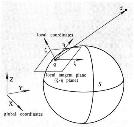
Consider a unit point source located at a point q on the surface of the body whose Cartesian coordinates are Xq, Yq, zq. At
another point d in the fluid domain (with coordinates x, y, z) the potential induced at this point by the point source at q is3
p (d) = 1 (1.2)
Ir(d, q)l
where Ir(d, q)l is the distance between the points d and q (Fig. 1.1), namely,
3 Except for a factor of 1/4n, this is known as free-space Green's function for Laplace's equation. r(d, q) means the distance between points d and q where d represents a point ranging throughout the fluid domain D and q represents a point ranging only over the boundary S.
Ir_(d, q)l -= [(x - X,)2 + (y - yq)2 + ( - zq)2] . (1.3) In this equation q is usually referred to as the "source point" and d the "receiver point." The potential in Eq. (1.2) is a singular solution to Laplace's equation. It satisfies Eq. (1.1a) and Eq. (1.1c) at all points except the source point q. Because of the linearity of Laplace's equation, the potential due to any ensemble or continuous distribution of such sources that lies entirely on the boundary surface S (or interior to S) will also satisfy Eq. (1.1a) and Eq. (1.1c) in D exterior to the boundary. Therefore, a solution
based on a continuous source distribution on the surface S can be formulated. If the source density (source per unit area) at a given point on the surface is denoted by 0(q), then the potential at the receiver point d due to the continuous distribution of source at the surface is4
p (d)
([
d)S.
(1.4)
[ r_(d, q)I
Eq. (1.4) expresses the velocity potential (P at an arbitrary point d in terms of an integral over the boundary of the fluid domain D.
Regardless of the nature of the source density function 0(q), the potential given by Eq. (1.4) satisfies two of the three equations of the external Neumann problem. The surface source density function is determined from the requirement that the potential must also satisfy the Neumann boundary condition, namely, Eq. (1.1b). Applying the boundary condition (1.1b) requires the evaluation of the limits of the spatial derivatives of Eq. (1.4) as d approaches a point s on the surface S (Fig. 1.2). Care is required in taking the derivatives of Eq. (1.4) because the derivatives of the integrand 1/1r(d, q)l become singular as the surface is approached. When Eq. (1.4) is differentiated and the Neumann boundary condition is applied to it by allowing point d to approach point s, the result is the following expression for the surface source
density distribution function 0(q):
4 dS = dS(q) indicating that it is a surface element at point q: when q shifts,
a9p o(q) cos [0(s, q)]
Vp - -2 7 (s)+ ()COSo((s q)]+ dS (1.5)
fn+s Irf(s, q)12
D (fluid .domain)
S( d,iq)
Figure 1.2 The receiver point approaches the surface S along the unit normal from the positive side of the surface.
where O(s, q) is the angle between the unit normal at the source
point and the vector r(s, q), and aq' / an+ is the normal derivative of (P on the boundary S approaching from the positive side of the surface. Eq. (1.5) is known as a Fredholm integral equation of the
second kind. The term 2 n o(s) arises from the delta function that
is brought in by the limiting process of approaching the boundary. It represents the contribution to the outward normal velocity at point s from the source density in the immediate neighborhood of
s. The surface integral represents the contribution to the normal
... .... ..
velocity at s from the source density of the remainder of the boundary surface (Ref. 15).
Closed-form analytic solutions to Eqs. (1.4) and (1.5) are rare except for simple geometries. For arbitrary three-dimensional bodies, these integrals must be solved numerically. This can be accomplished in the following manner. The surface of the body is approximated by quadrilateral elements whose characteristic dimensions are small compared to those of the body. Over each element the value of the surface source density is assumed constant. This approximation reduces the problem of determining a continuous source density function a(q) to that of determining a discrete number of value of ai, one for each surface element. After the above procedure is completed, the unknown source distributions are eliminated from the equations. The fluid mass matrix is determined from a variational principle based on the fluid kinetic energy expression
KEf :- f f ((p'(m) <p(m)) dS, (1.6) where KEf and Pf are the kinetic energy and the density of the
fluid, respectively. The details of the above procedure are as follows. First, the surface of the body is divided into N quadrilateral elements to identify N distinct boundary integral relations (Fig. 1.3). Eq. (1.6) can be written in matrix form as
KEfds = - pf pT dS p (1.7a)
or
KEfydis = Pf j(PdS(p' (1.7b)
where the dimension of the column vectors (P and (P is (N x 1), the
dimension of the diagonal area matrix dS is (N x N), and the
superscript T denotes transpose of a vector or matrix. Next assume that the surface density function can be suitably represented, piecewise over N discrete patches of Sn, by constant on (n = 1, 2, . . ., N). Based on the above assumptions Eqs. (1.4, 1.5) can be rewritten as
=P B (1.8a) C, = -Q (1.8b) . .. ... ... . .. . ... .... . .. .. .. ... .... ... ... . .. .. . . . ... ... ... . .. ... ... ... ... ... ... ... ... ... ... ... .......... ... .. ... .. . . ... .... ... . .. . . . ... .... . .. ... ... .... .. .. . . . .... . ... ... .. . . . ... . ... . .. .. .... ... .. ... .... .... .... ..... ...... ... . . . . .. . . .. . ... ... .. . .... . ..... ... . .... ... .. .. ... .... . . .. . . . . ... .. ... .. .. .... .... ... ... ...... .... . . . . .. . . .. . .
...iiiii . ..:!ii:i~ i~iiiii !::iiiii~ . .. .... .i~ ii~ ~i:!ii ~i~i:i i~.•iiiiiiiiiiii•i~iiiii~ii~iiiii~iiii~iiiiiiiiiii~iiii~ ... ... ... ..... ......~iiiiiiiii~ii...iiiiiiiii ...... . . .. . . .. .iiii~iiii~ ~ii~ ~iii
...: • . ... . . ... :: .: • ..: :: ....: .. ...= .- .... :. ..: ..: .• ..: . .: :: ::::: ... :::::: ... .. .. .. .... : . .• ... : : .. : .. : :. :: ... ::: .. :::: :. .• : :: : :::::::: .• .. .. •. .... ... : :: .... .. :: ..:• : :::: .... : :: :: : ... :: :::::.: .. .. : .... :::.. :: :.: .... :: : .. ..:: .
Figure 1.3 Discretization of the surface.
and the dimension of the matrices B and C is (N x N). Since the 1t
h
component of the source density vector _ is independent of the control point within the ith element (because constant source density within each element was assumed), Eqs. (1.8 a, b) may be expressed in terms of any desired set of control points P. (= [P1, P2,
..., PN]T). Therefore, the potential and the source density vectors may be solved in terms of the surface normal velocity vector
_p(P) = B(P) _(P) (1.9a) (P) = -[C(P)] -' '(P) = [C(P)]- u(P). (1.9b)
I
...... ...... ...... ......... .............................. .................. ... ...... ...... ...... ... ...... ... ... ......... ...In the above equations _(P) (= [(PP1, (P2, . . ., ]T) denotes a set of
discrete value of potentials evaluated at the control points P, g(P) is the control point source density vector, [C(P)]1 is the inverse of the matrix C, and u_(P) is the normal velocity vector at P. Substituting Eqs. (1.8a, b) [with _o = (P)] and Eqs. (1.9a, b) into Eq. (1.7a): -1 .pffs (Td S (p = - p f 2 s -- 2 _ fs -1 T[(P)] ' MP)}
2
P)
IPf
Pr {[.(P)]T LC(p)] T CT) dS {B [C(P)] 1 u(P))2
fS
I= p [(P)]T E [(P)] 2 (1.10) where E= [C(P)' I]T (1.11)Similarly, substituting the same set of equations into (1.7b) yields
--- _l (P)}T 'S-C •(P)} S 1 {. [ (P)]C (P) - 1 TB [C(P) - [- B _1P)} dS [C [C(P)]- uP) } - pf f {[u(P)]T [C(p)-]T BT dS {C [C(P)]" P) } {-C o(P)}r dS {B o_(P)} 1 pf [p) T [C(P)-1 T 2
,ICTddS
B
[C(P)]' u(P)
-fs
[C] OS
B
,1
i C(P
[C(p)-']T = [u(p)lT 2
[!((p)I]
Tj
[(ý(P ) -I]
T
-[S
B
TdSC]
BT dST C
([CT] dS B [C (P) 1 = }T] [C(P)] "1that dST
= dS
since it is a diagonal matrix), can be rewritten as 1 Pf [p )] ]T E [(P)]. 2 Averaging Eq. fluid kinetic e (1.10) and Eq. (1.13) nergy can be expressed asthe discretized version of the
(1.14)
KEf,. = T Mf u 2
where Mf is the fluid mass matrix,
(1.15)
and E is given by the expression in Eq. (1.11). Since constant source density on each element was assumed, the entries of the matrices CT and B in the integral of Eq. (1.11) are constants. Therefore, the integral can be approximated by
[eT ] dS B = [C()] T A [IB(P)] (1.16) Since [C (P)] u(P). (1.12) (note (1.12)
=
ET
therefore, Eq. (1.13) Mf = 1 pf [E + ET], 2where A is the (N x N) diagonal matrix (aii is the area of the ith surface element). Substituting Eq. (1.16) for the integral in Eq. (1.11) yields
E [(p)-I]TL [T] dS B] [C(P)]1
= [C(p)] T [C(P)]T A [B(P)] [((P)]-1 or
E = A [B(P)] [C(P)]' . (1.17)
From Eqs. (1.15) and (1.17), it is seen that the calculations of the matrices B(P) and C(P) form the basis of the present method for the added mass calculation. The entries of the matrices B(P) and C(P) are the potentials and velocities, respectively, that are induced at the control point of the ith element by a unit point
source density on the jth element. They are obtained by integrating over the element in question the formulas for the potential and velocity, namely, Eqs. (1.4) and (1.5). With unit source density Eqs. (1.4) and (1.5) depend only on the location of the point at which the potential and velocity are being evaluated and the geometries of the source elements; therefore, for simple quadrilateral elements the integration of Eqs. (1.4) and (1.5) over the source elements can be performed analytically.
1.2 Calculation of the Potential and Velocity Induced by a Quadrilateral Element at a Point in Space
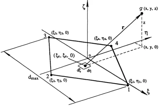
From the discussion in the last section, it is clear that the added mass matrix can be assembled once the potential and velocity matrices are obtained. The purpose of this section is to derive the formulas necessary for calculating the entries of matrices B(P) and C(P). Following the procedure outlined in Ref. 12, the formulas are obtained by performing the integration of the basic point-source equations over a surface element. For quadrilateral elements used to approximate the surfaces of three-dimensional bodies, the integration of Eq. (1.4) is most conveniently done in local element coordinate system. Consider a typical surface element as shown in Fig. 1.4. A local coordinate system (, 11, C) is chosen such that the origin of the coordinates is located at the centroid of the element. The element is taken to lie in the r1l-plane, and the ý-axis points in the direction of the unit outward normal of the element. Assuming that four-noded quadrilateral elements are used to approximate the surface of the body. The four corner points of the element are denoted by subscripts 1-4, where the numbering denotes the order in which the corner points of the element are encountered as one traverses along the perimeter in a clockwise sense (as view from the positive p-axis). In the ýr1-plane the coordinates of the corner
points are ýn, rln, 0 where n = 1-4. The maximum dimension of the
element is denoted by dmax (Fig. 1.5). In order to facilitate the calculations of certain equations to be derived later, the a-axis is taken to be parallel to the vector from corner point 1 to corner point 3. Consider a point g in space with local coordinates x, y, z
(Fig. 1.5). The distance between this point and a point (e, Tle, 0) on
the element in question is
, Z
Y
x
c r
global coordii
Figure 1.4 Local element coordinate system.
For a unit point source density, the potential at the point (x, y, z) induced by an infinitesimal element d( drl is
drp = 1 dý dr 1= dA .
(1.19)
T13, 0)
Sz)
0)
Figure 1.5 A typical four-noded quadrilateral element and its local coordinates.
The total potential at (x, y, z) induced by the quadrilateral element is then
p(x, y,z) =
fdp
=
f
] dA,
(1.20)
where the domain of the area integral is the surface element. In order to facilitate the integration of Eq. (1.20), a cylindrical coordinate system, (R, 0, z), with origin situated at the point (x, y, 0) is introduced (Fig. 1.6). In this coordinate system, A is the radial distance from (x, y, 0) to a point on the element, 0 is the polar angle measured clockwise from any convenient reference axis, and z is taken to be parallel to the C-axis. In terms of these new variables Eq. (1.18) can be written as
(53~ Ti3, )
(~4, 114, 0)
y,
0)
Figure 1.6 Local cylindrical coordinate system (looking down from the positive C axis).
Substituting Eq. (1.21) into Eq. (1.20) the potential at (x, y, z) induced by the element becomes
<p(x, y, z) = i dA= 1 + z d A
sJ
A ji
#2
+z
2
1
= - dR dOS
2+ z2
dRd
(1.22)
or p(x, y, z) = R d dO. (1.23)Jof
J0
2
+ z
2
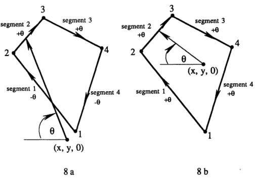
~t aIn Eq. (1.23) the integration limits of the A variable is from A = 0 to a point on the perimeter of the element A = R , and the integration limits of the 0 variable is around the perimeter of the element from 0 to 2 t in a clockwise sense (Fig. 1.6). The contribution of each side of the element to Eq. (1.23) represents the potential of the plane triangle defined by the point (x, y, 0) and the two end points of the line segment (Fig. 1.7). From Fig. 1.7a it is seen that as the perimeter of the element is being traversed in a clockwise sense, d 0 is positive if the point (x, y, 0) is to the right of the line segment (segments 2 and 3) and is negative when the point is to the left of the element (segments 1 and 4). Therefore, when the potential of the four triangles corresponding to all four sides of the element are summed, the contributions of the portions of the triangles outside the element summed to zero (the shaded portion in Fig. 1.7b), and the result would be the contribution of the element itself. From Eq. (1.21) the distance from a point on the element to the point (x, y, z) is
r = 2 ++z 2 (1.24)
Differentiating the above equation yields
dr = A dA (1.25)
i2p
-Substituting Eq. (1.25) into Eq. (1.23) and changing the integration Substituting Eq. (1.25) into Eq. (1.23) and changing the integration limits of the R variable the potential at (x, y, z) becomes
2 n r
Px, y, Z) =i
dr] dO Izl = [r] dO - ij Izlf dO, (1.26) or <p(x, y, z) =f
[r] dO - 8ij Izl A (1.27)AO = d O.
gative
(1.28)
7a 7b
Contribution of each side of the potential. where Figure element 1.7 to the
3 se segm 2 4 4 nent 4 (x, y, 0) 8a 8b
Figure 1.8 a) The point (x, y, 0) lies outside of the element. b) The point (x, y, 0) lies inside of the element.
From Fig. 1.8 it is seen that when the point (x, y, 0) is outside the element AO = 0 (A0's of segments 2 and 3 cancel out AO's of segments 1 and 4), and Ae =2 x if the point (x, y, 0) lies inside the element. (Note that when (x, y, 0) is inside the element the perimeter is always on the right-hand side of (x, y, 0) as it is being traversed, therefore, dO is always positive.) Hence,
<p(x, y, z) = [r] dO (1.29)
if (x, y, z) lies outside of the element and
<p(x,
y, z) = [r] dO - 2 x IzI (1.30)3
vif (x, y, z) lies inside of the element. Thus, the second term of Eq. (1.27) is discontinuous as the point (x, y, 0) crosses a side of the element. However, the first term of the equation has an equal but opposite discontinuity (due to the change of sign of dO along the side that is crossed) and thus the potential is continuous across the surface as expected. The integral of Eq. (1.27) is evaluated by calculating the contribution of a single side to the integral and summing the results for all four sides. (Note that the results can be generalized to polygons having any number of sides.) For the purpose of deriving the equations, the contribution of the side
between the points (1,7 11, 0) and (42,112, 0) is used to illustrate
the procedure. The contributions of the other sides can be found by advancing all the subscripts and superscripts in the equations.
Consider the line segment between (i1, 11, 0) and (42, 12, 0)
as shown in Fig. 1.9 and defining the following geometric
quantities. The length of the side between (1, 7T1, 0) and (42, T12, 0)
is
d12 = V(2- 1)2 + (112 11)2 (1.31) The cosine and sine of the angle 012 are, respectively,
cos012 Ax _ (2-1) - C1 2 (1.32)
di 2 d 12
Ay (1 2-1]) 1
sin12 - - 12 1) -1 S12 . (1.33)
d12 d12
A line perpendicular to segment 1-2 is drawn from the point (x, y, 0), and the (signed) distance from the point (x, y, 0) to the extension of segment 1-2 is
R12 = (x - 41) S12 - (y - 11) C12 . (1.34)
Note that the distance is positive if (x, y, 0) lies to the right of the
side with respect to the direction from (41, TI1, 0) to (42, ti2, 0) and
is negative if (x, y, 0) lies to the left. Let L12 be the distance along
(2, 112, 0), as shown in Fig. 1.9. The arc length associated with a general point (ý, 11) on the side is
L12 = (ý - X) C12 + (rY - y) S12.
(1.35)
P(
2, T12, 0) - (•,rI)
(x, y, 0)
Figure 1.9 Integration over a side of the element.
In particular, the arc lengths associated with the corner points
(ýi1, 1, 0) and (t2, 1r2, 0) are, respectively,
£12 = ;1 - X) (12 + (7Tl - y) S1 2 (2) 12 = (2 - X) C12 + (12 - Y) S12 . (1.36) (1.37) and r /r ,,
The distances from the point (x, y, z) to the corner points (41, 1ll, 0) and (2,9 12, 0) are, respectively,
ri = (x - 1)2 + (y- l)2 + z2 (1.38)
and
r2 = (X - 2)2 + (y- 92 2 + Z2 . (1.39)
With the above geometric variables the following two quantities can be defined: (2) Q12 - lnr2 + L 12 = In r2 (1 40) r +L(1) +L rl + r2 - d12 12 (2) (1) tn [ R12 Iz1 (r1L, 12 - r2 L12) J12 tan [R12 2 2Z 12)] ( (1.41) r1 r2 (R12) 2 (2L L (1
where the range of the inverse tangent in Eq. (1.41) is from -x to nt by considering the individual signs of the numerator and denominator of its argument. With the defined quantities, the contribution of the line segment between (ý1, 11, 0) and (2, 1T2, 0) to the integral in Eq. (1.27) is then
(P12 = R12 Q12 + IzI J12. (1.42) The contributions of other segments of the element are found by advancing the subscripts and superscripts in the above equations. The potential at the point (x, y, z), and also the entries of the B matrix bij, induced by the element is then
bij = p (x, y, z) = [P12 + 9P23 + (34 + (P41] -zI AO (1.43) where (P12, (P23, (P34, and 'P41 are the contributions of the four segments to the integral in Eq. (1.27). The velocity components in
local element coordinates can be found by differentiating the velocity potential: Vx - -a S12 Q12 + S2 3 Q23 + S34 Q34 + S4 1 Q4 1), (1.44) ax Vy - (C 12 Q12 + C23 Q23 + C34 Q34 + C4 1 Q4 1 , (1.45) ay and Vz - - sgn(z) (AO -J12 - J23 -J34 - J41 (1.46) az
where "sgn" is the FORTRAN sign function. The normal velocity at
(x, y, z), and also the entries of the C matrix cij, can be found by
taking the dot product of the velocity vector,
V = Vx i + Vy j + Vz ki, and the unit normal vector at the point (x,
y, z). Thus,
Cij = i ij = (ni i + i2 jni3 k) (Vx i + Vy j + Vz k) or
cij = nil Vx + ni2 Vy + ni3 Vz. (1.47) It can be verified that the above equations encounter no difficulty in calculating the effects of an element at its own control point. All the Q's are singular only on the sides of the element. For z = 0, all the J's vanish. Thus P, Vx, and Vy are regular functions, and for z = 0
Vz = sgn(z) AO, (1.48)
Which is 2 n sgn(z) for a point on the element and zero for a point outside the element. From the discussion in Section 1.1 the control point was defined to have z = 0+. Therefore, AO can be evaluated
easily; it is 2 nt if R12, R23, R34, and R4 1 are all positive, and it is
Eqs. (1.40-1.47) are the required equations for calculating the potential and velocity matrices B and C, respectively. The entries of matrices B and C can be calculated using these
equations without any further approximation. However,
evaluation of Eq. (1.43) requires at least four logarithms, four inverse tangents, and four square roots for each element. For three-dimensional arbitrary bodies the computational time required for calculating the velocity and potential matrices can be prohibitively large. The complication comes from the fact that the above formulas take into account of all the details of the shape of the element. Incidentally, if the receiver point (x, y, z) is located sufficiently far away from the source element, the shape of the source element becomes less significant. Thus if a point (x, y, z) is located at a distance ro from the source element, where ro is the distance between the centroid of the source element and the point (x, y, z) (Fig. 1.10), and if the ratio ro/dmax > 2.45 (dmax is the maximum dimension of the element as defined in Fig. 1.5), Eq. (1.20) can be approximate by expanding the integrand about ro in terms of Taylor series expansion (Ref. 12). Since r was defined as
[(x - 2 + (y - r) 2 + 2]11/2, Eq. (1.20) can be rewritten as
p(x, y, z) = [(x - )2+(y )2 +z2-1/ 2 dA (1.49)
From any standard calculus text book the formula of Taylor series expansion for two variables is
f(x, + Ax, yo + Ay) = f(x,, yo) + (Ax - + Ay
)
f(x, y) +ax ay
1 (Ax + Ay )2 (x0, Yo) + + i(---i+Ay• 2! ax )2f(xo, yo)+...+
ay
(Ax + Ay ) n f(xo + m Ax, yo + m Ay)
n! ax ay
(p3, (42, y, z) (1, Trl, O) Figure 1.10 origin.
Location of the point (x, y, z) from the
Applying Eq. (1.50) to the integrand of Eq. (1.49):
+ [ 14 1 +
n
0
ax ro
1)]
+ 1 [ 02 2 y ro 2! 2 ro 2 2 9 a2 1 ) 1 + ax2y ox (1)ro
dA +
=f 2 2 a2 -2 (-)+2 jyx aX2 o ax ay P = 00 w - (llo Wx (1)+ I-ro
ay ro
(L:)] dA+ R a[a
ex 2 ( + 12 (-)] dA+..., (1.52) ro a2 0 o + io0 wy) +1 (120 Wxx + 29
=
(1.51) 1 2! ~r I rl ,I2
2 1 )]+...} dA y2 ko2 111 Wxy + 102 Wyy) + . . ., (1.53) where Imn m 11n dA, (1.54) w ro 1 , (1.55) /(x2 + y2 + z2)
and the subscripts x and y in Eq. (1.53) denote partial derivatives with respect to x and y, respectively. The integral terms Imn are the moments of various orders of the area of the element about the origin. In particular, 10 0 is the area of the element, I1 o and I0 1
are the first moments, and 120, 11 1, and 102 are the second
moments etc. The various terms in Eq. (1.53) may be interpreted as the potentials of point singularities of various orders located at the origin. Thus the first term in Eq. (1.53) is the potential of a point source; the second group of terms is the potentials of two dipoles, whose axes lie along the x-axis and the y-axis, respectively; and the third group of terms is the potentials of the three independent point quadrupoles with axes in the xy-plane. The strengths of the singularities are the various moments of the area of the element. In actual calculation the series is truncated after the quadrupole terms in Eq. (1.53). Since the origin of the coordinate system is located at the centroid of the element, the first moments lho and 0lo are identically zero. Therefore, for centroidal control points there are no dipole terms in Eq. (1.53), only a source term plus the quadrupole terms. Thus, the approximation of Eq. (1.20) may be written as
= I00 w + 1 (120 Wxx + 2 111 wxy + 102 Wyy), (1.56)
2
Vx - 4oo wx 1 (20 Wxxx +
ax 2
V Y - - loowy -- (2o Wxxy+ ay 2 2 111 Wxyy + 102 Wyyy), Vz = -aP = - -o 4w 100 Wz- 1 (120 Wxxz ++
az
2
2 111 Wxyz + 102 Wyyz),where w and its derivatives are
w = ro-1 wx = -x ro-3 Wy = -y ro-3 Wz = -z ro-3 Wxx = -(f + 2 x2) ro -5 wxy =
-(3
xy)
ro-5Wyy = -(f + 2 y2) ro-5
Wxxx = 3 x (3 f + 10 x2) ro-7 wxxy = 3yf ro7 Wxyy = 3 x h ro-7 Wyyy = 3 y (3 h + 10 y2) ro-7 Wxxz =
3zf
ro7 W yyz = -15 x y z ro-7 Wyyz f = y2 + z2 - 4 x2, = 3 zh ro-7 h = x2 + z2 - 4 y2.The moments Imn may be expressed in terms of the coordinates of the corner points of the element [remember that the 4-axis was
taken to be parallel to the vector from (I1, T11, 0) to (3, 113, 0)] as
follows: o00 = - 3 - 1) (12- 114)1 2 120 - (42- 41) 111 (54 - 42) (41 + 42 + 43 + 44) + (12- O4) 12 (1.57b) (1.57c) and (1.58)
2 2 (41 + 41 43 + 42) + 42 T12 (41 + 42 + 3) - 44 114 (41 + 43 + 44)1, 111 1 (43- 1) [244 (412_ .12) 2 ,n2 _n 2) + (41 + 3) 24 (012 - 14) (2 11 + 312 + T14)], and IO2 - (43 - 41) (12 - 14) [(31 + 112 + T14)2 -12 11 1 (12 + T14) - 712 T14] (1.59)
Further approximation to Eq. (1.53) can be made if the ratio
ro/ dmax is greater than 4. For ro/ dmax > 4 the quadrupole terms [all
the terms multiplied by the 1/2 in Eq. (1.53)] are insignificant. Therefore, those terms can be ignored without compromising the accuracy. The quadrilateral element may further be approximated by a point source located at its centroid. For this calculation there is no need to transform to the element coordinate system. The calculation may be performed directly in the global coordinate system. Let xo, Yo, zo be the global coordinates of the centroid of
the element, and let xr, Yr, Zr be the global coordinates of the
receiver point. The potential and velocity components are then
P = 100oo (1.60) ro Vx = Xr-xo l00, (1.61a) Vy = yr - Yo 100, 3 (1.61b)
ro
Vz = Zr- o I00oo, (1.61c) wherewhere
ro = V/[(Xr- Xo)2 + (Yr - o)2 + (Zr Zo)2] .
Note that the above equations are equivalent in accuracy to a source plus a dipole (since the dipole terms = 0 for centroidal control points).
From the above analysis, it is seen that three set of formulas for calculating the potential and velocity induced by a surface element at a point in space can be used. The choice of which set of equations to used is determined solely by the value of the ratio ro/dmax. Ifr o/dmax is less than 2.45 (an arbitrary choice) then the (numerical) exact formulas Eqs. (1.40-1.48) are used; if r/ dmax is greater than 2.45 but is less than 4, the multipole-expansion formulas, Eqs. (1.56-1.59), are used; and if rd dmax is greater than 4 the potential and velocity can be calculated directly in the global coordinate system with Eqs. (1.60-1.61).
1.3
Numerical Examples
Analytical added mass solutions of three-dimensional bodies are scarce owing to the lack of three-dimensional theories. Most of the existing theoretical solutions in the literature are for simple geometries such as rectangular plates, circular plates, and triangular plates etc. In order to be able to compare the numerical solutions with the analytical solutions, a square plate whose physical and material parameters as given in Table 1.1 will be
used for the two examples followed.
Young's modulus E = 6.895(1010) N/m 2 Poisson's ratio v = 3.000(10 1) Density P = 7794.6 Kg/m3 Length L = 3.048(10- 1) m Width W= 3.048(10- 1) m Thickness h = 3.048(10 -3) m
Table 1.1 Material properties for the plate.
The computational scheme presented in Section 1.2 was programmed in FORTRAN for the solution of the added mass matrix with a minimum of six finite element grids for each case. Outputs from the program were then compared to the exact solutions. All the analytical solutions given in this section were obtained from Ref. 3. The equation for the exact natural frequencies of rectangular plates is given by
fij - 2•i E ; i = 1, 2, 3,... (1.62)
2 L2
12 y (1-v2)
j = 1,
2, 3,...
where 7 = mass per unit area of the plate, i = number of half-waves in mode shape along horizontal axis, j = number of half-waves in mode shape along vertical axis, and ?ij is the dimensionless frequency parameter. The dimensionless frequency parameter Xij is generally a function of the boundary conditions applied to the edges of the plate, the aspect ratio of the plate (L/W), and in certain cases Poisson's ratio (v):
kij = kij(boundary conditions, L/W, v).
The natural frequencies of the first six modes of rectangular plates for all 21 possible combinations of the three elementary boundary conditions on the four edges of the plates (clamped, free, simply supported) are given in Ref. 3. The following two cases with two different types of boundary conditions were chosen to demonstrate the solution procedure and the results generated by the program. [Note that number of elements in the following examples denotes the total number of elements for the full plate (without symmetry boundary conditions).]
5 It is shown in Ref. 3 that kij is independent of Poisson's ratio V unless one or more edges of the plate are free.
CASE 1 Square
Plate
with
Free-Free
Boundary
Conditions
All edges of the plate are free to vibrate for this case. The analytical solutions for the first four modes for a plate to vibrate
freely in vacuum are f2 2 = 5.283 Hz, f1 3 = 7.750 Hz, f3 1 = 9.568 Hz,
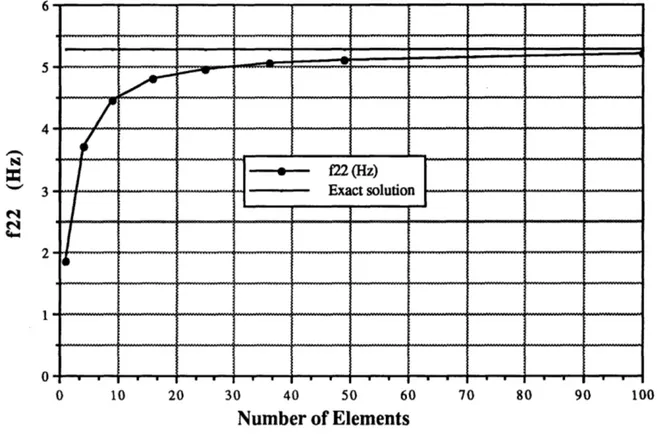
and f32 = 13.715 Hz.6 Fig. 1.11 shows the computed first mode
(f2 2) natural frequency of the plate plotted as function of the
number of elements. The numerical solution is seemed to exhibit rapid monotonic convergence from below. Note that when only one element was used to model the plate, the error is well over
60%. The reason for this large error is due to the fact that lumped
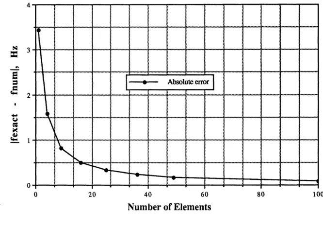
mass formulation was used to calculate the structural mass matrix. For a single quadrilateral element the lumped mass approximation resulted in all the mass of the plate being concentrated in the four corner nodes; hence, the program was not able to capture the first modal vibration in this case. As the number of elements was increased, more elements (and nodes) were being distributed inside the plate and the solution converged rapidly toward the exact solution. Note that for a model of only 36 elements (6 x 6) the numerical solution is already within 2% of the exact solution. Fig. 1.12 presents the absolute error in the computed natural frequency for free vibration of the first mode. The absolute error of the numerical solution starts from 3.429 for a one-element model and decreases to less than 0.09 for a model of 10 x 10 elements.
6 The subscripts are the vibration mode indices. f2 2 is the first nonrigid-body mode for a completely free plate.
0 10 20 30 40 50 60 70 80 90 100
Number of Elements
Figure 1.11 FFFF
frequency convergence
boundary conditions-first mode history (no added mass).
3
2
0
0 20 40 60 80 100
Number of Elements
Figure 1.12 FFFF boundary conditions-first mode frequency absolute error.
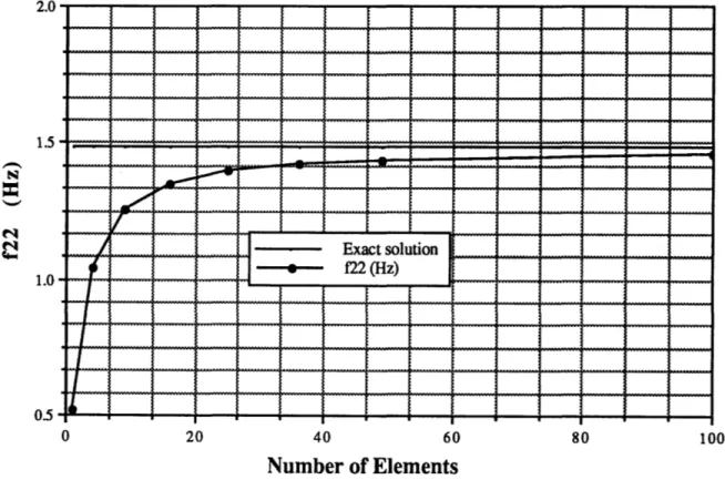
The previous example was valid only for a plate vibrating freely in vacuum. As discussed in the introduction section, the surrounding fluid can alter the natural frequencies of vibration of a structure significantly if the fluid density is of the same order of magnitude as the average density of the structure. If the plate were to vibrate freely in a body of water of infinite extent, the analytical solutions for the first four modes of the natural
frequencies of the plate are f2 2 = 1.485 Hz, f 13 = 2.179 Hz, f31 =
2.690 Hz, and f3 2 = 3.856 Hz. Comparing these frequencies with
the (in vacuum) frequencies given above, one sees that the presence of the water is indeed to have a profound effect on the natural frequencies of the plate. Fig. 1.13 shows the numerical solution of the first mode natural frequency (f2 2) for the plate
vibrating in water. The program based on the scheme presented in Section 1.2 was used to generate the added mass matrix Mf. After the added mass matrix was generated, it was combined with the structural mass matrix as shown in Eq. (1.64) to form the dynamic equilibrium equations for the structure
(Ms + Mf) X + iKs X = F (1.64)
In Eq. (1.64) Ms is the structural mass matrix, K, is the structural
stiffness matrix, and F is the force vector which may include structural damping forces as well as prescribed external forces. From Fig. 1.13, it is seen that the added mass matrix did not seem to affect the convergence rate of the finite element program at all. Note that even with the added mass matrix, the solution still exhibit monotonic convergence. For this case, the computed first mode natural frequency converged to within 1.6% of the analytical solution for a mess of 10 x 10 elements. The absolute error for
this case is presented in Fig. 1.14. Comparing Figs. 1.12 and 1.14, although both plots have the same shape, the absolute error for the case with added mass decreased more rapidly and the absolute magnitude of the error decreased to less than 0.03 for a mesh of 10 x 10 elements.
100
Number of Elements
Figure 1.13 FFFF boundary conditions-first
frequency convergence history (with added mass).
mode
/-..
Exact solution•-~
--
f22 (Hz)
- -- --'-- --' - -- - - -- .. .---.. .. .. .---- - .. .. .. . ... . .. .. .. .. .. .. ... -... -... .. .. .. ---.. .. .. . ... .. .. . ---- ... --...- _• --- --- ---- ---. ---... •... - ---- ---. I -.. -.. -..-- -- --- --.. ... ...- . .. .. .- . .. .. ..- . .. . .- . .. .. .- . .. .. .- .. ..- ..- ---.. -.. ..- -.. --.. -.. . .. .. .---.. -.. ----.. --- -.. . . . .. - - - - . . . . . - - - . . . .. . . . -- - -- - -. . . --- --.. - ---. . . .---..N
Cu
C.
0 20 40 60 80
Number of Elements
Figure 1.14 FFFF boundary conditions-first
frequency absolute error (with added mass).
100
The ratios of numerical to the exact solutions (fnum/fexact) for
the first four modes are presented in Fig. 1.15. Note that only the first mode exhibits complete monotonic convergence. The other three higher modes started from above at the beginning and dropped down rapidly before converging to the exact solutions. For a model of 10 x 10 elements, the first mode converged to within 2% of the exact solution and the other three modes are only within 5%. This information can be seen more clearly in Fig. 1.16. The analytical and the converged numerical solutions (with added mass) for the first four modes of the plate are shown in Fig. 1.17. (The numerical solutions were obtained using a mesh of 10 x 10 elements.) Note that the converged numerical solutions fall almost right on top of the analytical solutions.
1.0 0.5 0.0 0 20 Figure 1.15 fnum/fexact (with a 40 60 80 100 Number of Elements FFFF boundary conditions-modes 1-4 Ided mass).
5
Mode
Figure 1.16 FFFF boundary conditions-modes 1-4 natural
frequency percent error (with added mass). 0
0
%
Error
... --- ...--...-...---...--... ...-...-- ...
0 1 2 3 4 5 Mode
Figure 1.17
frequencies.
Fig. 1.18 compares the first mode natural frequency (f2 2) for
the cases with and without added mass. This figure shows clearly that the inertia of the water cannot be neglected for this case since the water density if of the same order of magnitude as the average structural density. A very large error will result if the inertia effect of the water is neglected when calculating the natural frequencies. Finally, Figs. 1.19 and 1.20 show the first four mode natural frequencies for a freely vibrating plate in vacuum and in water, respectively.
2 0 -1 -2 0.1 0.2 0.3 0.4 0.5 0.6 0 Time, sec.
Figure 1.18 FFFF boundary conditions-first mode natural frequency with and without added mass.
S2 Q 1 -0 N 0-1 -2 0.00 0.10 0.20 0.30 Time, sec.
Figure 1.19 FFFF boundary conditions-modes 1-4 natural frequencies (without added mass).
2 1 0 -1 -2 0.00 0.25 0.50 0.75 1.00 1.25 Time, sec.
Figure 1.20 FFFF boundary conditions-modes 1-4 natural frequencies (with added mass).
CASE 2
Square Plate with Simply-Supported Boundary
Conditions
For this case, all four edges are restrained from moving in all directions but are free to rotate. The (in vacuum) analytical solutions for the first four mode natural frequencies are fl =
7.731 Hz, f2 1 = 19.327 Hz, f1 2 = 19.327 Hz, and f2 2 = 30.923 Hz. Note that the second and third natural frequencies are exactly identical for this set of boundary conditions. The computed first four mode natural frequencies of the plate plotted as function of the number of elements are shown in Fig. 1.21. From the figure, it is seen that all the frequencies started from above at the beginning and dropped below the exact solutions before converging. The convergence histories for the different frequencies are shown in Fig. 1.22. Unlike the previous case, the three higher modes for this set of boundary conditions have much slower convergence rates than the first mode. For a mesh of 10 x 10 elements the first mode has converged to within 5% of the exact solution whereas the other three modes are only within 20% of the exact solutions (see Fig. 1.23). Again, this could be due to the lumped mass formulation of the structural mass matrix and the more complicate boundary conditions. For lumped mass formulation, particle "lumps" have no rotary inertia.7 The
importance of rotary inertia generally increases with increasing mode number; however, these effects are generally insignificant for plates whose thickness is less than 1/10 of the plate length for vibrations in the fundamental mode. Looking at the trend of the converging history plots, one would expect those three higher modes to converge to their exact solutions as more elements are to be used in the model. For this set of boundary conditions, if the plate were to vibrate in water the natural frequencies of the plate are fi1 = 1.657 Hz, f2 1 = 4.141 Hz, fl2 = 4.141 Hz, and f2 2 = 6.626 Hz. Fig. 1.24 shows the convergence histories for the case with added mass. Unlike Case 1, with the added mass matrix the convergence histories for the various modes changed slightly for this case. The first mode exhibits monotonic convergence with added mass, but the added mass did not seem to have any effect on the second and third modes. Fig. 1.25 shows the ratios of the
7 Rotary inertia is the inertia associated with local rotation of the plate as it flexes.
computed frequencies to the exact solutions. For some reason, the added mass matrix seems to improve the overall rates of convergence of all the modes for this case. Fig. 1.26 compares the numerical solutions to the exact solutions for the first four modes (with and without added mass). As pointed out in the above discussion, for a mesh of 10 x 10 elements the higher mode natural frequencies did not converge as completely as the first mode for the case without added mass. For the case with the added mass, the convergence rates for the higher modes are much better but they are still slower than the convergence rate of the first mode.
100 Number of Elements
Figure 1.21 SSSS boundary conditions-modes
natural frequencies (no added mass).
1-4 ---0-- fll(Hz) - - 21 (Hz) ... f12 (Hz) ---- f22 (Hz) - --- ---. ---- --- ---.---... ---
---
---
-
--
-o
-
--
-
---
--
-
-
-
--
--
-...
r
--
---
---
-
---ill - -- I
0 20 40 60 80 Number of Elements
Figure 1.22 SSSS boundary conditions-modes 1-4
fnum/fexact (no added mass).
0 1 2 3 4 5 Mode
Figure 1.23 SSSS boundary conditions-modes 1-4
U, .E Cu 0 20 40 6( Number of Elements Figure natural mass). 1.24 SSSS boundary frequency convergence 0 80 100 conditions-modes 1-4 histories (with added
0.4 0.2 100 Number of Elements Figure 1.25 fnum/fexact (with SSSS boundary conditions-modes added mass). a --- -1 --(-0-- f21 -- f12 . f22 ~ nnmrr rrrrrr wr I I I I 3 1 1-4 mm r 1