Wake survey analysis procedure in SWEET

(1)

Publisher’s version / Version de l'éditeur:

Vous avez des questions? Nous pouvons vous aider. Pour communiquer directement avec un auteur, consultez la

première page de la revue dans laquelle son article a été publié afin de trouver ses coordonnées. Si vous n’arrivez pas à les repérer, communiquez avec nous à PublicationsArchive-ArchivesPublications@nrc-cnrc.gc.ca.

Questions? Contact the NRC Publications Archive team at

PublicationsArchive-ArchivesPublications@nrc-cnrc.gc.ca. If you wish to email the authors directly, please see the first page of the publication for their contact information.

https://publications-cnrc.canada.ca/fra/droits

L’accès à ce site Web et l’utilisation de son contenu sont assujettis aux conditions présentées dans le site

LISEZ CES CONDITIONS ATTENTIVEMENT AVANT D’UTILISER CE SITE WEB.

Student Report (National Research Council of Canada. Institute for Ocean Technology); no. SR-2007-04, 2007

READ THESE TERMS AND CONDITIONS CAREFULLY BEFORE USING THIS WEBSITE. https://nrc-publications.canada.ca/eng/copyright

NRC Publications Archive Record / Notice des Archives des publications du CNRC : https://nrc-publications.canada.ca/eng/view/object/?id=0ea4454f-4a3c-422a-9ba6-585f005db577 https://publications-cnrc.canada.ca/fra/voir/objet/?id=0ea4454f-4a3c-422a-9ba6-585f005db577

NRC Publications Archive

Archives des publications du CNRC

For the publisher’s version, please access the DOI link below./ Pour consulter la version de l’éditeur, utilisez le lien DOI ci-dessous.

https://doi.org/10.4224/8895250

Access and use of this website and the material on it are subject to the Terms and Conditions set forth at Wake survey analysis procedure in SWEET

(2)

DOCUMENTATION PAGE REPORT NUMBER

SR-2007-04

NRC REPORT NUMBER DATE

April 20, 2007

REPORT SECURITY CLASSIFICATION

Unclassified

DISTRIBUTION

Unlimited

TITLE

Wake Survey Analysis Template Software Manual

AUTHOR(S)

David St. George

CORPORATE AUTHOR(S)/PERFORMING AGENCY(S)

PUBLICATION

SPONSORING AGENCY(S)

Institute for Ocean Technology, National Research Council

IMD PROJECT NUMBER

421009

NRC FILE NUMBER KEY WORDS

Wake, Survey, SWEET, Analysis

PAGES 30 FIGS. 7 TABLES - SUMMARY

WakeSurvey is a template for SWEET (Software Environment for Engineers and

Technologists). The WakeSurvey template, given only a select few parameters (such as file directory and filename), can run wake survey analysis quickly and with great mobility. Depending on user input, data analysis can be completed and graphed either at the conclusion of all segment selection for each file or at certain intervals.

This report is intended as guide for users of the WakeSurvey template as well as a technical document for future development and maintenance of the software. Enclosed in the user guide component is a brief overview of how to interact with the software to credible results. The technical document works as a design guide, focusing on functions and variables used in order to make the WakeSurvey template work appropriately.

ADDRESS National Research Council Institute for Ocean Technology Arctic Avenue, P. O. Box 12093 St. John's, NL A1B 3T5

(3)

National Research Council Conseil national de recherches Canada Canada Institute for Ocean Institut des technologies Technology océaniques

Wake Survey Analysis

Template Software Manual

SR-2007-04

David St. George

(4)

1 - INTRODUCTION

1.1 Technical Background

The completion of a wake survey at the Institute for Ocean Technology (IOT) is very beneficial to clients and researchers alike. It is considered a great gauge in measuring the efficiency of flow at the propeller of a vessel due to its hull design. To carry out this testing process, a 5-holed pitot tube is used, that sits parallel and immediately aft of the propeller shaft. The pitot tube is shifted in concentric circles around the propeller shaft using a controller system. Each hole in the pitot tube contains (or is connected to;

depending on the type of equipment used) a pressure transducer. This pressure transducer measures the amount of water on its orifice in volts. However, through calibration, this can be converted into centimetres of water.

During the testing phase in a wake survey, the model with the pitot tube, is towed at a predetermined, constant speed down the tank. Each concentric circle to be measured around the propeller shaft consists of points (which may or may not be spaced equally) for the pitot tube to be positioned at when acquiring data. Once each carriage run is completed, data across each acquired channel must be tared (via an interactive segment select) in order to get consistent pressure readings.

Once all the data has been tared, the pressure values are used to acquire various data values which include: Yaw angle, pitch angle, v, vx (axial velocity), vt (tangential velocity), and vr (radial velocity). From these values, two plots are created which give a great deal of information about the flow around the propeller shaft. These two plots are: vx / vs and vt / vs (where vs is carriage speed).

1.2 Software Background

Currently the wake survey analysis software used is based solely on a VMS platform. Although the software is reliable and produces quality results, it is very limited by the fact that it is restricted to this operating system. It is inconvenient in large part due to the

(6)

process of simply setting up the analysis software. The user must configure the software in great detail, to the point of inputting channel numbers for each associated data stream, and other trivial information like DAC file labels. Inputting a great deal of repetitive information similar to this can lead to the errors by the user, causing the resulting data analysis to be incoherent and meaningless. Also, during the run analysis process, data calculations by the program take much longer than necessary and for each run analyzed, vx / vs and vt / vs graphs appear, which is additionally time consuming and rather

unnecessary. The amount of code that exists for this current wake survey software is an additional problem as there are over 500 lines of code for the conversion of raw pressures from each of the 5 channels to the velocity components alone. This is very inefficient for maintenance.

WakeSurvey is a template (a running module) for SWEET (Software Environment for Engineers and Technologists), a Windows based software research system which is in development as a replacement for the current OpenVMS GEDAP system. The

WakeSurvey template, given only a select few parameters (such as file directory and filename), can run wake survey analysis quickly and with great mobility. This template obtains raw pressure values from the VMS DAC file and using an interactive segment select, tares the data from each channel for input into a comma separated values (CSV) file for additional analysis. Depending on user input, data analysis can be completed and graphed either at the conclusion of all segment selection for each file or at certain

intervals.

1.3 Purpose

This report is intended to provide a guide for users of the WakeSurvey template as well as a technical document for future development and maintenance of the software. Enclosed in the user guide component is a brief overview of how to properly interact with the software. The technical document works as a design guide, focusing on functions and variables used that make the WakeSurvey template work appropriately.

(7)

1.4 Requirements

The following are some basic requirements for both users and developers who plan to use the WakeSurvey template.

1.4.1 User

It would be beneficial for users of the software to have a moderate understanding of SWEET. This mainly includes how to create and load run sets, as well as running templates. Proficiency in Microsoft Excel might also be helpful in deleting data outliers from the CSV raw data file.

1.4.2 Developer

The WakeSurvey template was written in Python 2.5. It would be important that a future developer be very familiar with the Python programming language as well as the

mathematics which is involved in the data analysis process. This mathematics is documented in Appendix B.

(8)

2 - USERS GUIDE

2.1 Installation

The following is a list of requirements necessary to use the WakeSurvey template in analysis.

• The entire SWEET 1.0 beta 14 (or later) package

This includes all associated software including Python, Numpy, Matplotlib, PIL, etc • Windows XP (or later)

• Microsoft Excel or Igor Pro 5.03

Not necessary but beneficial in the case of detailed analysis of data. • Wkscal.txt

This file is obtained after calibration of the pitot tube. It is used in finding the yaw and pitch angle given raw pressure values which have gone through specific calculations.

2.2 Operating Notes

The following is a breakdown what a user will experience, from window to window, when running a standard analysis procedure using the template.

2.2.1 Run Set Settings Window

Once a new Run Set is created or opened in SWEET using the WakeSurvey template, the following window should appear displaying Run Set settings. This window is used to configure any general settings in the analysis process.

(9)

Figure 1. Run Set Settings Window

Ensure the correct template is loaded by reading the description. The only option in this window that is unique to this template is the reanalysis_mode entry box. Entering “True” here allows the template to analyze previously analyzed files more than once. This may be beneficial if it is felt that the segments selected previously in a .DAC file were done inadequately. Regardless, reanalyzing files continuously may congest the velocity component plots, making it very difficult to acquire any sense of shape from them. Usually this option is set to “False” for this reason. Ensure that the proper directories are set for both the ‘Default Template Directory’ and the ‘Default Run Set Directory’ entry boxes in the ‘Options’ menu before continuing. To complete the analysis process, it is important to save the Run Set. Once this is done, the run set can finally be analyzed by selecting ‘File’ followed by ‘Run’.

2.2.2 Running the Run Set Window

The following window appears once ‘Run’ has been selected. This window displays some very specific settings to configure before the analysis process begins. The following is an explanation of the significance behind each parameter.

(10)

Figure 2. Run Set Parameters Window

• Run functions: Due to the fact that the WakeSurvey template analyzes all DAC files by name in terms of a directory rather than a single file, usually only one run function is needed. This is because in most scenarios all DAC files to be analyzed are all in a single directory. If this is not the case, multiple run functions are not necessary.

• Run name: Unless the user is implementing more than one run function (as explained above), altering the default name is unnecessary.

• Description: Placing comments regarding a particular run set may seem valuable to the user and can be completed in this entry box.

• CSV_name: The desired filename of the resultant CSV file can be placed here. Raw data that has been selected and tared from the segment selector will be placed in this file for archival purposes. For organizational purposes, using the same name here as the dac_base_name is common. (Note: This name must

(11)

have a .CSV at its end. If nothing is entered into this entry box, the default CSV_name will be equivalent to the dac_base_name.)

• dac_base_name: The name used for the DAC file without the sequence number. (For example: wake_survey_001.dac would simply be called wake_survey here.)

• dac_file_directory: The directory in which the DAC files are in.

• show_graph_after_number_runs: This integer works as a limit by stopping the analysis of files to show a graph once the user has analyzed a certain amount. This may be beneficial in analysis during the testing process in assuring consistency in testing methods and results. However, if such a procedure is not necessary, then setting the value to 0 (its default) will cause the template to present the graph only once all analysis has been completed.

• head_correct_factor: This value can be used in case there is a noticeable calibration error in which the pressure readings from the five transducers differ greatly in comparison to hand-calculated values found during a free-stream velocity test. The head_correct_factor is a multiplication constant applied to the raw pressure channels (Top, Bottom, Starboard, Port, and Center) which can correct this error. It is defaulted at 1.00 (no effect).

Run Set Parameters are usually set to default unless a change in reanalysis_mode for one of the run sets is required.

2.2.3 Interactive Segment Selector Window

For each file that is analyzed, a window similar to the one shown in Figure 3 will appear allowing segments to be selected. This window shows four plots with respect to time: Carriage Velocity (m/s), Centre Pressure (centimetres of water), Horizontal Position (mm), and Vertical Position (mm).

(12)

Figure 3. Interactive Segment Select Window

Showing all of these graphs assures the user that the acquisition system and

instrumentation are all working appropriately. By holding down the left mouse button and dragging across a desired interval, a segment can be selected from each channel. The user can check that the proper string of data has been selected by seeing what’s selected across all channels. Once complete, selecting ‘Close’ or the top right title bar button, will close the window. In order for the user to attain the correct data, a tare segment must be selected followed by at least one other. (Note: The selection of segments must be

completed in order, with the tare segment being selected first.) 2.2.4 Graph Window

Once the adequate number of files has been analyzed or analysis has been completed, a matplotlib window will appear showing two graphs: An axial component (vx /vs) as well

as a tangential component (vt /vs) plotted with respect to the angle at which the pitot tube

was positioned during acquisition. The points for each plot have been sorted by r/R ratios (magnitudes), then colour-coordinated, and connected together. There are various options

(13)

that exist on the toolbar below the graphs that range from panning and zooming effects, to the option of saving the graphs as .PNG or .JPG image files. Once the graph appears, analysis is complete.

Figure 4. Data Plot Window

2.2.5 CSV Raw Data File

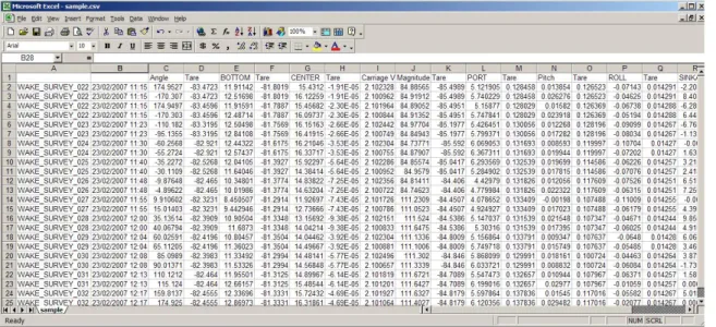
For more intense analysis purposes, once the segment selection on each file has been completed, it might be beneficial to view the raw data that has been selected. CSV files can be viewed in simple applications like Notepad or WordPad, but work best when opened through Microsoft Excel. Enclosed in the CSV file as shown in Figure 5 is a listing of filenames, acquisition dates and times, as well as the tared data on each channel for that segment.

Also included, but not shown, is a velocity data file that is produced once the velocity graphs appear. This file has the data sorted (and rounded) by radius and by ascending

(14)

angle measure, with corresponding values for axial, tangential, and radial velocity for each point.

Figure 5. Sample CSV Raw Data File

2.3 Additional Notes

During testing, it is common to experience difficulties with equipment during acquisition to the point where the DAC file created may be of no use in analysis. If this happens to be the case, the user can simply select one segment during a segment selection session, and doing this will not enter undesired data into the raw data file nor add

additional data to the resulting graph. However, the user should take note of the fact that this file may reappear if analysis is looped or rerun at any point in time unless the file is deleted from the test directory.

Also, it is important to not have the raw data file open while performing segment selecting. This will cause SWEET to throw the user a file permissions error.

3 - DESIGN

(15)

The basic structure of the module is laid out into many separate functions, two of which are common to all SWEET templates, while the others are placed in for simplification of mathematical computation and maintenance.

This document will give the overall breakdown of the entire body of code that composes WakeSurvey. Wherever possible, comments have been used to simplify and to explain function or assignment objectives.

3.2 Requirements

The WakeSurvey template was designed to meet a complete set of specifications. These specifications include:

• Given a specific file directory, to search and find files for a given base name, which have not been analyzed.

• Analyze these files through an interactive segment select unit. • Tare the data selected through the segment selector.

• Create two new channels for easier analysis: Position Magnitude (mm) & Angle (degrees)

• Output all data (both tare and test segments) marked by filename and date acquired to a comma separated values (CSV) file

• Use this CSV file to calculate yaw and pitch angles using Q, R, and PCal contour plots.

• From these yaw and pitch angles, calculate all velocity components

• Using these components plot graphs where data points have been sorted by position magnitude (or radius) and by increasing angle measure.

(16)

As Figure 6 below shows the structure of the WakeSurvey template using the UML guidelines. C_eqn inBetween defineparameters do run_analysis graph_check plot_graph reanalysis_mode graph_interval analysis_count csv_new filename head_correct_factor WakeSurvey

Figure 6. UML class diagram of WakeSurvey template.

3.4 The WakeSurvey Module

The WakeSurvey module is the only class in the template. This module performs all the necessary functions through the five methods listed above. Two of these methods are common to all SWEET templates; however, the other three have been implemented for simpler reading and comprehension for future developers. The other two functions shown at the bottom of the UML diagram are two basic functions that are called sparingly during execution. The following is a list of methods and attributes invoked by the WakeSurvey class:

(17)

Methods

o defineParameters - A method common to all SWEET templates. The variables inputted here are shown in the “Run Set Settings” window.

o do - Another method common to all SWEET templates. This method is what is executed when the user selects “Run” from the “Run Set Run” window. Here, the method performs a check to see whether a CSV file has already been created previously, and uses this information to determine whether to simply analyze every matching file with the user inputted base name, or whether to view the CSV file and check more thoroughly.

o run_analysis – This method is invoked when a file is to be analyzed. The DAC file is imported, an interactive segment select is introduced, and the selected data is written to the CSV file.

o graph_check – This boolean method simply checks to see whether it is appropriate to execute the following method, plot_graph.

o plot_graph – This method uses the data in the CSV file, calculates yaw and pitch angles for each point, and uses these values to find velocity components. It then sorts the components by radius and by ascending angle measure to produce a plot.

Attributes

o reanalysis_mode – If set to ‘True’, the template will analyze every file until the graphing routine is implemented.

o graph_interval – This attribute is determined by what the user inputs in the “show_graph_after_number_runs” field. If set to 0, this attribute will be set to –1. o analysis_count – This attribute begins at zero and iterates when a file is analyzed.

This continues until graph_check passes or all the files are analyzed.

o csv_new – This attribute is a bool that simply tells whether a CSV file for this run set already exists or not.

o filename – Equivalent to what the user inputs in the “CSV_name” field. o head_correct_factor – Equivalent to what the user inputs into the field of the

(18)

4 CONCLUSION

4.1 Recommendations

Possible recommendations for future updates to this template would include possibly implementing a real-time RUN file GUI for the user as analysis is completing. Also, a complete, interactive data fairing package where data points on the resulting velocity component graphs are movable so that a proper spline curve can be produced.

(19)

Appendix A: Source Code

sweet_cmd_options = r'--vms' import matplotlib

matplotlib.use('WXAgg') import wx

from sweet.template import Template from sweet.environment import environment from sweet.toolbox import Toolbox

import csv import numpy import glob

(20)

import os import math import logging from pylab import *

class WakeSurvey(Template):

"""

This script does the following:

- Reads a .DAC file (Or a batch of .DAC files) in a single directory - Plots four channels for viewing.

- Allows for interactive segment selection.

- Tares all segments (except YPos, XPos, Magnitude, and Angle).

- Constructs two new channels from existing channels: Angle & Magnitude - Places filename along with tared values into a .CSV file for easy analysis. - Graphs the .DAC files in terms of Vx/Vs & Vt/Vs with respect to angle. - Outputs velocity data to a .CSV file

""" def defineParameters(self): """

* reanalysis_mode = Reanalysis Mode (True or False) """ self.reanalysis_mode = False def do(self, CSV_name = "", dac_base_name = "", dac_file_directory = "", show_graph_after_number_runs = 0, head_correct_factor = 1.00 ): """

(21)

* CSV_name = CSV File Name

* Leave blank to output to a file with the same name as the DAC * file, but with a CSV extension.

* dac_base_name = .DAC Base Filename (Without Sequence Number) * dac_file_directory = .DAC File Directory

* show_graph_after_number_runs = Plot Data After Set Number of Analyzed Runs. (0 Will Only Show Plot At Finish)

* head_correct_factor = Multiplication Factor for Raw Pressure Data in Analysis. (1.00 Is Default)

"""

# Graph Interval is number of runs processed before updating & showing Vx/Vs and Vt/Vs plots.

if (show_graph_after_number_runs == 0): self.graph_interval = -1

else:

self.graph_interval = float(show_graph_after_number_runs) # Analysis count will iterate for every DAC file analyzed. self.analysis_count = 0

if CSV_name == "": CSV_name = dac_base_name + ".CSV"

# Directory name precaution. if dac_file_directory.endswith("\\") == False: dac_file_directory += "\\"

# Checking to see if .CSV file exists. if CSV_name in os.listdir(os.getcwd()): check_file = True else: check_file = False self.CSV_name = CSV_name self.head_correct_factor = head_correct_factor filelist = glob.glob(dac_file_directory + "\\" + dac_base_name + "*.DAC")

# Checking already created .CSV file for files in filelist. # Flag is raised when .DAC file has already been analyzed.

(22)

flag = False if check_file:

# Write previously analyzed filenames to a list. self.csv_new = False

f = open(self.CSV_name,"r") reader = csv.reader(f) run_names = [] for row in reader:

run_names.append(row[0]) f.close()

for note in filelist: flag = False

for entries in run_names:

if dac_file_directory + entries + ".DAC" == note: flag = True if flag == False: self.run_analysis(note) self.analysis_count+=1 if self.graph_check(): self.plot_graph() return else: if self.reanalysis_mode == False:

logging.info(note + " has already been analyzed.") else: self.run_analysis(note) self.analysis_count+=1 if self.graph_check(): self.plot_graph() return self.plot_graph() else: self.csv_new = True if filelist:

for note in filelist: self.run_analysis(note) self.csv_new = False self.analysis_count+=1 if self.graph_check(): self.plot_graph() return self.plot_graph()

(23)

def run_analysis(self,dac_file_name): tb = Toolbox() dac_file = tb.dac_file(dac_file_name)

# Read the DAC file, without including Carriage Positon. channels = dac_file.read(exclude=["Carriage position", "TUG TRIM"])

channels.rename("roll","ROLL")

channels.rename("BARGE HEAVE","SINKAGE") channels.rename("BARGE PITCH","Pitch")

# Create two new channels 'Angle' & 'Magnitude' for each segment. # This angle measure is using the positive x-axis as its reference.

channels["Angle"] = tb.channel(y_name = "Angle", y_units = "Degrees",

delta_x = channels["XPos"])

channels["Angle"].data =

(numpy.arctan2(channels["YPos"].data,channels["XPos"].data)*(180/math.pi)) channels["Magnitude"] = tb.channel(y_name = "Magnitude",

y_units = "mm",

delta_x = channels["XPos"]) channels["Magnitude"].data =

numpy.sqrt(pow(channels["YPos"].data,2)+pow(channels["XPos"].data,2))

# Start an instance of the segment selector class selector = tb.segment_selector()

selector.interactive_mode = True

selector.channels_to_display = ["Carriage Velocity", "CENTER","YPos","XPos"] segments = selector.select(channels)

tare_segment = segments[0].clone()

# Tare each segment EXCEPT the first segment.

# Tare each channel EXCEPT YPos, XPos, Magnitude, & Angle.

(24)

segment.tare(tare_segment, exclude=["YPos","XPos","Magnitude","Angle"]) # In order to get tare segment back, use clone.

segments[0] = tare_segment.clone()

# Start each row with the filename and acquisition date.

# Remaining channels & segments will be tared in subsequent rows.

keys = segment.keys() keys.sort()

row = [channels.DAC_TEST_NAME,str(channels.DAC_START_TIME)] column_count = 0

# Add column headers if .CSV not previously created if self.csv_new == True:

f = open(self.CSV_name, "wb") writer = csv.writer(f)

# For a new CSV, the first two elements of the first row are blank (purely cosmetic). row = ["",""]

for key in keys:

if key not in ["Angle","XPos","YPos","Magnitude"]:

row.append( "Tare" + "\n" '%s' % (segment[key].channel_name[1])) row.append( '%s' % (segment[key].channel_name[1])) writer.writerow(row) else: f = open(self.CSV_name, "ab") writer = csv.writer(f)

# Cycle through each channel of each segment, writing each segment as a row in the .CSV file for segment in segments:

for key in keys: column_count += 1

# Tare segment data for each channel listed immediately before real data. if key not in ["Angle","XPos","YPos","Magnitude"]:

row.append(tare_segment[key].data.mean()) if key in ["Angle"]:

row.append(segment[key].data.mean()*-1) else:

(25)

row.append(segment[key].data.mean()) if ((column_count % 13) == 0):

# Condition allowing all segments after tare segment to be written to .CSV if (column_count > 13):

writer.writerow(row)

row = [channels.DAC_TEST_NAME,str(channels.DAC_START_TIME)] f.close()

# Simple check to see whether .CSV file should be analyzed. def graph_check(self): if self.graph_interval == self.analysis_count: return True else: return False def plot_graph(self): f = open(self.CSV_name,"rb") reader = csv.reader(f) d = open("WksCal.txt","rb") data_in = csv.reader(d,delimiter="\t") q_calc, r_calc = [],[]

# Imported values from .CSV file

top, port, stbd, bottom, magnitude, center, angle, c_vel = [], [], [], [], [], [], [], [] # Imported values from wake contour text file

q, r, yaw , pitch, pcal = [], [], [], [], []

# Calculated values of pitch and yaw for each segment pitch_f, yaw_f, CP_bar = [],[],[]

# All calculated velocity components have their own lists

# This is to make export simpler in case of calculation issues/errors. V_x, V_y, V_z, V_t, V_r, V = [], [], [], [], [], []

cnt = -2 dim = 81 row = -1

for line in data_in: if cnt >= 0:

(26)

yaw.append([]) pitch.append([]) pcal.append([]) r.append([]) q.append([]) row += 1 yaw[row].append(float(line[0])) pitch[row].append(float(line[1])) pcal[row].append(float(line[2])) q[row].append(float(line[3])) r[row].append(float(line[4])) cnt += 1 d.close() count = -1 for line in reader: if line[2] == "": break if count >= 0: top.append(float(line[21])*self.head_correct_factor) center.append(float(line[6])*self.head_correct_factor) port.append(float(line[11])*self.head_correct_factor) bottom.append(float(line[4])*self.head_correct_factor) stbd.append(float(line[19])*self.head_correct_factor) c_vel.append(float(line[8])) angle.append(float(line[2])) magnitude.append(float(line[9])) count += 1 f.close() for i in range(len(top)): q_calc.append(C_eqn(stbd[i],c_vel[i]) - C_eqn(port[i],c_vel[i])) r_calc.append(C_eqn(bottom[i],c_vel[i]) - C_eqn(top[i],c_vel[i])) CP_bar.append((C_eqn(port[i],c_vel[i]) + C_eqn(stbd[i],c_vel[i]) + C_eqn(top[i],c_vel[i]) + C_eqn(bottom[i],c_vel[i]))/4.0) for i in range(len(q_calc)): dmin = 25 for t in range(80): for j in range(80): xd = q_calc[i] - q[t][j] yd = r_calc[i] - r[t][j] if xd >= 0 and yd >= 0:

dist = math.sqrt(xd**2 + yd**2) if dist < dmin:

(27)

dmin = dist k = t l = j

## find where contours intersects grid ii = [0, 0, 1, 1, 0] jj = [0, 1, 1, 0, 0] x = [] y = [] xr = [] yr = [] for cnt in range(4): i1 = k + ii[cnt] i2 = k + ii[cnt+1] j1 = l + jj[cnt] j2 = l + jj[cnt+1]

if inBetween(q[i1][j1], q_calc[i], q[i2][j2]):

per = (q_calc[i] - q[i1][j1]) / (q[i2][j2] - q[i1][j1]) x.append(yaw[i1][j1] + per*(yaw[i2][j2]-yaw[i1][j1]) ) y.append(pitch[i1][j1] + per*(pitch[i2][j2]-pitch[i1][j1]) ) if inBetween(r[i1][j1], r_calc[i], r[i2][j2]):

per = (r_calc[i] - r[i1][j1]) / (r[i2][j2] - r[i1][j1]) xr.append(yaw[i1][j1] + per*(yaw[i2][j2]-yaw[i1][j1]) ) yr.append(pitch[i1][j1] + per*(pitch[i2][j2]-pitch[i1][j1]) ) while len(x) < 2: x.append((yaw[i1][j1]+yaw[i2][j2])/2) y.append((pitch[i1][j1]+pitch[i2][j2])/2) if len(y) < 2: xr.append((yaw[i1][j1]+yaw[i2][j2])/2) yr.append((pitch[i1][j1]+pitch[i2][j2])/2)

## check for double corner values st = 0

while len(x) > 2:

for i in range(st+1,len(x)):

if x[st] == x[i] and y[st] == y[i]: x.remove(x[st]) y.remove(y[st]) st +=1 st = 0 while len(xr) > 2: for q in range(st+1,len(xr)):

(28)

if xr[st] == xr[q] and yr[st] == yr[q]: xr.remove(xr[st]) yr.remove(yr[st]) st += 1 x.extend(xr) y.extend(yr)

## find intersection of two contour lines

denom = (y[3]-y[2])*(x[1]-x[0])-(x[3]-x[2])*(y[1]-y[0]) ## check if denom zero, then yaw and pitch are x[0] y[0] if abs(denom) <= 0.00001:

ua = 0.5 else:

ua = ((x[3]-x[2])*(y[0]-y[2]) - (y[3]-y[2])*(x[0]-x[2])) / denom if ua > 1:

ua = 0.5

yaw_f.append(x[0] + ua*(x[1]-x[0])) pitch_f.append(y[0] + ua*(y[1]-y[0]))

# components used in velocity calculation.

p_up = pcal[l][k] + ((pcal[l][k+1] - pcal[l][k])*(pitch_f[i]-pitch[l][k]))/(pitch[l+1][k]-pitch[l][k]) p_down = pcal[l+1][k] + ((pcal[l+1][k+1] -

pcal[l+1][k])*(pitch_f[i]-pitch[l][k+1]))/(pitch[l+1][k+1]-pitch[l][k+1])

po = p_up + (p_down - p_up)*(yaw_f[i]-yaw[l][k])/(yaw[l][k+1] - yaw[l][k]) V.append(pow(((C_eqn(center[i],c_vel[i]) - CP_bar[i])/po),2)*c_vel[i]) V_x.append(V[i]*math.cos(math.radians(pitch_f[i]))*(math.cos(math.radians(yaw_f[i])))) V_y.append(V[i]*math.cos(math.radians(pitch_f[i]))*(math.sin(math.radians(yaw_f[i])))) V_z.append(V[i]*math.sin(math.radians(pitch_f[i]))) V_t.append((-1*V_y[i]*math.cos(math.radians(angle[i])))-(V_z[i]*math.sin(math.radians(angle[i])))) V_r.append(V_y[i]*math.sin(math.radians(angle[i]))-V_z[i]*math.cos(math.radians(angle[i]))) # Round magnitude values that were slightly off to one set value.

(29)

# Velocities exist in a dictionary whereby the keys are radii # and the values for each key are four corresponding lists:

# 1) V_x/V_s 2) V_t/V_s 3) V_r/V_s 4) V_y/V_s 5) V_z/V_s 6) Angle d = {}

rounding_list = [] for i in range(len(c_vel)): match = False

# if a rounded magnitude happens to already exist in a key rounding_list.append(round(magnitude[i]-(magnitude[i]*.1))) rounding_list.append(round((magnitude[i]*.1)+magnitude[i])) for key in d.keys():

if inBetween(rounding_list[0],key,rounding_list[1]): match = True k = key if match: d[k][0].append(V_x[i]/c_vel[i]) d[k][1].append(V_t[i]/c_vel[i]) d[k][2].append(V_r[i]/c_vel[i]) d[k][3].append(V_y[i]/c_vel[i]) d[k][4].append(V_z[i]/c_vel[i]) d[k][5].append(angle[i]) rounding_list = [] else: Vx_vs = [] Angle = [] Vt_vs = [] Vr_vs = [] Vz_vs = [] Vy_vs = [] d[round(magnitude[i])] = Vx_vs,Vt_vs,Vr_vs,Vy_vs,Vz_vs,Angle Vx_vs.append(V_x[i]/c_vel[i]) Vt_vs.append(V_t[i]/c_vel[i]) Angle.append(angle[i]) Vr_vs.append(V_r[i]/c_vel[i]) Vy_vs.append(V_y[i]/c_vel[i]) Vz_vs.append(V_z[i]/c_vel[i]) rounding_list = []

# Sort values by ascending angle so proper lines can be drawn between them when plotted # Completed by copying lists and comparing values.

for key in d.keys(): a = list(d[key][0]) b = list(d[key][1])

(30)

c = list(d[key][2]) e = list(d[key][3]) f = list(d[key][4]) g = list(d[key][5]) d[key][5].sort()

for t, value in enumerate(d[key][5]): for j, number in enumerate(g): if value == number: d[key][0][t] = a[j] d[key][1][t] = b[j] d[key][2][t] = c[j] d[key][3][t] = e[j] d[key][4][t] = f[j] d[key][5][t] = g[j]

# Print the velocity results to a .CSV file

titles = ["Vx_vs","Vt_vs","Vr_vs","Vy_vs","Vz_vs","Angle","Radius"] row = []

results_filename = "velocity_" + self.CSV_name g = open(results_filename,"wb") writer = csv.writer(g) for t in titles: row.append(t) writer.writerow(row) row = []

for key in d.keys():

for n in range(len(d[key][2])): for l in range(6): row.append(d[key][l][n]) row.append(key) writer.writerow(row) row=[] g.close() color = ["bo-","co-","ko-","go-","ro-"] cnt = 0

# Show two subplots of the velocity data.

# If a particular radius ratio has less than 5 points, do not plot it. for key in d.keys():

(31)

del d[key]

subplot(211) for key in d.keys():

plot(d[key][5],d[key][0],color[cnt]) cnt += 1

grid(True)

title("Wake Survey Analysis: Velocity Plots",bbox={'facecolor':'0.9', 'pad':5}) xlabel(r"$\theta \rm{(degrees)}$")

ylabel(r"$\ v_x/v_s $") cnt=0

subplot(212) for key in d.keys():

plot(d[key][5],d[key][1],color[cnt]) cnt += 1 grid(True) xlabel(r"$\theta \rm{(degrees)}$") ylabel(r"$\ v_t/v_s$") window = get_current_fig_manager().window window.Show(True)

# Simple function for contour checking. def inBetween(a,b,c):

if (a >= b >= c) or (a <= b <= c): return True

else:

return False

# Pressure co-effcient equation def C_eqn(pressure,velocity):

return ((9.80665*pressure))/(50*pow(velocity,2))

if __name__ == '__main__':

WakeSurvey().do(*environment.arguments, **environment.keyword_arguments)

(32)

In the following segment, the process behind using raw pressure values from each of the five transducers and finding such results as yaw and pitch angles and velocity

components will be documented.

From the raw pressure data, each of the five transducers relates to a probe coefficient, CPn. Transducer Location n Top 1 Starboard 2 Bottom 3 Port 4 Center 5

The CPn coefficient is calculated by:

50 gP 2 n s Pn C ν =

where: CPn = Pressure coefficient

g = acceleration due to gravity (9.80665m/s2) νS = carriage velocity (m/s) Followed by: 4 C C C C CP_Bar P1 P2 P3 P4 + + + =

From this, dimensionless coefficients sensitive to the yaw and pitch angles, called Q and R respectively will be calculated as well as a PFlow.

Q = CP2 – CP4 R = CP3 – CP1 PFlow = CP5 – CP_Bar

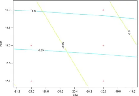
To compute the yaw and pitch angles of the incoming flow onto the pitot tube, a linear contouring intersection method is used based on tables (matrices) of Q, R, Pitch and Yaw values defined from pitot tube calibration. (These Q and R matrix values will be referred

(33)

to as QT and RT from here onward.). In order to for this procedure to function properly, QT (x) and RT (y) are plotted as contour lines over Pitch and Yaw angles in the

calibration matrix. (Shown in Figure 7). The calculated values of Q and R are then compared with each of the values of QT and RT until a QT, RT point is found that is closest to the original Q, R point. This is completed to find a relative area to where Q and R exist in the plot and in doing this, the point can be surrounded by calculated yaw and pitch values in order to get a good estimate of where the QT and RT contour lines are. At this time, the 4 values in the both QT and RT matrices surrounding this point are

compared to estimate where the contour lines pass through. Furthermore, a linear

estimate then can be made to determine the location of an intersection point between the two contour lines. From this intersection point, the yaw and pitch angles are derived.

Figure 7. A close-up of a contour plot of Q and R against Pitch and Yaw. The red marks are yaw and pitch plotted against each other. The green contour line represents Q values, while the blue contour line represents R values.

Once the yaw and pitch values are known, the magnitude of the flow is found using interpolation methods in the PCal table which overlays the pitch and yaw plot. Three elements are calculated from this PCal table: Pup, Pdown, and Po. (Where Pup is an interpolation across the top row, Pdown an interpolation across the bottom row, and Po across the columns) Using the same co-ordinates for the “square” shape created for finding yaw and pitch angles, Po is found, which determines the magnitude of flow. See

(34)

the source code in Appendix A for an exact definition of the interpolation. The most important thing to note is:

s o Flow P P _ν ν _⎜⎜ ⋅ ⎝ ⎛ ⎟⎟ ⎠ ⎞ = 2

From the velocity equation above and the previously found pitch and yaw angles, the remaining components can be found.

) sin( ) cos(θ ν θ ν ν_t =− _y − _z ) cos( ) cos(β ψ ν ν_x = ⋅ ⋅ ) cos( ) sin(θ ν θ ν ν_r = _y − _z ) sin( ) cos(β ψ ν ν_y = ⋅ ⋅ ) sin(β ν ν_z = ⋅ where: ψ = yaw angle