HAL Id: hal-03101212
https://hal.archives-ouvertes.fr/hal-03101212
Submitted on 11 Jan 2021
HAL is a multi-disciplinary open access
archive for the deposit and dissemination of
sci-entific research documents, whether they are
pub-lished or not. The documents may come from
teaching and research institutions in France or
abroad, or from public or private research centers.
L’archive ouverte pluridisciplinaire HAL, est
destinée au dépôt et à la diffusion de documents
scientifiques de niveau recherche, publiés ou non,
émanant des établissements d’enseignement et de
recherche français ou étrangers, des laboratoires
publics ou privés.
paleoclimate data, climate modeling, and modern
observations that 2 °C global warming could be
dangerous
James Hansen, Makiko Sato, Paul Hearty, Reto Ruedy, Maxwell Kelley,
Valerie Masson-Delmotte, Gary Russell, George Tselioudis, Junji Cao, Eric
Rignot, et al.
To cite this version:
James Hansen, Makiko Sato, Paul Hearty, Reto Ruedy, Maxwell Kelley, et al.. Ice melt, sea level rise
and superstorms: evidence from paleoclimate data, climate modeling, and modern observations that
2 °C global warming could be dangerous. Atmospheric Chemistry and Physics, European Geosciences
Union, 2016, 16 (6), pp.3761-3812. �10.5194/ACP-16-3761-2016�. �hal-03101212�
www.atmos-chem-phys.net/16/3761/2016/ doi:10.5194/acp-16-3761-2016
© Author(s) 2016. CC Attribution 3.0 License.
Ice melt, sea level rise and superstorms: evidence from paleoclimate
data, climate modeling, and modern observations that 2
◦
C global
warming could be dangerous
James Hansen1, Makiko Sato1, Paul Hearty2, Reto Ruedy3,4, Maxwell Kelley3,4, Valerie Masson-Delmotte5,
Gary Russell4, George Tselioudis4, Junji Cao6, Eric Rignot7,8, Isabella Velicogna7,8, Blair Tormey9, Bailey Donovan10, Evgeniya Kandiano11, Karina von Schuckmann12, Pushker Kharecha1,4, Allegra N. Legrande4, Michael Bauer4,13, and Kwok-Wai Lo3,4
1Climate Science, Awareness and Solutions, Columbia University Earth Institute, New York, NY 10115, USA 2Department of Environmental Studies, University of North Carolina at Wilmington, NC 28403, USA 3Trinnovium LLC, New York, NY 10025, USA
4NASA Goddard Institute for Space Studies, 2880 Broadway, New York, NY 10025, USA
5Institut Pierre Simon Laplace, Laboratoire des Sciences du Climat et de l’Environnement (CEA-CNRS-UVSQ),
Gif-sur-Yvette, France
6Key Lab of Aerosol Chemistry & Physics, Institute of Earth Environment, Chinese Academy of Sciences,
Xi’an 710075, China
7Jet Propulsion Laboratory, California Institute of Technology, Pasadena, CA 91109, USA 8Department of Earth System Science, University of California, Irvine, CA 92697, USA
9Program for the Study of Developed Shorelines, Western Carolina University, Cullowhee, NC 28723, USA 10Department of Geological Sciences, East Carolina University, Greenville, NC 27858, USA
11GEOMAR, Helmholtz Centre for Ocean Research, Wischhofstrasse 1–3, Kiel 24148, Germany 12Mediterranean Institute of Oceanography, University of Toulon, La Garde, France
13Department of Applied Physics and Applied Mathematics, Columbia University, New York, NY 10027, USA
Correspondence to: James Hansen (jeh1@columbia.edu)
Received: 11 June 2015 – Published in Atmos. Chem. Phys. Discuss.: 23 July 2015 Revised: 17 February 2016 – Accepted: 18 February 2016 – Published: 22 March 2016
Abstract. We use numerical climate simulations, paleocli-mate data, and modern observations to study the effect of growing ice melt from Antarctica and Greenland. Meltwa-ter tends to stabilize the ocean column, inducing amplifying feedbacks that increase subsurface ocean warming and ice shelf melting. Cold meltwater and induced dynamical effects cause ocean surface cooling in the Southern Ocean and North Atlantic, thus increasing Earth’s energy imbalance and heat flux into most of the global ocean’s surface. Southern Ocean surface cooling, while lower latitudes are warming, increases precipitation on the Southern Ocean, increasing ocean strat-ification, slowing deepwater formation, and increasing ice sheet mass loss. These feedbacks make ice sheets in contact with the ocean vulnerable to accelerating disintegration. We
hypothesize that ice mass loss from the most vulnerable ice, sufficient to raise sea level several meters, is better approx-imated as exponential than by a more linear response. Dou-bling times of 10, 20 or 40 years yield multi-meter sea level rise in about 50, 100 or 200 years. Recent ice melt doubling times are near the lower end of the 10–40-year range, but the record is too short to confirm the nature of the response. The feedbacks, including subsurface ocean warming, help explain paleoclimate data and point to a dominant Southern Ocean role in controlling atmospheric CO2, which in turn
ex-ercised tight control on global temperature and sea level. The millennial (500–2000-year) timescale of deep-ocean ventila-tion affects the timescale for natural CO2 change and thus
level changes, but this paleo-millennial timescale should not be misinterpreted as the timescale for ice sheet response to a rapid, large, human-made climate forcing. These climate feedbacks aid interpretation of events late in the prior in-terglacial, when sea level rose to +6–9 m with evidence of extreme storms while Earth was less than 1◦C warmer than today. Ice melt cooling of the North Atlantic and Southern oceans increases atmospheric temperature gradients, eddy kinetic energy and baroclinicity, thus driving more power-ful storms. The modeling, paleoclimate evidence, and on-going observations together imply that 2◦C global warming above the preindustrial level could be dangerous. Continued high fossil fuel emissions this century are predicted to yield (1) cooling of the Southern Ocean, especially in the Western Hemisphere; (2) slowing of the Southern Ocean overturning circulation, warming of the ice shelves, and growing ice sheet mass loss; (3) slowdown and eventual shutdown of the lantic overturning circulation with cooling of the North At-lantic region; (4) increasingly powerful storms; and (5) non-linearly growing sea level rise, reaching several meters over a timescale of 50–150 years. These predictions, especially the cooling in the Southern Ocean and North Atlantic with markedly reduced warming or even cooling in Europe, dif-fer fundamentally from existing climate change assessments. We discuss observations and modeling studies needed to re-fute or clarify these assertions.
1 Introduction
Humanity is rapidly extracting and burning fossil fuels with-out full understanding of the consequences. Current assess-ments place emphasis on practical effects such as increas-ing extremes of heat waves, droughts, heavy rainfall, floods, and encroaching seas (IPCC, 2014; USNCA, 2014). These assessments and our recent study (Hansen et al., 2013a) con-clude that there is an urgency to slow carbon dioxide (CO2)
emissions, because the longevity of the carbon in the climate system (Archer, 2005) and persistence of the induced warm-ing (Solomon et al., 2010) may lock in unavoidable, highly undesirable consequences.
Despite these warnings, fossil fuels remain the world’s pri-mary energy source and global CO2 emissions continue at
a high level, perhaps with an expectation that humanity can adapt to climate change and find ways to minimize effects via advanced technologies. We suggest that this viewpoint fails to appreciate the nature of the threat posed by ice sheet insta-bility and sea level rise. If the ocean continues to accumulate heat and increase melting of marine-terminating ice shelves of Antarctica and Greenland, a point will be reached at which it is impossible to avoid large-scale ice sheet disintegration with sea level rise of at least several meters. The economic and social cost of losing functionality of all coastal cities is practically incalculable. We suggest that a strategy relying
on adaptation to such consequences will be unacceptable to most of humanity, so it is important to understand this threat as soon as possible.
We investigate the climate threat using a combination of atmosphere–ocean modeling, information from paleoclimate data, and observations of ongoing climate change. Each of these has limitations: modeling is an imperfect representa-tion of the climate system, paleo-data consist mainly of proxy climate information usually with substantial ambiguities, and modern observations are limited in scope and accuracy. How-ever, with the help of a large body of research by the scientific community, it is possible to draw meaningful conclusions.
2 Background information and organization of the paper
Our study germinated a decade ago. Hansen (2005, 2007) ar-gued that the modest 21st century sea level rise projected by IPCC (2001), less than a meter, was inconsistent with pre-sumed climate forcings, which were larger than paleoclimate forcings associated with sea level rise of many meters. His argument about the potential rate of sea level rise was nec-essarily heuristic, because ice sheet models are at an early stage of development, depending sensitively on many pro-cesses that are poorly understood. This uncertainty is illus-trated by Pollard et al. (2015), who found that addition of hydro-fracturing and cliff failure into their ice sheet model increased simulated sea level rise from 2 to 17 m, in response to only 2◦C ocean warming and accelerated the time for sub-stantial change from several centuries to several decades.
The focus for our paper developed in 2007, when the first author (JH) read several papers by co-author P. Hearty. Hearty used geologic field data to make a persuasive case for rapid sea level rise late in the prior interglacial period to a height +6–9 m relative to today, and he presented evidence of strong storms in the Bahamas and Bermuda at that time. Hearty’s data suggested violent climate behavior on a planet only slightly warmer than today.
Our study was designed to shed light on, or at least raise questions about, physical processes that could help account for the paleoclimate data and have relevance to ongoing and future climate change. Our assumption was that extraction of significant information on these processes would require use of and analysis of (1) climate modeling, (2) paleoclimate data, and (3) modern observations. It is the combination of all of these that helps us interpret the intricate paleoclimate data and extract implications about future sea level and storms.
Our approach is to postulate existence of feedbacks that can rapidly accelerate ice melt, impose such rapidly grow-ing freshwater injection on a climate model, and look for a climate response that supports such acceleration. Our im-posed ice melt grows nonlinearly in time, specifically expo-nentially, so the rate is characterized by a doubling time. To-tal amounts of freshwater injection are chosen in the range
1–5 m of sea level, amounts that can be provided by vulner-able ice masses in contact with the ocean. We find signif-icant impact of meltwater on global climate and feedbacks that support ice melt acceleration. We obtain this informa-tion without use of ice sheet models, which are still at an early stage of development, in contrast to global general cir-culation models that were developed over more than half a century and do a capable job of simulating atmosphere and ocean circulation.
Our principal finding concerns the effect of meltwater on stratification of the high-latitude ocean and resulting ocean heat sequestration that leads to melting of ice shelves and catastrophic ice sheet collapse. Stratification contrasts with homogenization. Winter conditions on parts of the North At-lantic Ocean and around the edges of Antarctica normally produce cold, salty water that is dense enough to sink to the deep ocean, thus stirring and tending to homogenize the wa-ter column. Injection of fresh meltwawa-ter reduces the density of the upper ocean wind-stirred mixed layer, thus reducing the rate at which cold surface water sinks in winter at high latitudes. Vertical mixing normally brings warmer water to the surface, where heat is released to the atmosphere and space. Thus the increased stratification due to freshwater in-jection causes heat to be retained at ocean depth, where it is available to melt ice shelves. Despite improvements that we make in our ocean model, which allow Antarctic Bottom Water to be formed at proper locations, we suggest that ex-cessive mixing in many climate models, ours included, lim-its this stratification effect. Thus, human impact on ice sheets and sea level may be even more imminent than in our model, suggesting a need for confirmatory observations.
Our paper published in Atmospheric Chemistry and Physics Discussion was organized in the chronological order of our investigation. Here we reorganize the work to make the science easier to follow. First, we describe our climate simulations with specified growing freshwater sources in the North Atlantic and Southern oceans. Second, we analyze pa-leoclimate data for evidence of these processes and possible implications for the future. Third, we examine modern data for evidence that the simulated climate changes are already occurring.
We use paleoclimate data to find support for and deeper understanding of these processes, focusing especially on events in the last interglacial period warmer than today, called Marine Isotope Stage (MIS) 5e in studies of ocean sediment cores, Eemian in European climate studies, and sometimes Sangamonian in US literature (see Sect. 4.2 for timescale diagram of marine isotope stages). Accurately known changes of Earth’s astronomical configuration altered the seasonal and geographical distribution of incoming ra-diation during the Eemian. Resulting global warming was due to feedbacks that amplified the orbital forcing. While the Eemian is not an analog of future warming, it is useful for investigating climate feedbacks, including the interplay between ice melt at high latitudes and ocean circulation.
3 Simulations of 1850–2300 climate change
We make simulations for 1850–2300 with radiative forcings that were used in CMIP (Climate Model Intercomparison Project) simulations reported by IPCC (2007, 2013). This al-lows comparison of our present simulations with prior stud-ies. First, for the sake of later raising and discussing funda-mental questions about ocean mixing and climate response time, we define climate forcings and the relation of forcings to Earth’s energy imbalance and global temperature. 3.1 Climate forcing, Earth’s energy imbalance, and
climate response function
A climate forcing is an imposed perturbation of Earth’s en-ergy balance, such as change in solar irradiance or a ra-diatively effective constituent of the atmosphere or surface. Non-radiative climate forcings are possible, e.g., change in Earth’s surface roughness or rotation rate, but these are small and radiative feedbacks likely dominate global climate re-sponse even in such cases. The net forcing driving climate change in our simulations (Fig. S16 in the Supplement) is almost 2 W m−2 at present and increases to 5–6 W m−2 at the end of this century, depending on how much the (nega-tive) aerosol forcing is assumed to reduce the greenhouse gas (GHG) forcing. The GHG forcing is based on IPCC scenario A1B. “Orbital” forcings, i.e., changes in the seasonal and ge-ographical distribution of insolation on millennial timescales caused by changes of Earth’s orbit and spin axis tilt, are near zero on global average, but they spur “slow feedbacks” of several W m−2, mainly change in surface reflectivity and
GHGs.
When a climate forcing changes, say solar irradiance in-creases or atmospheric CO2 increases, Earth is temporarily
out of energy balance, that is, more energy coming in than going out in these cases, so Earth’s temperature will increase until energy balance is restored. Earth’s energy imbalance is a result of the climate system’s inertia, i.e., the slowness of the surface temperature to respond to changing global cli-mate forcing. Earth’s energy imbalance is a function of ocean mixing, as well as climate forcing and climate sensitivity, the latter being the equilibrium global temperature response to a specified climate forcing. Earth’s present energy imbalance, +0.5–1 W m−2(von Schuckmann et al., 2016), provides an indication of how much additional global warming is still “in the pipeline” if climate forcings remain unchanged. How-ever, climate change generated by today’s energy imbalance, especially the rate at which it occurs, is quite different than climate change in response to a new forcing of equal mag-nitude. Understanding this difference is relevant to issues raised in this paper.
The different effect of old and new climate forcings is im-plicit in the shape of the climate response function, R(t ), where R is the fraction of the equilibrium global temper-ature change achieved as a function of time following
im-position of a forcing. Global climate models find that a large fraction of the equilibrium response is obtained quickly, about half of the response occurring within several years, but the remainder is “recalcitrant” (Held et al., 2010), requir-ing many decades or even centuries for nearly complete re-sponse. Hansen (2008) showed that once a climate model’s response function R is known, based on simulations for an instant forcing, global temperature change, T (t ), in response to any climate forcing history, F (t ), can be accurately ob-tained from a simple (Green’s function) integration of R over time:
T (t ) = Z
R(t )[dF /dt ]dt. (1)
dF / dt is the annual increment of the net forcing and the in-tegration begins before human-made climate forcing became substantial.
We use these concepts in discussing evidence that most ocean models, ours included, are too diffusive. Such exces-sive mixing causes the Southern and North Atlantic oceans in the models to have an unrealistically slow response to surface meltwater injection. Implications include a more imminent threat of slowdowns of Antarctic Bottom Water and North Atlantic Deep Water formation than present models suggest, with regional and global climate impacts.
3.2 Climate model
Simulations are made with an improved version of a coarse-resolution model that allows long runs at low cost: GISS (Goddard Institute for Space Studies) modelE-R. The atmo-sphere model is the documented modelE (Schmidt et al., 2006). The ocean is based on the Russell et al. (1995) model that conserves water and salt mass; has a free surface with divergent flow; uses a linear upstream scheme for advection; allows flow through 12 sub-resolution straits; and has back-ground diffusivity of 0.3 cm2s−1, resolution of 4◦×5◦and 13 layers that increase in thickness with depth.
However, the ocean model includes simple but significant changes, compared with the version documented in simula-tions by Miller et al. (2014). First, an error in the calculation of neutral surfaces in the Gent–McWilliams (GM; Gent and McWilliams, 1990) mesoscale eddy parameterization was corrected; the resulting increased slope of neutral surfaces provides proper leverage to the restratification process and correctly orients eddy stirring along those surfaces.
Second, the calculation of eddy diffusivity Kmesofor GM
following Visbeck et al. (1997) was simplified to use a length scale independent of the density structure (J. Marshall, per-sonal communication, 2012):
Kmeso=C/[TEady×f (latitude)], (2)
where C = (27.9 km)2, Eady growth rate 1/TEady= {|S × N |}, S is the neutral surface slope, N the Brunt–Väisälä
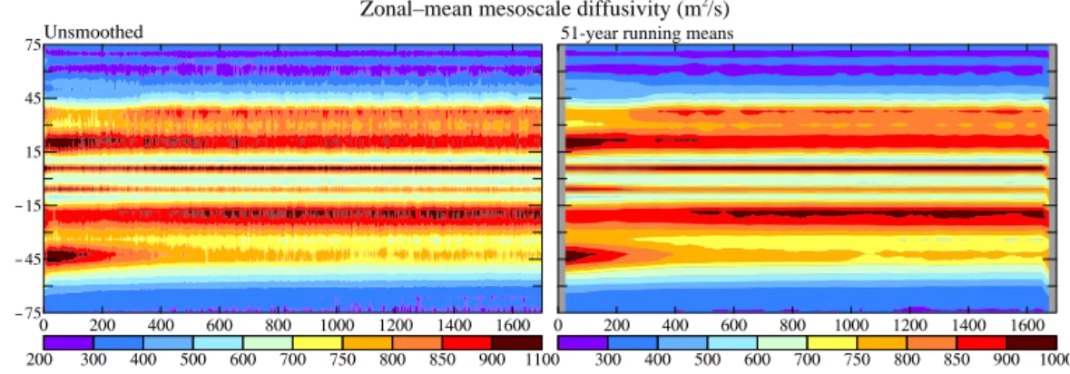
frequency, { } signifies averaging over the upper D me-ters of ocean depth, D = min(max(depth, 400 m), 1000 m), and f (latitude) = max(0.1, sin(|latitude|))1 to qualitatively mimic the larger values of the Rossby radius of deformation at low latitudes. These choices for Kmeso, whose simplicity is
congruent with the use of a depth-independent eddy diffusiv-ity and the use of 1/Teadyas a metric of eddy energy, result in
the zonal average diffusivity shown in Fig. 1. Third, the so-called nonlocal terms in the KPP mixing parameterization (Large et al., 1994) were activated. All of these modifica-tions tend to increase the ocean stratification, and in particu-lar the Southern Ocean state is fundamentally improved. For example, we show in Sect. 3.8.5 that our current model pro-duces Antarctic Bottom Water on the Antarctic coastline, as observed, rather than in the middle of the Southern Ocean as occurs in many models, including the GISS-ER model docu-mented in CMIP5. However, although overall realism of the ocean circulation is much improved, significant model defi-ciencies remain, as we will describe.
The simulated Atlantic meridional overturning circulation (AMOC) has maximum flux that varies within the range ∼14–18 Sv in the model control run (Figs. 2 and 3). AMOC strength in recent observations is 17.5 ± 1.6 Sv (Baringer et al., 2013; Srokosz et al., 2012), based on 8 years (2004– 2011) of data for an in situ mooring array (Rayner et al., 2011; Johns et al., 2011).
Ocean model control run initial conditions are climatology for temperature and salinity (Levitus and Boyer, 1994; Lev-itus et al., 1994); atmospheric composition is that of 1880 (Hansen et al., 2011). Overall model drift from control run initial conditions is moderate (see Fig. S1 for planetary en-ergy imbalance and global temperature), but there is drift in the North Atlantic circulation. The AMOC circulation cell initially is confined to the upper 3 km at all latitudes (1st cen-tury in Figs. 2 and 3), but by the 5th cencen-tury the cell reaches deeper at high latitudes.
Atmospheric and surface climate in the present model is similar to the documented modelE-R, but because of changes to the ocean model we provide several diagnostics in the Sup-plement. A notable flaw in the simulated surface climate is the unrealistic double precipitation maximum in the tropi-cal Pacific (Fig. S2). This double Intertropitropi-cal Convergence Zone (ITCZ) occurs in many models and may be related to cloud and radiation biases over the Southern Ocean (Hwang and Frierson, 2013) or deficient low level clouds in the trop-ical Pacific (de Szoeke and Xie, 2008). Another flaw is un-realistic hemispheric sea ice, with too much sea ice in the
1Where ocean depth exceeds 1000 m, these conditions yield
D =1000 m, thus excluding any first-order abyssal bathymetric im-print on upper ocean eddy energy, consistent with theory and ob-servations. The other objective of the stated condition is to limit release of potential energy in the few ocean gridboxes with ocean depth less than 400 m, because shallow depths limit the ability of baroclinic eddies to release potential energy via vertical motion.
Zonal–mean mesoscale diffusivity (m /s)
51-year running means
Figure 1. Zonal-mean mesoscale diffusivity (m2s−1) versus time in control run.
–25 –10 –5 –2 –1 –25 –10–5 –2 –1 –25 –10–5 –2 –1 –25 –10–5 –2 –1 –25 –10–5 –2 –1
Atlantic meridional overturning circulation (Sv)
century century century century century
Figure 2. AMOC (Sv) in the 1st, 5th, 10th, 15th and 20th centuries of the control run.
Northern Hemisphere and too little in the Southern Hemi-sphere (Figs. S3 and S4). Excessive Northern HemiHemi-sphere sea ice might be caused by deficient poleward heat transport in the Atlantic Ocean (Fig. S5). However, the AMOC has re-alistic strength and Atlantic meridional heat transport is only slightly below observations at high latitudes (Fig. S5). Thus we suspect that the problem may lie in sea ice parameteriza-tions or deficient dynamical transport of ice out of the Arctic. The deficient Southern Hemisphere sea ice, at least in part, is likely related to excessive poleward (southward) transport of heat by the simulated global ocean (Fig. S5), which is re-lated to deficient northward transport of heat in the modeled Atlantic Ocean (Fig. S5).
A key characteristic of the model and the real world is the response time: how fast does the surface temperature ad-just to a climate forcing? ModelE-R response is about 40 % in 5 years (Fig. 4) and 60 % in 100 years, with the remain-der requiring many centuries. Hansen et al. (2011) concluded that most ocean models, including modelE-R, mix a surface temperature perturbation downward too efficiently and thus have a slower surface response than the real world. The basis for this conclusion was empirical analysis using climate re-sponse functions, with 50, 75 and 90 % rere-sponse at year 100 for climate simulations (Hansen et al., 2011). Earth’s mea-sured energy imbalance in recent years and global temper-ature change in the past century revealed that the response function with 75 % response in 100 years provided a much better fit with observations than the other choices. Durack et al. (2012) compared observations of how rapidly surface
salinity changes are mixed into the deeper ocean with the large number of global models in CMIP3, reaching a similar conclusion, that the models mix too rapidly.
Our present ocean model has a faster response on 10–75-year timescales than the old model (Fig. 4), but the change is small. Although the response time in our model is similar to that in many other ocean models (Hansen et al., 2011), we believe that it is likely slower than the real-world response on timescales of a few decades and longer. A too slow sur-face response could result from excessive small-scale mix-ing. We will argue, after the studies below, that excessive mixing likely has other consequences, e.g., causing the ef-fect of freshwater stratification on slowing Antarctic Bottom Water (AABW) formation and growth of Antarctic sea ice cover to occur 1–2 decades later than in the real world. Sim-ilarly, excessive mixing probably makes the AMOC in the model less sensitive to freshwater forcing than the real-world AMOC.
3.3 Experiment definition: exponentially increasing freshwater
Freshwater injection is 360 Gt year−1 (1 mm sea level) in 2003–2015, then grows with 5-, 10- or 20-year doubling time (Fig. 5) and terminates when global sea level reaches 1 or 5 m. Doubling times of 10, 20 and 40 years, reaching meter-scale sea level rise in 50, 100, and 200 years may be a more realistic range of timescales, but 40 years yields little effect this century, the time of most interest, so we learn more with
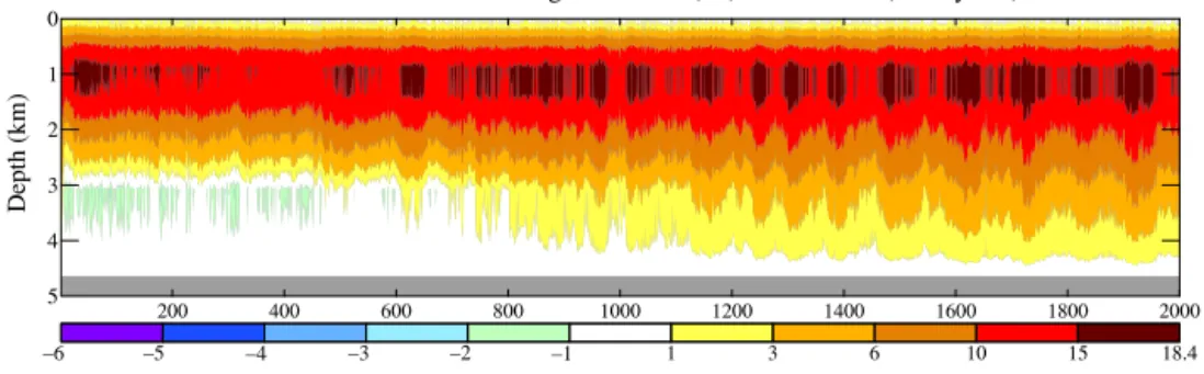
Atlantic meridional overturning circulation (Sv): Control run (2000 years)
–6 –5 –4 –3 –2 –1
Figure 3. Annual mean AMOC (Sv) at 28◦N in the model control run.
Figure 4. Climate response function, R(t), i.e., the fraction (%) of
equilibrium surface temperature response for GISS modelE-R based on a 2000-year control run (Hansen et al., 2007a). Forcing was in-stant CO2doubling with fixed ice sheets, vegetation distribution,
and other long-lived GHGs.
less computing time using the 5-, 10- and 20-year doubling times. Observed ice sheet mass loss doubling rates, although records are short, are ∼ 10 years (Sect. 5.1). Our sharp cut-off of melt aids separation of immediate forcing effects and feedbacks.
We argue that such a rapid increase in meltwater is plausi-ble if GHGs keep growing rapidly. Greenland and Antarctica have outlet glaciers in canyons with bedrock below sea level well back into the ice sheet (Fretwell et al., 2013; Morlighem et al., 2014; Pollard et al., 2015). Feedbacks, including ice sheet darkening due to surface melt (Hansen et al., 2007b; Robinson et al., 2012; Tedesco et al., 2013; Box et al., 2012) and lowering and thus warming of the near-coastal ice sheet surface, make increasing ice melt likely. Paleoclimate data reveal sea level rise of several meters in a century (Fair-banks, 1989; Deschamps et al., 2012). Those cases involved ice sheets at lower latitudes, but 21st century climate forcing is larger and increasing much more rapidly.
Radiative forcings (Fig. S16a, b) are from Hansen et al. (2007c) through 2003 and IPCC scenario A1B for later GHGs. A1B is an intermediate IPCC scenario over the cen-tury, but on the high side early this century (Fig. 2 of Hansen et al., 2007c). We add freshwater to the North Atlantic (ocean area within 52–72◦N and 15◦E–65◦N) or Southern Ocean (ocean south of 60◦ S), or equally divided between the two oceans. Ice sheet discharge (icebergs plus meltwater) is mixed as freshwater with mean temperature −15◦C into the top three ocean layers (Fig. S6).
3.4 Simulated surface temperature and energy balance We present surface temperature and planetary energy balance first, thus providing a global overview. Then we examine changes in ocean circulation and compare results with prior studies.
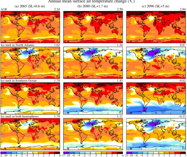
Temperature change in 2065, 2080 and 2096 for 10-year doubling time (Fig. 6) should be thought of as results when sea level rise reaches 0.6, 1.7 and 5 m, because the dates de-pend on initial freshwater flux. Actual current freshwater flux may be about a factor of 4 higher than assumed in these initial runs, as we will discuss, and thus effects may occur ∼20 years earlier. A sea level rise of 5 m in a century is about the most extreme in the paleo-record (Fairbanks, 1989; De-schamps et al., 2012), but the assumed 21st century climate forcing is also more rapidly growing than any known natural forcing.
Meltwater injected into the North Atlantic has larger ini-tial impact, but Southern Hemisphere ice melt has a greater global effect for larger melt as the effectiveness of more melt-water in the North Atlantic begins to decline. The global ef-fect is large long before sea level rise of 5 m is reached. Melt-water reduces global warming about half by the time sea level rise reaches 1.7 m. Cooling due to ice melt more than elimi-nates A1B warming in large areas of the globe.
The large cooling effect of ice melt does not decrease much as the ice melting rate varies between doubling times of 5, 10 or 20 years (Fig. 7a). In other words, the cumulative ice sheet melt, rather than the rate of ice melt, largely deter-mines the climate impact for the range of melt rates covered by 5-, 10- and 20-year doubling times. Thus if ice sheet loss
Figure 5. (a) Total freshwater flux added in the North Atlantic and Southern oceans and (b) resulting sea level rise. Solid lines for 1 m sea
level rise, dotted for 5 m. One sverdrup (Sv) is 106m3s−1, which is ∼ 3× 10⁴Gt year−1.
Annual mean surface air temperature change ( C)
Ice melt in North Atlantic
Ice melt in Southern Ocean
Ice melt in both hemispheres
–12 –10 –6 –4 –2 –1 –17–10 –6 –4 –2 –1 –21–10 –6 –4 –2 –1
–0.33 –0.02
Figure 6. Surface air temperature (◦C) relative to 1880–1920 in (a) 2065, (b) 2080, and (c) 2096. Top row is IPCC scenario A1B. Ice melt with 10-year doubling is added in other scenarios.
occurs even to an extent of 1.7 m sea level rise (Fig. 7b), a large impact on climate and climate change is predicted.
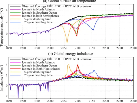
Greater global cooling occurs for freshwater injected into the Southern Ocean, but the cooling lasts much longer for North Atlantic injection (Fig. 7a). That persistent cooling, mainly at Northern Hemisphere middle and high latitudes
(Fig. S7), is a consequence of the sensitivity, hysteresis ef-fects, and long recovery time of the AMOC (Stocker and Wright, 1991; Rahmstorf, 1995, and earlier studies refer-enced therein). AMOC changes are described below.
When freshwater injection in the Southern Ocean is halted, global temperature jumps back within two decades to the
Figure 7. (a) Surface air temperature (◦C) relative to 1880–1920 for several scenarios. (b) Global energy imbalance (W m−2)for the same scenarios.
value it would have had without any freshwater addition (Fig. 7a). Quick recovery is consistent with the Southern Ocean-centric picture of the global overturning circulation (Fig. 4; Talley, 2013), as the Southern Ocean meridional overturning circulation (SMOC), driven by AABW forma-tion, responds to change in the vertical stability of the ocean column near Antarctica (Sect. 3.7) and the ocean mixed layer and sea ice have limited thermal inertia.
Cooling from ice melt is largely regional, temporary, and does not alleviate concerns about global warming. Southern Hemisphere cooling is mainly in uninhabited regions. North-ern Hemisphere cooling increases temperature gradients that will drive stronger storms (Sect. 3.9).
Global cooling due to ice melt causes a large increase in Earth’s energy imbalance (Fig. 7b), adding about +2 W m−2, which is larger than the imbalance caused by increasing GHGs. Thus, although the cold freshwater from ice sheet disintegration provides a negative feedback on regional and global surface temperature, it increases the planet’s energy imbalance, thus providing more energy for ice melt (Hansen, 2005). This added energy is pumped into the ocean.
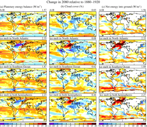
Increased downward energy flux at the top of the atmo-sphere is not located in the regions cooled by ice melt. How-ever, those regions suffer a large reduction of net incoming energy (Fig. 8a). The regional energy reduction is a conse-quence of increased cloud cover (Fig. 8b) in response to the colder ocean surface. However, the colder ocean surface re-duces upward radiative, sensible and latent heat fluxes, thus causing a large (∼ 50 W m−2) increase in energy into the
North Atlantic and a substantial but smaller flux into the Southern Ocean (Fig. 8c).
Below we conclude that the principal mechanism by which this ocean heat increases ice melt is via its effect on ice shelves. Discussion requires examination of how the fresh-water injections alter the ocean circulation and internal ocean temperature.
3.5 Simulated Atlantic meridional overturning circulation (AMOC)
Broecker’s articulation of likely effects of freshwater out-bursts in the North Atlantic on ocean circulation and global climate (Broecker, 1990; Broecker et al., 1990) spurred quan-titative studies with idealized ocean models (Stocker and Wright, 1991) and global atmosphere–ocean models (Man-abe and Stouffer, 1995; Rahmstorf 1995, 1996). Scores of modeling studies have since been carried out, many reviewed by Barreiro et al. (2008), and observing systems are being developed to monitor modern changes in the AMOC (Carton and Hakkinen, 2011).
Our climate simulations in this section are five-member ensembles of runs initiated at 25-year intervals at years 901– 1001 of the control run. We chose this part of the control run because the planet is then in energy balance (Fig. S1), although by that time model drift had altered the slow deep-ocean circulation. Some model drift away from initial clima-tological conditions is inevitable, as all models are imperfect, and we carry out the experiments with cognizance of model limitations. However, there is strong incentive to seek basic
Change in 2080 relative to 1880–1920
(a) Planetary energy balance (W/m ) (b) Cloud cover (%) (c) Net energy into ground (W/m )
Ice melt in North Atlantic Ice melt in North Atlantic Ice melt in North Atlantic
Ice melt in Southern Ocean Ice melt in Southern Ocean Ice melt in Southern Ocean
Ice melt in both hemispheres Ice melt in both hemispheres Ice melt in both hemispheres
–20 –15 –10 –6 –3 –1 –22–10 –6 –3 –1 –.5 –74–50 –20 –10 –5 –2
Figure 8. Change in 2080 (mean of 2078–2082), relative to 1880–1920, of annual mean (a) planetary energy balance (W m−2), (b) cloud cover (%), and (c) net energy into ground (W m−2)for the same scenarios as Fig. 6.
improvements in representation of physical processes to re-duce drift in future versions of the model.
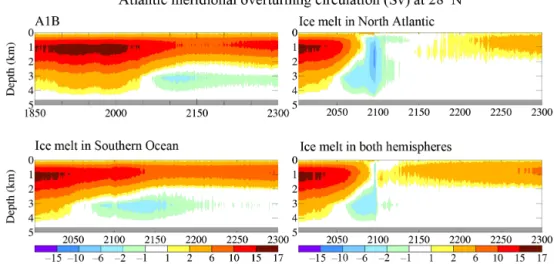
GHGs alone (scenario A1B) slow AMOC by the early 21st century (Fig. 9), but variability among individual runs (Fig. S8) would make definitive detection difficult at present. Freshwater injected into the North Atlantic or in both hemi-spheres shuts down the AMOC (Fig. 9, right side). GHG amounts are fixed after 2100 and ice melt is zero, but after two centuries of stable climate forcing the AMOC has not recovered to its earlier state. This slow recovery was found in the earliest simulations by Manabe and Stouffer (1994) and Rahmstorf (1995, 1996).
Freshwater injection already has a large impact when ice melt is a fraction of 1 m of sea level. By the time sea level rise reaches 59 cm (2065 in the present scenarios), when fresh-water flux is 0.48 Sv, the impact on AMOC is already large, consistent with the substantial surface cooling in the North Atlantic (Fig. 6).
3.6 Comparison with prior simulations
AMOC sensitivity to GHG forcing has been examined ex-tensively based on CMIP studies. Schmittner et al. (2005) found that AMOC weakened 25 ± 25 % by the end of the 21st century in 28 simulations of 9 different models forced by the A1B emission scenario. Gregory et al. (2005) found 10– 50 % AMOC weakening in 11 models for CO2quadrupling
(1 % year−1increase for 140 years), with largest decreases in models with strong AMOCs. Weaver et al. (2007) found a 15–31 % AMOC weakening for CO2quadrupling in a single
model for 17 climate states differing in initial GHG amount. AMOC in our model weakens 30 % in the century between 1990–2000 and 2090–2100, the period used by Schmittner et al. (2005), for A1B forcing (Fig. S8). Thus our model is more sensitive than the average but within the range of other models, a conclusion that continues to be valid in comparison with 10 CMIP5 models (Cheng et al., 2013).
AMOC sensitivity to freshwater forcing has not been com-pared as systematically among models. Several studies find little impact of Greenland melt on AMOC (Huybrechts et
Figure 9. Ensemble-mean AMOC (Sv) at 28◦N versus time for the same four scenarios as in Fig. 6, with ice melt reaching 5 m at the end of the 21st century in the three experiments with ice melt.
al., 2002; Jungclaus et al., 2006; Vizcaino et al., 2008) while others find substantial North Atlantic cooling (Fichefet et al., 2003; Swingedouw et al., 2007; Hu et al., 2009, 2011). Stud-ies with little impact calculated or assumed small ice sheet melt rates, e.g., Greenland contributed only 4 cm of sea level rise in the 21st century in the ice sheet model of Huybrechts et al. (2002). Fichefet et al. (2003), using nearly the same atmosphere–ocean model as Huybrechts et al. (2002) but a more responsive ice sheet model, found AMOC weakening from 20 to 13 Sv late in the 21st century, but separate contri-butions of ice melt and GHGs to AMOC slowdown were not defined.
Hu et al. (2009, 2011) use the A1B scenario and freshwa-ter from Greenland starting at 1 mm sea level per year in-creasing 7 % year−1, similar to our 10-year doubling case. Hu et al. keep the melt rate constant after it reaches 0.3 Sv (in 2050), yielding 1.65 m sea level rise in 2100 and 4.2 m in 2200. Global warming found by Hu et al. for scenario A1B resembles our result but is 20–30 % smaller (compare Fig. 2b of Hu et al., 2009 to our Fig. 6), and cooling they obtain from the freshwater flux is moderately less than that in our model. AMOC is slowed about one-third by the latter 21st century in the Hu et al. (2011) 7 % year−1experiment, comparable to our result.
General consistency holds for other quantities, such as changes of precipitation. Our model yields southward shift-ing of the Intertropical Convergence Zone (ITCZ) and in-tensification of the subtropical dry region with increasing GHGs (Fig. S9), as has been reported in modeling studies of Swingedouw et al. (2007, 2009). These effects are inten-sified by ice melt and cooling in the North Atlantic region (Fig. S9).
A recent five-model study (Swingedouw et al., 2014) finds a small effect on AMOC for 0.1 Sv Greenland freshwater flux added in 2050 to simulations with a strong GHG forcing. Our
larger response is likely due, at least in part, to our freshwater flux reaching several tenths of a sverdrup.
3.7 Pure freshwater experiments
We assumed, in discussing the relevance of these experi-ments to Eemian climate, that effects of freshwater injec-tion dominate over changing GHG amount, as seems likely because of the large freshwater effect on sea surface tem-peratures (SSTs) and sea level pressure. However, Eemian CO2was actually almost constant at ∼ 275 ppm (Luthi et al.,
2008). Thus, to isolate effects better, we now carry out sim-ulations with fixed GHG amount, which helps clarify impor-tant feedback processes.
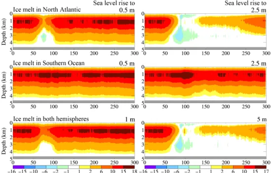
Our pure freshwater experiments are five-member ensem-bles starting at years 1001, 1101, 1201, 1301, and 1401 of the control run. Each experiment ran 300 years. Freshwater flux in the initial decade averaged 180 km3year−1 (0.5 mm sea level) in the hemisphere with ice melt and increased with a 10-year doubling time. Freshwater input is terminated when it reaches 0.5 m sea level rise per hemisphere for three five-member ensembles: two ensembles with injection in the in-dividual hemispheres and one ensemble with input in both hemispheres (1 m total sea level rise). Three additional en-sembles were obtained by continuing freshwater injection until hemispheric sea level contributions reached 2.5 m. Here we provide a few model diagnostics central to discussions that follow. Additional results are provided in Figs. S10–S12. The AMOC shuts down for Northern Hemisphere fresh-water input yielding 2.5 m sea level rise (Fig. 10). By year 300, more than 200 years after cessation of all freshwater in-put, AMOC is still far from full recovery for this large fresh-water input. On the other hand, freshfresh-water input of 0.5 m does not cause full shutdown, and AMOC recovery occurs in less than a century.
Figure 10. Ensemble-mean AMOC (Sv) at 28◦N versus time for six pure freshwater forcing experiments.
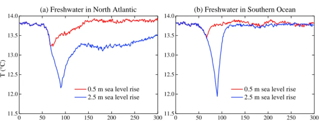
Global temperature change (Fig. 11) reflects the funda-mentally different impact of freshwater forcings of 0.5 and 2.5 m. The response also differs greatly depending on the hemisphere of the freshwater input. The case with freshwater forcing in both hemispheres is shown only in the Supplement because, to a good approximation, the response is simply the sum of the responses to the individual hemispheric forcings (see Figs. S10–S12). The sum of responses to hemispheric forcings moderately exceeds the response to global forcing.
Global cooling continues for centuries for the case with freshwater forcing sufficient to shut down the AMOC (Fig. 11). If the forcing is only 0.5 m of sea level, the tem-perature recovers in a few decades. However, the freshwater forcing required to reach the tipping point of AMOC shut-down may be less in the real world than in our model, as discussed below. Global cooling due to freshwater input on the Southern Ocean disappears in a few years after freshwa-ter input ceases (Fig. 11), for both the smaller (0.5 m of sea level) and larger (2.5 m) freshwater forcings.
Injection of a large amount of surface freshwater in ei-ther hemisphere has a notable impact on heat uptake by the ocean and the internal ocean heat distribution (Fig. 12). De-spite continuous injection of a large amount of very cold (−15◦C) water in these pure freshwater experiments, sub-stantial portions of the ocean interior become warmer. Trop-ical and Southern Hemisphere warming is the well-known effect of reduced heat transport to northern latitudes in re-sponse to the AMOC shutdown (Rahmstorf, 1996; Barreiro et al., 2008).
However, deep warming in the Southern Ocean may have greater consequences. Warming is maximum at grounding line depths (∼ 1–2 km) of Antarctic ice shelves (Rignot and Jacobs, 2002). Ice shelves near their grounding lines (Fig. 13 of Jenkins and Doake, 1991) are sensitive to temperature of the proximate ocean, with ice shelf melting increasing 1 m per year for each 0.1◦C temperature increase (Rignot and Ja-cobs, 2002). The foot of an ice shelf provides most of the re-straining force that ice shelves exert on landward ice (Fig. 14 of Jenkins and Doake, 1991), making ice near the grounding line the buttress of the buttress. Pritchard et al. (2012) deduce from satellite altimetry that ice shelf melt has primary control of Antarctic ice sheet mass loss.
Thus we examine our simulations in more detail (Fig. 13). The pure freshwater experiments add 5 mm sea level in the first decade (requiring an initial 0.346 mm year−1for 10-year doubling), 10 mm in the second decade, and so on (Fig. 13a). Cumulative freshwater injection reaches 0.5 m in year 68 and 2.5 m in year 90.
Antarctic Bottom Water (AABW) formation is reduced ∼20 % by year 68 and ∼ 50 % by year 90 (Fig. 13b). When freshwater injection ceases, AABW formation rapidly re-gains full strength, in contrast to the long delay in reestab-lishing North Atlantic Deep Water (NADW) formation af-ter AMOC shutdown. The Southern Ocean mixed-layer re-sponse time dictates the recovery time for AABW forma-tion. Thus rapid recovery also applies to ocean temperature at depths of ice shelf grounding lines (Fig. 13c). The rapid response of the Southern Ocean meridional overturning
cir-0 50 100 150 200 250 300 11.5 12.0 12.5 13.0 13.5 14.0
0.5 m sea level rise 2.5 m sea level rise (a) Freshwater in North Atlantic
T (
°
C)
Global surface air temperature
0 50 100 150 200 250 300 11.5 12.0 12.5 13.0 13.5 14.0
0.5 m sea level rise 2.5 m sea level rise (b) Freshwater in Southern Ocean
Figure 11. Ensemble-mean global surface air temperature (◦C) for experiments (years on x axis) with freshwater forcing in either the North Atlantic Ocean (left) or the Southern Ocean (right).
Ocean temperature change ( C) in pure freshwater experiment
Freshwater in both hemispheres, SL rise = 5 m Freshwater in Southern Ocean, SL rise = 2.5 m Freshwater in North Atlantic, SL rise = 2.5 m
Figure 12. Change of ocean temperature (◦C) relative to control run due to freshwater input that reaches 2.5 m of global sea level in a hemisphere (thus 5 m sea level rise in the bottom row).
culation (SMOC) implies that the rate of freshwater addition to the mixed layer is the driving factor.
Freshwater flux has little effect on simulated Northern Hemisphere sea ice until the 7th decade of freshwater growth (Fig. 13d), but Southern Hemisphere sea ice is more sensi-tive, with substantial response in the 5th decade and large re-sponse in the 6th decade. Below we show that “5th decade” freshwater flux (2880 Gt year−1) is already relevant to the
Southern Ocean today.
3.8 Simulations to 2100 with modified (more realistic) forcings
Recent data show that current ice melt is larger than assumed in our 1850–2300 simulations. Thus we make one more sim-ulation and include minor improvements in the radiative forc-ing.
3.8.1 Advanced (earlier) freshwater injection
Atmosphere–ocean climate models, including ours, com-monly include a fixed freshwater flux from the Greenland and Antarctic ice sheets to the ocean. This flux is chosen to balance snow accumulation in the model’s control run, with
0 50 100 150 200 250 300 0
1 10 100
0.5 m sea level rise 2.5 m sea level rise (a) Rate of freshwater input
Flux (Tt/year) 0 50 100 150 200 250 300 −7 −6 −5 −4 −3 −2
0.5 m sea level rise 2.5 m sea level rise (b) SMOC (mean ocean overturning at 72°S)
SMOC (Sv) 0 50 100 150 200 250 300 −1.4 −1.2 −1.0 −.8
−.6 0.5 m sea level rise
2.5 m sea level rise (c) Ocean temperature at ~1 km depth at 74°S
T ( ° C) 0 50 100 150 200 250 300 0 2 4 6 8 10 12
(d) Sea ice cover in hemisphere of FW input
Ice cover (%)
Southern Hemisphere Northern Hemisphere
Figure 13. (a) Freshwater input (Tt year−1) to Southern Ocean (1 Tt = 1000 km3). (b, c, d) Simulated overturning strength (Sv) of AABW cell at 72◦S, temperature (◦C) at depth 1.13 km at 74◦S, and sea ice cover (%).
the rationale that approximate balance is expected between net accumulation and mass loss including icebergs and ice shelf melting. Global warming creates a mass imbalance that we want to investigate. Ice sheet models can calculate the im-balance, but it is unclear how reliably ice sheet models sim-ulate ice sheet disintegration. We forgo ice sheet modeling, instead adding a growing freshwater amount to polar oceans with alternative growth rates and initial freshwater amount estimated from available data.
Change of freshwater flux into the ocean in a warming world with shrinking ice sheets consists of two terms: term 1 being net ice melt and term 2 being change in P − E (pre-cipitation minus evaporation) over the relevant ocean. Term 1 includes land based ice mass loss, which can be detected by satellite gravity measurements, loss of ice shelves, and net sea ice mass change. Term 2 is calculated in a climate model forced by changing atmospheric composition, but it is not included in our pure freshwater experiments that have no global warming.
IPCC (Vaughan et al., 2013) estimated land ice loss in Antarctica that increased from 30 Gt year−1 in 1992–2001 to 147 Gt year−1 in 2002–2011 and in Greenland from 34 to 215 Gt year−1, with uncertainties discussed by Vaughan et al. (2013). Gravity satellite data suggest Greenland ice sheet mass loss ∼ 300–400 Gt year−1 in the past few years (Barletta et al., 2013). A newer analysis of gravity data for 2003–2013 (Velicogna et al., 2014), discussed in more detail in Sect. 5.1, finds a Greenland mass loss 280 ± 58 Gt year−1
and Antarctic mass loss 67 ± 44 Gt year−1.
One estimate of net ice loss from Antarctica, including ice shelves, is obtained by surveying and adding the mass flux from all ice shelves and comparing this freshwater mass loss with the freshwater mass gain from the continental sur-face mass budget. Rignot et al. (2013) and Depoorter et al. (2013) independently assessed the freshwater mass fluxes from Antarctic ice shelves. Their respective estimates for the basal melt are 1500 ± 237 and 1454 ± 174 Gt year−1.
Their respective estimates for calving are 1265 ± 139 and 1321 ± 144 Gt year−1.
This estimated freshwater loss via the ice shelves (∼ 2800 Gt year−1) is larger than freshwater gain by Antarc-tica. Vaughan et al. (1999) estimated net surface mass bal-ance of the continent as +1811 and +2288 Gt year−1 in-cluding precipitation on ice shelves. Vaughan et al. (2013) estimates the net Antarctic surface mass balance as +1983 ± 122 Gt year−1excluding ice shelves. Thus compar-ison of continental freshwater input with ice shelf output sug-gests a net export of freshwater to the Southern Ocean of sev-eral hundred Gt year−1in recent years. However, substantial
uncertainty exists in the difference between these two large numbers.
An independent evaluation has recently been achieved by Rye et al. (2014) using satellite measured changes of sea level around Antarctica in the period 1992–2011. Sea level along the Antarctic coast rose 2 mm year−1 faster than the regional mean sea level rise in the Southern Ocean south of 50◦S, an effect that they conclude is almost entirely a steric adjustment caused by accelerating freshwater discharge from Antarctica. They conclude that an excess freshwater input of 430 ± 230 Gt year−1, above the rate needed to maintain a steady ocean salinity, is required. Rye et al. (2014) note that these values constitute a lower bound for the actual excess discharge above a “steady salinity” rate, because numerous in situ data, discussed below, indicate that freshening began earlier than 1992.
Term 2, change in P − E over the Southern Ocean rela-tive to its preindustrial amount, is large in our climate sim-ulations. In our ensemble of runs (using observed GHGs for 1850–2003 and scenario A1B thereafter) the increase in P − Ein the decade 2011–2020, relative to the control run, was in the range 3500 to 4000 Gt year−1, as mean precipita-tion over the Southern Ocean increased ∼ 35 mm year−1and evaporation decreased ∼ 3 mm year−1.
Increasing ice melt and increasing P − E are climate feed-backs, their growth in recent decades driven by global
warm-ing. Our pure freshwater simulations indicate that their sum, at least 4000 Gt year−1, is sufficient to affect ocean
circula-tion, sea ice cover, and surface temperature, which can spur other climate feedbacks. We investigate these feedbacks via climate simulations using improved estimates of freshwater flux from ice melt. P − E is computed by the model.
We take freshwater injection to be 720 Gt year−1 from Antarctica and 360 Gt year−1in the North Atlantic in 2011, with injection rates at earlier and later times defined by assumption of a 10-year doubling time. Resulting mean freshwater injection around Antarctica in 1992–2011 is ∼400 Gt year−1, similar to the estimate of Rye et al. (2014). A recent estimate of 310 ± 74 km3 volume loss of floating Antarctic ice shelves in 2003–2012 (Paolo et al., 2015) is not inconsistent, as the radar altimeter data employed for ice shelves do not include contributions from the ice sheet or fast ice tongues at the ice shelf grounding line. Greenland ice sheet mass loss provides most of the assumed 360 Gt year−1
freshwater, and this would be supplemented by shrinking ice shelves (Rignot and Steffen, 2008) and small ice caps in the North Atlantic and west of Greenland (Ohmura, 2009) that are losing mass (Abdalati et al., 2004; Bahr et al., 2009).
We add freshwater around Antarctica at coastal grid boxes (Fig. S13) guided by the data of Rignot et al. (2013) and De-poorter et al. (2013). Injection in the Western Hemisphere, especially from the Weddell Sea to the Ross Sea, is more than twice that in the other hemisphere (Fig. 14). Specified freshwater flux around Greenland is similar on the east and west coasts, and small along the north coast (Fig. S13). 3.8.2 Modified radiative forcings
Actual GHG forcing is less than scenario A1B, because CH4
and minor gas growth declined after IPCC scenarios were defined (Fig. 5; Hansen et al., 2013c, update at http://www. columbia.edu/~mhs119/GHGs/). As a simple improvement we decreased the A1B CH4 scenario during 2003–2013 so
that subsequent CH4is reduced 100 ppb, decreasing radiative
forcing ∼ 0.05 W m−2.
Stratospheric aerosol forcing to 2014 uses the data set of Sato et al. (1993) as updated at http://www.columbia.edu/ ~mhs119/StratAer/. Future years have constant aerosol op-tical depth 0.0052 yielding effective forcing −0.12 W m−2, implemented by using fixed 1997 aerosol data. Tropospheric aerosol growth is assumed to slow smoothly, leveling out at −2 W m−2in 2100. Future solar forcing is assumed to have
an 11-year cycle with amplitude 0.25 W m−2. Net forcing
ex-ceeds 5 W m−2by the end of the 21st century, about 3 times
the current forcing (Fig. S16).
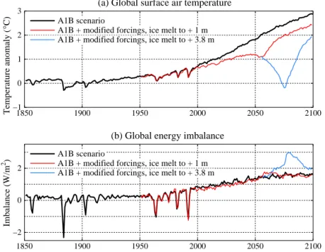
3.8.3 Climate simulations with modified forcings Global temperature has a maximum at +1.2◦C in the 2040s for the modified forcings (Fig. 15). Ice melt cooling is ad-vanced as global ice melt reaches 1 m of sea level in 2060,
−180 −150 −120 −90 −60 −30 0 30 60 90 120 150 180 0 50 100 150 200 250 Calving Basal melt Freshwater production by calving and basal melt
Longitude (°)
Ice flux (Gt/yr)
Figure 14. Freshwater flux (Gt year−1) from Antarctic ice shelves based on data of Rignot et al. (2013), integrated here into intervals of 15◦ of longitude. Depoorter et al. (2013) data yield a similar distribution.
1/3 from Greenland and 2/3 from Antarctica. Global tem-perature rise resumes in the 2060s after cessation of freshwa-ter injection.
Global temperature becomes an unreliable diagnostic of planetary condition as the ice melt rate increases. Global en-ergy imbalance (Fig. 15b) is a more meaningful measure of planetary status as well as an estimate of the climate forcing change required to stabilize climate. Our calculated present energy imbalance of ∼ 0.8 W m−2 (Fig. 15b) is larger than the observed 0.58 ± 0.15 W m−2during 2005–2010 (Hansen et al., 2011). The discrepancy is likely accounted for by ex-cessive ocean heat uptake at low latitudes in our model, a problem related to the model’s slow surface response time (Fig. 4) that may be caused by excessive small-scale ocean mixing.
Large scale regional cooling occurs in the North Atlantic and Southern oceans by mid-century (Fig. 16) for 10-year doubling of freshwater injection. A 20-year doubling places similar cooling near the end of this century, 40 years ear-lier than in our prior simulations (Fig. 7), as the factor of 4 increase in current freshwater from Antarctica is a 40-year advance.
Cumulative North Atlantic freshwater forcing in sverdrup years (Sv years) is 0.2 Sv years in 2014, 2.4 Sv years in 2050, and 3.4 Sv years (its maximum) prior to 2060 (Fig. S14). The critical issue is whether human-spurred ice sheet mass loss can be approximated as an exponential process during the next few decades. Such nonlinear behavior depends upon amplifying feedbacks, which, indeed, our climate simula-tions reveal in the Southern Ocean.
3.8.4 Southern Ocean feedbacks
Amplifying feedbacks in the Southern Ocean and atmo-sphere contribute to dramatic climate change in our simula-tions (Fig. 16). We first summarize the feedbacks to identify processes that must be simulated well to draw valid conclu-sions. While recognizing the complexity of the global ocean circulation (Lozier, 2012; Lumpkin and Speer, 2007; Mar-shall and Speer, 2012; Munk and Wunsch, 1998; Orsi et al., 1999; Sheen et al., 2014; Talley, 2013; Wunsch and Ferrari,
1850 1900 1950 2000 2050 2100 −1 0 1 2 3 A1B scenario
A1B + modified forcings, ice melt to + 1 m A1B + modified forcings, ice melt to + 3.8 m
(a) Global surface air temperature
T em p er at u re an o m al y ( ° C ) 1850 1900 1950 2000 2050 2100 −2 0 2 A1B scenario
A1B + modified forcings, ice melt to + 1 m A1B + modified forcings, ice melt to + 3.8 m
(b) Global energy imbalance
Imbalance (W/m
2)
Figure 15. (a) Surface air temperature (◦C) change relative to 1880–1920 and (b) global energy imbalance (W m−2)for the modified forcing scenario including cases with global ice melt reaching 1 and 3.8 m.
2055–2060 surface air temperature ( C) relative to 1880–1920 A1B + modified forcings, ice melt to 1 m
Figure 16. Surface air temperature (◦C) change relative to 1880– 1920 in 2055–2060 for modified forcings.
2004), we use a simple two-dimensional representation to discuss the feedbacks.
Climate change includes slowdown of AABW formation, indeed shutdown by mid-century if freshwater injection in-creases with a doubling time as short as 10 years (Fig. 17). Implications of AABW shutdown are so great that we must ask whether the mechanisms are simulated with sufficient re-alism in our climate model, which has coarse resolution and relevant deficiencies that we have noted. After discussing the feedbacks here, we examine how well the processes are in-cluded in our model (Sect. 3.8.5). Paleoclimate data (Sect. 4)
provide much insight about these processes, and modern ob-servations (Sect. 5) suggest that these feedbacks are already underway.
Large-scale climate processes affecting ice sheets are sketched in Fig. 18. The role of the ocean circulation in the global energy and carbon cycles is captured to a useful extent by the two-dimensional (zonal-mean) overturning circulation featuring deep water (NADW) and bottom water (AABW) formation in the polar regions. Marshall and Speer (2012) discuss the circulation based in part on tracer data and analy-ses by Lumpkin and Speer (2007). Talley (2013) extends the discussion with diagrams clarifying the role of the Pacific and Indian oceans.
Wunsch (2002) emphasizes that the ocean circulation is driven primarily by atmospheric winds and secondarily by tidal stirring. Strong circumpolar westerly winds provide en-ergy drawing deep water toward the surface in the South-ern Ocean. Ocean circulation also depends on processes maintaining the ocean’s vertical density stratification. Winter cooling of the North Atlantic surface produces water dense enough to sink (Fig. 18), forming North Atlantic Deep Wa-ter (NADW). However, because North Atlantic waWa-ter is rel-atively fresh, compared to the average ocean, NADW does not sink all the way to the global ocean bottom. Bottom water is formed instead in the winter around the Antarctic coast, where very salty cold water (AABW) can sink to the ocean floor. This ocean circulation (Fig. 18) is altered by nat-ural and human-made forcings, including freshwater from ice sheets, engendering powerful feedback processes.
Global meridional overturning circulation (Sv) at 72 S A1b + Modified forcings, ice melt to 1 m
Figure 17. SMOC, ocean overturning strength (Sv) at 72◦S, including only the mean (Eulerian) transport. This is the average of a five-member model ensemble for the modified forcing including advanced ice melt (720 Gt year−1from Antarctica in 2011) and 10-year doubling.
Figure 18. Schematic of stratification and precipitation amplifying feedbacks. Stratification: increased freshwater flux reduces surface water
density, thus reducing AABW formation, trapping NADW heat, and increasing ice shelf melt. Precipitation: increased freshwater flux cools ocean mixed layer, increases sea ice area, causing precipitation to fall before it reaches Antarctica, reducing ice sheet growth and increasing ocean surface freshening. Ice in West Antarctica and the Wilkes Basin, East Antarctica, is most vulnerable because of the instability of retrograde beds.
A key Southern Ocean feedback is meltwater stratification effect, which reduces ventilation of ocean heat to the atmo-sphere and space. Our “pure freshwater” experiments show that the low-density lid causes deep-ocean warming, espe-cially at depths of ice shelf grounding lines that provide most of the restraining force limiting ice sheet discharge (Fig. 14 of Jenkins and Doake, 1991). West Antarctica and Wilkes Basin in East Antarctica have potential to cause rapid sea level rise, because much of their ice sits on retrograde beds (beds sloping inland), a situation that can lead to unstable grounding line retreat and ice sheet disintegration (Mercer, 1978).
Another feedback occurs via the effect of surface and atmospheric cooling on precipitation and evaporation over the Southern Ocean. CMIP5 climate simulations, which do
not include increasing freshwater injection in the Southern Ocean, find snowfall increases on Antarctica in the 21st cen-tury, thus providing a negative term to sea level change. Frieler et al. (2015) note that 35 climate models are consis-tent in showing that warming climate yields increasing snow accumulation in accord with paleo-data for warmer climates, but the paleo-data refer to slowly changing climate in quasi-equilibrium with ocean boundary conditions. In our experi-ments with growing freshwater injection, the increasing sea ice cover and cooling of the Southern Ocean surface and at-mosphere cause the increased precipitation to occur over the Southern Ocean, rather than over Antarctica. This feedback not only reduces any increase in snowfall over Antarctica but also provides a large freshening term to the surface of the
Maximum winter mixed layer depth (km) Maximum winter mixed layer depth (%)
Figure 19. Maximum mixed-layer depth (in km, left, and % of ocean depth, right) in February (Northern Hemisphere) and August (Southern
Hemisphere) using the mixed-layer definition of Heuze et al. (2013).
Southern Ocean, thus magnifying the direct freshening effect from increasing ice sheet melt.
North Atlantic meltwater stratification effects are also im-portant, but different. Meltwater from Greenland can slow or shutdown NADW formation, cooling the North Atlantic, with global impacts even in the Southern Ocean, as we will discuss later. One important difference is that the North At-lantic can take centuries to recover from NADW shutdown, while the Southern Ocean recovers within 1–2 decades after freshwater injection stops (Sect. 3.7).
3.8.5 Model’s ability to simulate these feedbacks Realistic representation of these feedbacks places require-ments on both the atmosphere and ocean components of our climate model. We discuss first the atmosphere, then the ocean.
There are two main requirements on the atmospheric model. First, it must simulate P − E well, because of its im-portance for ocean circulation and the amplifying feedback in the Southern Ocean. Second, it must simulate winds well, because these drive the ocean.
Simulated P −E (Fig. S15b) agrees well with meteorolog-ical reanalysis (Fig. 3.4b of Rhein et al., 2013). Resulting sea surface salinity (SSS) patterns in the model (Fig. S15a) agree well with global ocean surface salinity patterns (Antonov et al., 2010, and Fig. 3.4a of Rhein et al., 2013). SSS trends in our simulation (Fig. S15c), with the Pacific on average be-coming fresher while most of the Atlantic and the subtropics in the Southern Hemisphere become saltier, are consistent with observed salinity trends (Durack and Wijffels, 2010). Recent freshening of the Southern Ocean in our simulation is somewhat less than in observed data (Fig. 3.4c, d of Rhein et al., 2013), implying that the amplifying feedback may be underestimated in our simulation. A likely reason for that is discussed below in conjunction with observed sea ice change. Obtaining accurate winds requires the model to simulate well atmospheric pressure patterns and their change in
re-sponse to climate forcings. A test is provided by observed changes of the Southern Annular Mode (SAM), with a de-crease in surface pressure near Antarctica and a small in-crease at midlatitudes (Marshall, 2003) that Thompson et al. (2011) relate to stratospheric ozone loss and increasing GHGs. Our climate forcing (Fig. S16) includes ozone change (Fig. 2 of Hansen et al., 2007a) with stratospheric ozone depletion in 1979–1997 and constant ozone thereafter. Our model produces a trend toward the high index polarity of SAM (Fig. S17) similar to observations, although perhaps a slightly smaller change than observed (compare Fig. S17 with Fig. 3 of Marshall, 2003). SAM continues to increase in our model after ozone stabilizes (Fig. S17), suggesting that GHGs may provide a larger portion of the SAM re-sponse in our model than in the model study of Thompson et al. (2011). It would not be surprising if the stratospheric dy-namical response to ozone change were weak in our model, given the coarse resolution and simplified representation of atmospheric drag and dynamical effects in the stratosphere (Hansen et al., 2007a), but that is not a major concern for our present purposes.
The ocean model must be able to simulate realistically the ocean’s overturning circulation and its response to forcings including freshwater additions. Heuze et al. (2013, 2015) point out that simulated deep convection in the Southern Ocean is unrealistic in most models, with AABW formation occurring in the open ocean where it rarely occurs in nature. Our present ocean model contains significant improvements (see Sect. 3.2) compared to the GISS E2-R model that Heuze et al. include in their comparisons. Thus we show (Fig. 19) the maximum mixed-layer depth in winter (February in the Northern Hemisphere and August in the Southern Hemi-sphere) using the same criterion as Heuze et al. to define the mixed-layer depth, i.e., the layers with a density difference from the ocean surface layer less than 0.03 kg m−3.
Southern Ocean mixing in the model reaches a depth of ∼500 m in a wide belt near 60◦S stretching west from the southern tip of South America, with similar depths south
of Australia. These open-ocean mixed-layer depths compare favorably with observations shown in Fig. 2a of Heuze et al. (2015), based on data of de Boyer Montegut et al. (2004). There is no open-ocean deep convection in our model.
Deep convection occurs only along the coast of Antarc-tica (Fig. 19). Coastal grid boxes on the continental shelf are a realistic location for AABW formation. Orsi et al. (1999) suggest that most AABW is formed on shelves around the Weddell–Enderby Basin (60 %) and shelves of the Adélie– Wilkes Coast and Ross Sea (40 %). Our model produces mix-ing down to the shelf in those locations (Fig. 19b), and also on the Amery Ice Shelf near the location where Ohshima et al. (2013) identified AABW production, which they term Cape Darnley Bottom Water.
With our coarse 4◦stair step to the ocean bottom, AABW cannot readily slide down the slope to the ocean floor. Thus dense shelf water mixes into the open-ocean grid boxes, making our modeled Southern Ocean less stratified than the real world (cf. temporal drift of Southern Ocean salinity in Fig. S18), because the denser water must move several degrees of latitude horizontally before it can move deeper. Nevertheless, our Southern Ocean is sufficiently stratified to avoid the unrealistic open-ocean convection that infects many models (Heuze et al., 2013, 2015).
Orsi et al. (1999) estimate the AABW formation rate in several ways, obtaining values in the range 8–12 Sv, larger than our modeled 5–6 Sv (Fig. 17). However, as in most mod-els (Heuze et al., 2015), our SMOC diagnostic (Fig. 17) is the mean (Eulerian) circulation, i.e., excluding eddy-induced transport. Rerun of a 20-year segment of our control run to save eddy-induced changes reveals an increase in SMOC at 72◦S by 1–2 Sv, with negligible change at middle and low latitudes, making our simulated transport close to the range estimated by Orsi et al. (1999).
We conclude that the model may simulate Southern Ocean feedbacks that magnify the effect of freshwater injected into the Southern Ocean: the P − E feedback that wrings global-warming-enhanced water vapor from the air before it reaches Antarctica and the AABW slowdown that traps deep-ocean heat, leaving that heat at levels where it accelerates ice shelf melting. Indeed, we will argue that both of these feedbacks are probably underestimated in our current model.
The model seems less capable in Northern Hemisphere polar regions. Deep convection today is believed to occur mainly in the Greenland–Iceland–Norwegian (GIN) seas and at the southern end of Baffin Bay (Fig. 2b of Heuze et al., 2015). In our model, perhaps because of excessive sea ice in those regions, open-ocean deep convection occurs to the southeast of the southern tip of Greenland and at less deep grid boxes between that location and the United Kingdom (Fig. 19). Mixing reaching the ocean floor on the Siberian coast in our model (Fig. 19) may be realistic, as coastal polynya are observed on the Siberian continental shelf (D. Bauch et al., 2012). However, the winter mixed layer on the Alaska south coast is unrealistically deep (Fig. 19). These
model limitations must be kept in mind in interpreting simu-lated Northern Hemisphere climate change.
3.9 Impact of ice melt on storms
Our inferences about potential storm changes from continued high growth of atmospheric GHGs are fundamentally differ-ent than modeling results described in IPCC (2013, 2014), where the latter are based on CMIP5 climate model results without substantial ice sheet melt. Lehmann et al. (2014) note ambiguous results for storm changes from prior model stud-ies and describe implications of the CMIP5 ensemble of cou-pled climate models. Storm changes are moderate in nature, with even a weakening of storms in some locations and sea-sons. This is not surprising, because warming is greater at high latitudes, reducing meridional temperature gradients.
Before describing our model results, we note the model limitations for study of storms, including its coarse reso-lution (4◦×5◦), which may contribute to slight misplace-ment of the Bermuda high-pressure system for today’s cli-mate (Fig. S2). Excessive Northern Hemisphere sea ice may cause a bias in location of deepwater formation toward lower latitudes. Simulated effects also depend on the location cho-sen for freshwater injection; in model results shown here (Fig. 20), freshwater was spread uniformly over all longi-tudes in the North Atlantic between 65◦W and 15◦E. It would be useful to carry out similar studies with higher-resolution models including the most realistic possible dis-tribution of meltwater.
Despite these caveats, we have shown that the model real-istically simulates meridional changes of sea level pressure in response to climate forcings (Sect. 3.8.5). Specifically, the model yields a realistic trend to the positive phase of the Southern Annular Mode (SAM) in response to a decrease in stratospheric ozone and increase in other GHGs (Fig. S17). We also note that the modeled response of atmospheric pres-sure to the cooling effect of ice melt is large scale, tending to be of a meridional nature that should be handled by our model resolution.
Today’s climate, not Eemian climate, is the base climate state upon which we inject polar freshwater. However, the simulated climate effects of the freshwater are so large that they should also be relevant to freshwater injection in the Eemian period.
3.9.1 Modeling insights into Eemian storms
Ice melt in the North Atlantic increases simulated sea level pressure in that region in all seasons (Fig. 20). In summer the Bermuda high-pressure system (Fig. S2) increases in strength and moves northward. Circulation around the high pressure creates stronger prevailing northeasterly winds at latitudes of Bermuda and the Bahamas. A1B climate forc-ing alone (Fig. S21, top row) has only a small impact on

![[PDF] Cours et exercices pour débuter avec Illustrator CS5 | Cours informatique](data:image/gif;base64,R0lGODlhAQABAIAAAP///wAAACH5BAEAAAAALAAAAAABAAEAAAICRAEAOw==)