HAL Id: hal-02160091
https://hal.archives-ouvertes.fr/hal-02160091
Submitted on 20 Jun 2019
HAL is a multi-disciplinary open access
archive for the deposit and dissemination of
sci-entific research documents, whether they are
pub-lished or not. The documents may come from
teaching and research institutions in France or
abroad, or from public or private research centers.
L’archive ouverte pluridisciplinaire HAL, est
destinée au dépôt et à la diffusion de documents
scientifiques de niveau recherche, publiés ou non,
émanant des établissements d’enseignement et de
recherche français ou étrangers, des laboratoires
publics ou privés.
Distributed under a Creative Commons Attribution| 4.0 International License
Current-induced rotations of molecular gears
H. Lin, A Croy, R Gutierrez, Christian Joachim, C Cuniberti
To cite this version:
H. Lin, A Croy, R Gutierrez, Christian Joachim, C Cuniberti. Current-induced rotations of molecular
gears. Journal of Physics Communications, IOP Publishing, 2019, 3 (2), pp.025011.
�10.1088/2399-6528/ab0731�. �hal-02160091�
PAPER • OPEN ACCESS
Current-induced rotations of molecular gears
To cite this article: H H Lin et al 2019 J. Phys. Commun. 3 025011View the article online for updates and enhancements.
J. Phys. Commun. 3(2019) 025011 https://doi.org/10.1088/2399-6528/ab0731
PAPER
Current-induced rotations of molecular gears
H H Lin1,2, A Croy1
, R Gutierrez1
, C Joachim3
and G Cuniberti1,4,5
1 Institute for Materials Science and Chair of Materials Science and Nanotechnology, TU Dresden, 01069 Dresden, Germany 2 Max Planck Institute for the Physics of Complex Systems, 01187 Dresden, Germany
3 GNS and MANA Satellite, CEMES-CNRS, 29 rue J Marvig, 31055 Toulouse Cedex, France 4 Dresden Center for Computational Materials Science, TU Dresden, 01062 Dresden, Germany 5 Center for Advancing Electronics Dresden, TU Dresden, 01062 Dresden, Germany
E-mail:[email protected]
Keywords: molecular rotor, Nonequilibrium Green functions, Langevin equation
Abstract
Downsizing of devices opens the question of how to tune not only their electronic properties, but also
of how to influence ‘mechanical’ degrees of freedom such as translational and rotational motions.
Experimentally, this has been meanwhile demonstrated by manipulating individual molecules with
e.g. current pulses from a Scanning Tunneling Microscope tip. Here, we propose a rotational version
of the well-known Anderson-Holstein model to address the coupling between collective rotational
variables and the molecular electronic system with the goal of exploring conditions for unidirectional
rotation. Our approach is based on a quantum–classical description leading to effective Langevin
equations for the mechanical degrees of freedom of the molecular rotor. By introducing a
time-dependent gate to mimic the in
fluence of current pulses on the molecule, we show that unidirectional
rotations can be achieved by
fine tuning the time-dependence of the gate as well as by changing the
relative position of the potential energy surfaces involved in the rotational process.
1. Introduction
Gaining control over molecular-scale collective mechanical degrees of freedom, such as translations and rotations, poses a big challenge to current state of the art nanoscale manipulation techniques. It therefore represents a major advance in thefield that individual molecular rotors as well as collective rotations in
molecular assemblies have been experimentally demonstrated[1–8]. The propagation of angular momentum in
such assemblies may open the door, e.g. to the implementation of molecular scale analog computing devices, such as the Pascaline or more recent mechanical computers[9].
A crucial condition for realizing single-molecule gears is the ability to induce unidirectional rotations, which can be achieved, e.g. by using current pulses[6,10–12], voltage pulses [13,14] or mechanical way [15,16] in a
scanning tunneling microscope(STM) [17–19]. Meanwhile, diverse milestones have been achieved such as
step-by-step molecular rotation[20], controlling the rotational direction of a molecular rotor [21], and collective
rotation effects[22,23], among others [24–27]. However, the underlying physical mechanisms leading to
unidirectional molecular rotation are not well understood, since they involve in general terms a delicate interplay between collective mechanical and electronic degrees of freedom. On the theoretical side, a combination of model-based approaches[28–34], catching the basic physics of the problem with more
advancedfirst-principles methodologies able to provide atomistic, system-specific information is required. Some of the problems here include, e.g. the computation of the potential energy surface(s) (PES) necessary to describe the excitation of molecular motion and the definition of one or more collective degrees of freedom— through an appropriate coarse-graining procedure—to describe the rotational dynamics [35].
In this study, we approach the problem of unidirectional rotation getting inspiration from the well-known Anderson-Holstein model(AHM) [36–38], which describes an electronic system linearly coupled to a harmonic
optical phonon mode. In general terms, changes in the occupation of the relevant electronic states lead in the AHM to a linear shift of the equilibrium position of the vibrational mode PES. We aim at extending the AHM
OPEN ACCESS
RECEIVED 14 November 2018 REVISED 29 January 2019 ACCEPTED FOR PUBLICATION 14 February 2019 PUBLISHED 27 February 2019
Original content from this work may be used under the terms of theCreative Commons Attribution 3.0 licence.
Any further distribution of this work must maintain attribution to the author(s) and the title of the work, journal citation and DOI.
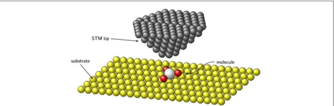
idea by going beyond the linear coupling regime and, more importantly, by considering a non-harmonic, periodic potential energy surfaces associated with a collective rotational degree of freedom rather than with the linear displacement of the standard AHM. Our basic assumption is that the movement of the tip of a Scanning Tunneling Microscope(STM) can act as an effective time-dependent electrical gate for a molecule deposited on the substrate, being able to generate a current-induce rotation. The setup we are envisioning is displayed in figure1: a single molecule adsorbed on a metallic substrate is electrically addressed by the STM tip. This gate is able to change the average occupation of the relevant electronic state coupled to the collective rotational variable (s) and it may thus trigger a (possibly) unidirectional rotation of the molecule. Specifically, we can design two PESs with a given separation of minima and choose an appropriate switching of the gate to make the molecule rotate one-way. To address this problem, we use a quantum–classical approach to the problem, by considering the rotational degrees of freedom as classical variables, whose dynamics is governed by a generalized Langevin equation, while, on the other hand, the electronic system is treated within the nonequilibrium Green function (NEGF) technique exploiting methods developed in the context of current-induced forces [39–45].
The outline of the article is as follows: in section2, the rotational analogy of the AHM Hamiltonian is formulated and the corresponding equation of motion and the reduced density matrix are discussed. In section3, a simple example of a planar molecule with N-fold symmetry is considered. By performing an adiabatic expansion in the reduced density matrix, we derive an equation of motion in the adiabatic limit, which allows simplifying the problem and leading to the concept of mean torque, damping, and external-driving torque. Consequently, it enables one to better estimate the conditions for uni-directional rotation. Finally, in section4we summarize the article and give a brief outlook.
2. Methodology
2.1. General Hamilton operator
Wefirst consider the general Hamilton operator of a molecule of interest, which we can write as: = +
Hmol He Hnuc, where Heand Hnucdescribe the electronic and nuclear degrees of freedom, respectively:
å
= (R ¼ R ) † ( ) He , , d d , 1 n n 1 Na n nå
= P + (R ¼ R ) ( ) H M V 2 , , . 2 i i i N nuc 2 nuc 1 aThe electronic part of the Hamiltonian is written, within a single particle picture, using molecular orbitals and is thus diagonal in this basis.{ }n are the corresponding molecular orbital energies and the operatordn†(dn) creates
(annihilates) an electron in the nth molecular orbital (including spin degrees of freedom). These orbitals in general depend on the individual coordinates of the constitutive Na-atoms{R1,¼,RNa}, meaning that
intramolecular distortions can modify the orbital energies. The nuclear part is treated classically in the spirit of the Born-Oppenheimer approximation by invoking the large mass difference between electrons and nuclei[46].
The variablesPiand Midenote the momentum and mass of the ith nucleus, respectively. In order to address the
rotational dynamics of a molecule deposited on a substrate, we need to compute its potential energy surface in terms of the full set of nuclear coordinates{R1,¼,RNa}and include the influence of the surface; this requires, however, an atomistic approach to the problem, which goes beyond the scope of the current study. To further proceed, we assume that the substrate is acting only as a conformational constraint, so that the dynamics of the molecule on the substrate can be described in terms of only three collective variables: the center of mass coordinates(implying that the internal relative motion is neglected) and two collective angular variables. Thus,
we write the Hamiltonian as:
å
q y q y = + + + q y ( ) † ( ) ( ) ( ) R P L R H d d M I V , , 2 2n , , , 3 n n CM n n CM CM mol 2 mol 2 , nucwhere RCMand Mmolare the center of mass coordinate of the molecule and the total molecular mass,
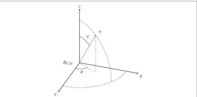
respectively,θ is the azimuthal angle in a plane parallel to the substrate, and ψ is a polar angle or tilt angle with respect to the normal to the substrate(see figure2). Note that these angles can always be clearly defined with
respect to the specific orientation of the molecule in the state with lowest energy. The vectorsLis angular momentum and In(θ, ψ)is the moment of inertia with respect to the principle axisn(q y, ). Clearly, a
more systematic approach would imply an explicit coarse-graining of the full set of molecular coordinates
{Ri} (Nadegrees of freedom) down to a set of few collective variables, going beyondRCM, ,q y[35]. Here,
however, we assume that this has been already carried out and based our choice of the collective coordinates on physical intuition. To further simplify our model, we consider situations where the molecule can not be tilted with respect to the normal to the substrate, thus removing the angular variableψ from our description. If the center of mass is alsofixed by the interaction with the substrate, we are then left with a single angular degree of freedomθ. We can separate the electronic Hamiltonian into a contribution arising from occupied states –up to the highest-occupied molecular orbital(HOMO)–and a contribution from the unoccupied states –beginning with the lowest-unoccupied molecular orbital(LUMO):
å
å
= † + † ( ) He d d d d . 4 m m m m n n n n HOMO LUMOIn general, only orbitals below the LUMO arefilled up. Therefore, the electronic operators are acting on a subspace of the Fock space in which all the occupation numbers below HOMO are equal to 1. As a result, thefirst term in the previous equation becomes a scalar function of the collective variables{RCM, ,q y}, namely
q y
åm m=U0(RCM, , ), which defines the ground state potential energy surface of the molecule. If now additional electrons are added to the molecule, the Hamiltonian in this subspace becomes:
å
= + ( - ) † ( ) He U U U d d , 5 n n n n 0 LUMO 0where Un=òn+U0represents now the potential energy surface with an occupied nth-orbital.
Once this minimal molecular Hamiltonian has been introduced, we can easily extend it to include the coupling to electronic degrees of freedom describing the electronic systems of the substrate and the STM tip:
å
å
å å
= + D + + a a a a a a a ( ) ( ) ( ) † † † Hint c c t d d T c d h c. . 6 k k k k n n n n k n LUMO kn k n LUMOThe molecule is contacted by the STM tip(α=T) and deposited on the substrate (α=S) with the energy spectraòkα, where k stand for the corresponding wave vector. The electronic matrix elementTknadescribes the
coupling between the levels in the molecule and the reservoirs. The operatorsc†a
k and ckαare creation and
annihilation operators of an electron in levelòkα, respectively. The third term in equation(6) mimics the local
electrostatic gating effects coming from the action of the STM tip on the molecule such as consecutive probing; the overall effect is included in a time-dependent gatingΔn(t).
Figure 2. The orientation of the molecule specified by an azimuthal angle θ and polar or tilt angle ψ.
3
2.2. Rotational Anderson-Holstein model(RAHM)
Combining equations(3) and (6), we arrive at the following general Hamiltonian:
= ˜ + ˜ + - ( ) HAHM He Hmol Ve m 7 with
å
å
å å
å
= D + + + = + + = -a a a a a a a q y -˜ ( ) ( ) ˜ ˜ ( ˜ ˜ ) † † † ( ) † P L H t d d c c T c d h c H M I U V U U d d . , 2 2 , , n e n n n n k k k k k n LUMO kn k n CM e m n n n n LUMO mol 2 mol 2 , 0 LUMO 0whereU˜0ºU0+VnucandU˜nºUn+Vnuc. Now,H˜erepresents the effective electronic Hamiltonian relevant
for the dynamics andH˜mis the unperturbed molecular Hamiltonian with effective ground state potential energy
surface ˜U0. The interaction termVe m- , which is crucial in our approach, describes the possibility that the
molecular conformational state can change from its ground state PES ˜U0to any other PESU˜nin dependence on
the occupation of electronic states with energiesnLUMO. Note that the interactionU˜n-U˜0is in general a
non-linear function in the angular variablesθ and Ψ. If the angular distortions and the separation of the two PES minima can be considered as small, then a Taylor expansion can be used to obtain a linear coupling between the angles and the electronic degrees of freedom. In this case, we recover the AHM. However, in our case, where the focus is the possibility of inducing global rotations of the molecule, both the full non-linear potential and the non-linear electron-rotation coupling must be taken into account. Therefore, our model can be viewed as a generalized version of the AHM. For the sake of simplicity, we will drop all the tildes from now on.
To extend the model given by equation(7), one can include the first-order corrections due to the fast nuclear
dynamics in the Hamiltonian, which yields off-diagonal coupling terms. In general, one may also introduce an angle dependence of the molecule-lead coupling strength. This dependence will be determined by the details of the setup, e.g. the geometry of molecule and the tip.
2.3. Langevin equation
Using Hamilton’s equations of motion, we can derive a Langevin equation for the rotational dynamics of the classical variableθ as:
s q q q q q x + ¶ ¶ = -¶ ¶ - + ⎡ ⎣⎢ ⎤ ⎦⎥ (U( ) ( ) ) ˆ ( ) I¨ U0 Tr U0 1 , 8
wheresdenotes the reduced electronic density matrix. We have further introduced a matrixUwith elements given by Umn=Unδmn. In this equation of motion, thefirst term on the right hand side will be denoted as
current-induced torque. It is given by the expectation value of an operator valued torque. The second term, xˆ, which is a stochastic operator, quantifies the deviation of the torque from the mean value. If one assumes that the time scales for the rotational dynamics of the molecule and for the electron transfer from the tip to the molecule are well separated, then the electronic system can always reach a stationary state according to the corresponding molecular configuration. This represents the so called non-equilibrium Born-Oppenheimer (NEBO) approx-imation[40], and one can show that the noise term in the adiabatic limit is always delta-correlated in time. In
order to account for the noise, the operator xˆ is often replaced by a classical stochastic torqueξ(t) with an appropriate correlation function[40,42,43,45]. Note that the damping is implicitly hidden in the first term.
One can perform the adiabatic expansion of the density matrix up tofirst-order to get an explicit expression for the damping, which can be shown to fulfill the fluctuation-dissipation theorem in the limiting case of thermal equilibrium. On the other hand, according to the equation(8) the dynamics of the relevant nuclear degrees of
freedom are mainly determined by an ensemble-averaged PES given on the right-hand side if the torque noise is sufficiently weak. The opposite limit is captured by considering a single-trajectory dynamics, where the switching between potential energy surfaces is purely stochastic[35].
2.4. Electronic dynamics
To actually solve equation(8), we first need to know the reduced density matrix, which can be obtained by
solving the following equation of motion in the time domain[47,48]:
¶s s
å
P P ¶ ( )=[ ( ) ( )]-+ a [ a( )+ a( )] ( ) † H i t t t , t i t t . 9Here,H t( )is the matrix withHmn( )t = D[ n( )t +Un( ( ))q t -U0( ( ))]q t dmnandPaare so-called current
ò
Pa( )t = dt¢[G<(t t, ¢)Sa>(t t¢, )-G>(t t, ¢)S<a(t t¢, )]. (10)
t t
0
HereGandSare lesser/greater Green’s functions and self-energies, respectively [49]. The current matrices
are closely related to the current by:
P
=
a( ) { a( )} ( )
J t 2e Re Tr t , 11
with e denoting the elementary charge. However, in the general case the calculation of the current matrices is very challenging. To overcome this, we consider the wide-band limit[50], where the real part of the retarded
self-energySRis vanishing and the imaginary part is a constant independent of the energy. Then, we can solve the
following system of differential equations to get the reduced density matrix without evaluating the complicated convolution integral in equation(10):
¶s s G s
å
Gå
P ¶ = - - + a a+ = a + ¥ ⎛ ⎝ ⎜⎜ ⎞ ⎠ ⎟⎟ ( ) [H( ) ( )] [ ( )] ( ) ( ) i t t t , t i 2, t i t h c 1 4 p 1 p . . , 12 b c P G G P ¶ ¶ a = a+ - - a+ a ⎡ ⎣⎢ ⎤⎦⎥ ( ) H( ) ( ) i t t R t i 2 , 13 p p p pwhere Gadenotes the broadening matrix with G= åa aG = -2 ImSR, andPap( )t are auxiliary current
matrices, which are related to the current matrix through the relation:
å
s Pa = - Ga+ Pa = ¥ ( )t 1[ ( )]t ( )t ( ) 4 1 2 p 1 p . 14The coefficients Rpand poles c+apare determined by the Matsubara expansion[51] with coefficients Rp=1
and poles capmap(2p-1) /bwhereμαis the chemical potential in reservoirα and 1/β=kBT
represents the thermal energy. For a better convergence, we choose Karrasch’s approach [52] to obtain the
coefficients Rpand poles zp. To get additional insight into the problem, we perform now an adiabatic expansion
of the reduced density matrix and the current matrices[53]:
s=s( )0 +s( )1 +...., (15)
Pap=Pa( )0p+Pa( )1p+... (16) The superscript(n) denotes the n-th order correction with respect to the time derivative. The zeroth-order term is the instantaneous solution of the time-dependent Hamiltonian and thefirst-order term will be related below to the damping and the influence of external driving. We therefore limit or discussion to these two contributions in the expansion and provide analytic expressions for them in the appendixA.
A similar expansion can be carried out for the current Jα(t), giving:
å
å
s s » + = - G + P = - G + P a a a a a a a = ¥ = ¥ ⎛ ⎝ ⎜ ⎜ ⎡ ⎣ ⎢ ⎢ ⎤ ⎦ ⎥ ⎥ ⎞ ⎠ ⎟ ⎟ ⎛ ⎝ ⎜ ⎜ ⎡ ⎣ ⎢ ⎢ ⎤ ⎦ ⎥ ⎥ ⎞ ⎠ ⎟ ⎟ ( ) ( ) ( ) ( ) [ ( )] ( ) ( ) ( ) ( ) ( ) ( ) ( ) ( ) ( ) ( ) ( ) ( ) ( ) J t J t J t J t e t t J t e t t , 2 1 4 1 2 Re , 2 1 2 Re . 17 p p p p 0 1 0 0 1 0 1 1 1 1 whereJa( )0 and a( )J1 are zeroth andfirst-order correction for the current flow out of the reservoir α.
3. A single electronic level coupled to the rotational motion
We apply the formalism presented above to the simple case of a planar molecule with N-fold symmetry placed on top of a metallic substrate and we consider only one relevant electronic level(LUMO) as relevant for the rotational dynamics. In addition, we focus on the current-induced torque only[54], so that the stochastic term is
not considered(Ehrenfest approximation). Since the ground state PES should display the molecular symmetry, we make the Ansatz:
q =t q
( ) ( ) ( )
U0 0sin N , 18
whereτ0gives the amplitude of the angle-dependent potential. We also need to define the PES U1(θ)
corresponding to the excited state with non-zero electron occupancy. The simplest way to describe it is by introducing a phase shift between the two PES[35]:
5
q =t q+f
( ) ( ) ( )
U1 0sin N . 19
Once we specify the molecular potential, we can write down the adiabatic corrections to the reduced density matrix by using the adiabatic expansion; details of the calculations can be found in appendixB. Inserting the obtained reduced density matrix into equation(8), we arrive at an equation of motion for the rotational degree
of freedom of the molecule:
q
q t q t q q t q
+ ¶
¶ = ( )+ ( ˙)+ ( ) ( )
I¨ U0 m d , e ,t . 20
The three terms on the right-hand side are the current-induced mean torque, current-induced damping, and the external-driving torque, respectively, which are given by the expressions:
t q( )= -tN(cos(Nq+f)-cos(Nq s)) ( )( )q , (21) m 0 0 t q q t q f q s q q g q q = - + º -( ˙) ( ( ) ( )) ( ˙) ( ) ˙ ( ) ( ) N N N , cos cos , , 22 d 0 d1 t qe( ,t)= -t0N(cos(Nq+f)-cos(Nq s)) e( )1(q,t). (23) σ(0)is a zeroth-order(adiabatic) contribution to the density matrix, whiles( )
d1 ands
( )
e1 arefirst-order corrections
related to the damping and external driving, respectively(further details are provided in appendixB). Once we
have the equation of motion, we are ready to solve the equation(20); the solutions will be divided into two cases,
depending whether the orbital shift is time-dependent or not.
3.1. Time-independent case
In this case, we consider a planar molecule with a three-fold symmetry(N=3), which experiences a constant orbital shiftΔ(t)=const. One can immediately find that the external-driving torque vanishes according to equation(B.2). To solve the equation of motion, we use the following parameters which are representative of
typical experimental conditions[14–16,35,55]: T=5 K, f=π/2, I=10−42kg·m2,Δμ=μT−μS=
10 meV,τ0=10 meV and Γ=0.1 meV. For the initial condition, we set θ(0)=−π/4 and q˙ ( )0 =0 rad . ns./
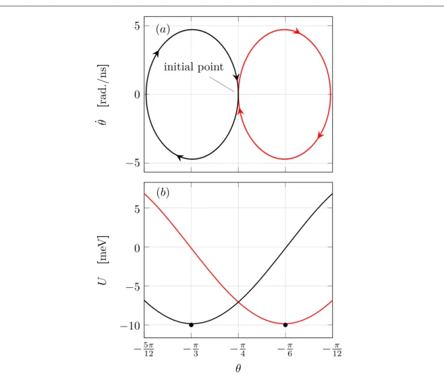
By solving the adiabatic Langevin equation, we can obtain the phase-space trajectory of the solution, which is shown infigure3(a). The red (black) line represents the solution with the orbital shift Δ=1 eV (−1 eV) and the
solution exhibits a typical damped oscillation behavior with correspondingfixed-points atq=q*L andq*R (close to −π/3 and −π/6 respectively).
To explain this oscillatory behavior, we rewrite equation(20) as follows:
q
q g q q
= -¶
¶ - ( ) ˙ ( )
I¨ Ueff 24
with the effective potentialUeff( )q =U0( )q -
ò
qqt qm( )¢ dq¢0
. From equation(24), one can understand that the
molecule is rotating according to the effective potential with an angle-dependent dampingγ(θ), which are shown infigure3(b). In terms of the effective potential, it is easy to explain why the fix-points are atq=q*L andq*R: when the orbital shift is high(Δ=1 eV), the corresponding electron density on the molecule is nearly zero. According to our previous discussion when introducing the RAHM, we know that in this case Ueff(θ)≈U0(θ).
As a result, the molecule starts to change the orientation until it reaches the nearest local minimum on the effective potential surface, which is simply at *qR(fixed-point on the right). On the contrary, if the orbital shift is low(Δ=−1 eV), the average electron occupation approaches unity, which implies Ueff(θ)≈U1(θ), so that the
nearest local minimum is atq*Lin this case. 3.2. Time-dependent case
In the previous section, we have already seen that the location of thefixed-points depends on the orbital shift. This suggests that a time-dependent orbital shift may be considered a way to manipulate the location of the fixed-points, i.e. to control the rotational behavior of the molecule. Here, we assume the following orbital shift (see figure4): D = -+ D -( ) ( ) ( ) ( ) t e e 1 1 , 25 k t t k t t 1 1
whereΔis the initial orbital shift; k is the switching rate of the orbital shift and t1is the switching time.
In the following calculations, we use the parametersf=−11π/12, k=100 GHz, Δ=1 eV, I=10−41kg·m2
,Δμ=μL−μR=10 meV, τ0=10 meV, Γ=0.1 eV and t1=100 ps [14–16,35,55]. For
the initial conditions, we chooseθ(0)=θ*,σ(0)=σ(0)(θ*) andPap( )0 = Pa( )0p(q*), which means that the
molecule starts from one of thefixed-points. One can clearly see in figure4(b) that as Δ(t) decreases the electron
occupation increases. The time-dependency of the total currentflow into the molecule JL+JRis also consistent
hand, the trajectory infigure4(d) shows a similar oscillatory behavior as in the time-independent case. From the
pattern of the phase-space trajectory, it is straightforward to consider a consecutive switching of orbital shift to see whether an open trajectory is possible, which would mean that the molecule is rotating uni-directionally instead of oscillating around a local minimum. To implement consecutive switching, we apply the following time-dependent orbital shift:
Figure 3. Solution of equation of motion with parametersf=π/2, I=10−42kg·m2,μL=−μR=5 meV, τ0=10 meV and
Γ=0.1 eV. The initial conditions are θ(0)=−π/4 andq˙ ( )0 =0. The red(black) line represents the solution with the orbital shift Δ=1 eV (−1 eV). (a) Phase-space trajectory. The black point marks the initial starting point. (b) Effective potential. The black points mark thefixed-points on the rightq*Rand left *qL.
Figure 4. Solution of time-dependent orbital shift with parametersf=−11π/12, I=10−41kg·m2,Δμ=μL−μR=10 meV,
τ0=1 meV and Γ=0.1 eV for different types of switching. Figures (a)–(d) show the time-dependency of orbital shift, electron
density, total currentflow into the molecule and phase-space trajectory for single-switching with switching timing t1=100 ps,
respectively. In the bottom,figures (e)–(h) illustrate the same quantities with two switching timing t1=100 ps and t2=400 ps.
7
D = + - + + D - -⎡ ⎣⎢ ⎤ ⎦⎥ ( ) ( ) ( ) ( ) t e e 2 1 2 1 1 , 26 k t t1 k t t2
with t1=100 ps and t2=400 ps. Due to the second switch, the instantaneous change of the fixed-point can
possibly make the molecule rotate one-way. To achieve this kind of rotation, the switching timing has to be in coherent with the instantaneous angular velocity; otherwise, the molecule is not able to cross the nearby potential maximum and it will hence display an oscillatory behavior. Infigure4(h), since the second switch is
coherent, the trajectory becomes open, which means the rotation is uni-directional. Note that, in our approach, the rotation is driven by manipulating the electrostatic gating effect explicitly instead of using a stochastic driving torque[35].
3.2.1. Response to different phase-shifts
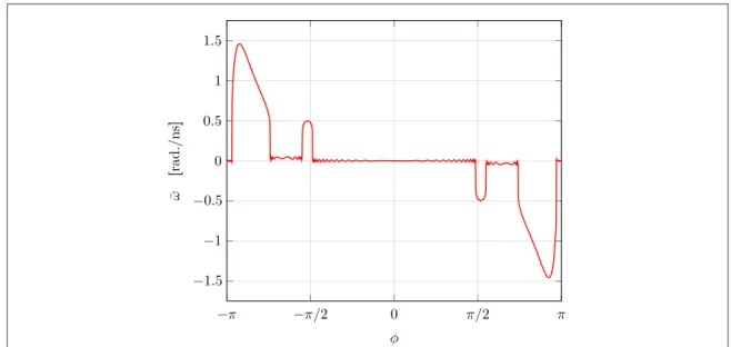
An interesting issue is whether a phase shiftf between the two PES may be found, such that the molecule will rotate with the largest angular velocity. To answer this question, we have used the same parameters as for the time-dependent case while adjusting the phase-shift from−π to π to see the behavior of the average angular velocity6w¯. Infigure5, one can clearly see that there exist certain windows in the values of the phase shift where the angular velocity of the molecule is in resonance with the external switching. We therefore denote this behavior as resonant rotation. The response is fully anti-symmetric with respect tof=0, since the ground state PESU0=t0sin 3qis also anti-symmetric. Infigure5there are peaks close to±π and ±π/2. The direction of the rotation forf close to −π can be explained by considering the effective potential U1. Suppose t<t1, then the
molecule is always staying on a minimum of the PES. When t1<t<t2it is moving to a nearby minimum of
t q p
= ( - )
U1 0sin 3 11 12, which is on the right-hand side of the original location. For t>t2, the potential is
then switched back to U0, but the angular velocity is large enough such that the molecule can further rotate in the
same direction, which is similar to the scenario infigure4(h). For the peaks near f≈−π/2, the mechanism is
similar. The only difference is that the second switching takes place before the molecule crosses thefirst local maximum in the U0surface forf≈−π, whereas the second switching happens after the molecule passes the
first local maximum in the U0surface forf≈−π/2.
4. Conclusion
We have proposed a rotational version of the Anderson-Holstein model to describe the molecular rotational dynamics in a generic setup consisting of a single molecule adsorbed on a metallic substrate and electrically addressed by an STM tip. By applying an adiabatic expansion to the time-evolution of the reduced density matrix, the damping and external driving can be related to thefirst-order corrections of the reduced density matrix. To demonstrate our approach, a planar molecule with N-fold spatial symmetry was considered, where a single rotational variable couples non-linearly to an electronic level, the occupation of the latter being controlled
Figure 5. Phase response of molecular average angular velocity w¯ with parameters I=10−41kg·m2,Δμ=μ
L−μR=10 meV,
τ0=1 meV and Γ=0.1 eV with two switching timing t1=100 ps and t2=400 ps.
6
by a local, in general time-dependent gate mimicking the influence of current pulses coming from the STM tip. We have shown that unidirectional rotation can be achieved by specific tuning of the time-dependent gate as well as of the relative phase difference of the potential energy surfaces. Our framework can be systematically extended to include multi-level electronic systems as well as more than one collective variable. It thus opens the possibility to make contact with atomistic simulations able to provide quantitative information e.g. on the shape of the potential energy surfaces involved in the rotational process[11] and on the strength of the coupling between
mechanical and electronic degrees of freedom. On this basis, a further going step would be the study of the mechanisms leading to the transmission of angular momentum in coupled molecular rotor arrays, which represents a major issue in designing molecule-based mechanical devices.
Acknowledgments
We would like to thank H-L Yang, T Lehmann, P Goldberg, M Bobeth, and R Biele for very useful discussions and suggestions. This work has been supported by the European Union Horizon 2020 FET open project Mechanics with Molecules(MEMO, grant nr. 766864).
Appendix A. Adiabatic expansion
In order to further simply the problem, we consider the adiabatic approximation, the reduced density matrix can be expanded by the following:
s=s( )0 +s( )1 +.... (A.1) Similarly, this also holds for the auxiliary current matrices:
Pap =Pa( )0p +Pa( )1p +.... (A.2)
A.1. Zeroth-order correction
For simplicity, we setÿ=1 in the following. The zeroth-order correction s( )0 and P
a
( )
p
0 can be obtained by
solving the following equation:
s P ¶ ¶ = ¶ ¶ = a ( ) ( ) ( ) i t p i t 0. A.3 0 0
Then we can immediately obtain
b c Pa = - - G- a+ Ga -⎡ ⎣⎢ ( ) ⎤⎦⎥ ( ) ( ) H R t i 2 . A.4 p p p 0 1
Then the reduced density matrix can be obtained by solving the so-called Sylvester equation:
å
s s G G G G - - + = - + a a a a a ( ) ( ) ( )( ) ( †) ( ) H i 2 0 0 H i 2 i F F A.5 whereå
b G c = - - -a a+ -⎡ ⎣⎢ ⎤⎦⎥ ( ) F 1 R H i 4 p 2 . A.6 p p 1A.2. First-order correction
For thefirst-order correction, by plugging the zeroth-order corrections s( )0 and P
a
( )
p
0 into equations(13), (12)
and neglecting the derivative of thefirst-order terms Then we have the following equation:
c P = - G- ¶P ¶ a a+ a -⎡ ⎣⎢ ⎤ ⎦⎥ ( ) ( ) ( ) ( ) H t i i t 2 , A.7 p p p 1 1 0
å
s s s G G P - - + = ¶ ¶ - a a (H i ) ( ) ( )(H i ) i ( ) ( ) ( ) t i 2 2 2 Re . A.8 p p 1 1 0 1As in zeroth-order case, the equations above enable one to get thefirst-order corrections. 9
Appendix B. Density matrix for the single-level planar molecule
We show the analytic solutions of equations(A.5) and (A.8) for the planar molecule. The zeroth and first-order
terms are given by:
å
s p b p t q f q m b p b p t q f q m b p = - Y - + - + D - + G - Y + + - + D - + G a a a = ⎜ ⎟ ⎜ ⎟ ⎡ ⎣⎢ ⎛ ⎝ ⎞⎠ ⎛ ⎝ ⎞⎠ ⎤ ⎦⎥ ( ( ( ) ( ) ( )) ) ( ( ( ) ( ) ( )) ) ( ) ( ) i i N N t i N N t 1 2 4 1 2 2 sin sin 4 1 2 2 sin sin 4 , B.1 L R 0 , 0 0å
å
s b t q f q q p b p t q f q m b p b p t q f q m b p t q f q q b t q f q c q q q s q q s q = + - + D G ´ Y¢ - + - + D - + G + Y¢ + + - + D - + G - + - + D ´ + - + D - G -= + D º + a a a a a+ ⎜ ⎟ ⎜ ⎟ ⎡ ⎣⎢ ⎛ ⎝ ⎞⎠ ⎛ ⎝ ⎞ ⎠ ⎤ ⎦⎥ ⎛ ⎝ ⎜⎜ ⎞⎠⎟⎟ [ ( ( ) ( )) ˙ ˙ ( )] ( ( ( ) ( ) ( )) ) ( ( ( ) ( ) ( )) ) ( ( ) ( )) ˙ ˙ ( ) [ ( ( ) ( ) ( ) ] ( ) ˙ ( ) ˙ ( ) ( ˙) ( ) ( ) ( ) ( ) ( ) N N N t i N N t i N N t N N N t R N N t i f f t t cos cos 8 1 2 2 sin sin 4 1 2 2 sin sin 4 cos cos Im sin sin 2 , , . B.2 p p p d e 1 0 2 0 0 0 , 0 3 1 2 1 1Note that the digamma function is defined as Y( )z º d ln( ( ))G z
dz , whereΓ(z) is the Gamma function. For
thefirst-order correction, we have defined two terms in the right-hand side of equation (B.2). The first term
s( )d1(q q,˙ )is called the damping term, which is proportional to the angular velocity q˙. On the other hand, the second terms( )e1(q,t), is the external-driving term proportioned to the time derivative of orbital shift D˙ ( )t .
ORCID iDs
R Gutierrez https://orcid.org/0000-0001-8121-8041
References
[1] Gimzewski J K and Joachim C 1999 Science283 1683–8
[2] Feringa B L 2017 Angew. Chemie Int. Ed.56 11060–78
[3] Saywell A, Bakker A, Mielke J, Kumagai T, Wolf M, García-López V, Chiang P T, Tour J M and Grill L 2016 ACS Nano10 10945–52
[4] van Leeuwen T, Lubbe A S, Štacko P, Wezenberg S J and Feringa B L 2017 Nat. Rev. Chem.1 0096
[5] Kelly T R, De Silva H and Silva R A 1999 Nature401 150–2
[6] Tierney H L, Murphy C J, Jewell A D, Baber A E, Iski E V, Khodaverdian H Y, McGuire A F, Klebanov N and Sykes E C H 2011 Nat. Nanotechnol.6 625–9
[7] Michl J and Sykes E C H 2009 ACS Nano3 1042–8
[8] Santamato E, Daino B, Romagnoli M, Settembre M and Shen Y R 1986 Phys. Rev. Lett.57 2423–6
[9] Roegel D 2015 IEEE Ann. Hist. Comput.37 90–6
[10] Nickel A, Ohmann R, Meyer J, Grisolia M, Joachim C, Moresco F and Cuniberti G 2013 ACS Nano7 191–7
[11] Mishra P et al 2015 Nano Lett.15 4793–8
[12] Stipe B C 1998 Science279 1907–9
[13] Pawin G, Stieg A Z, Skibo C, Grisolia M, Schilittler R R, Langlais V, Tateyama Y, Joachim C and Gimzewski J K 2013 Langmuir29 7309–17
[14] Eisenhut F, Meyer J, Krüger J, Ohmann R, Cuniberti G and Moresco F 2018 Surf. Sci.678 177–182
[15] Moresco F 2004 Phys. Rep.399 175–225
[16] Moresco F 2015 Driving molecular machines using the tip of a scanning tunneling microscope Joachim C., Rapenne G. Single Mol. Mach. Mot. Adv. Atom Single Mol. Mach.(Cham: Springer) pp 165–86
[17] Kudernac T, Ruangsupapichat N, Parschau M, MacIá B, Katsonis N, Harutyunyan S R, Ernst K H and Feringa B L 2011 Nature479 208–11
[18] Natterer F D, Patthey F and Brune H 2013 Phys. Rev. Lett.111 175303
[19] Jung T A, Schlittler R R and Gimzewski J K 1997 Nature386 696–8
[20] Manzano C, Soe W H, Wong H S, Ample F, Gourdon A, Chandrasekhar N and Joachim C 2009 Nat. Mater.8 576–9
[21] Perera U G, Ample F, Kersell H, Zhang Y, Vives G, Echeverria J, Grisolia M, Rapenne G, Joachim C and Hla S W 2013 Nat. Nanotechnol.
8 46–51
[22] Li C, Wang Z, Lu Y, Liu X and Wang L 2017 Nat. Nanotechnol.12 1071–6
[24] Fennimore A M, Yuzvinsky T D, Han W Q, Fuhrer M S, Cumings J and Zettl A 2003 Nature424 408–10
[25] Barreiro A, Rurali R, Hernandez E R, Moser J, Pichler T, Forro L and Bachtold A 2008 Science320 775–8
[26] Lotze C, Corso M, Franke K J, von Oppen F and Pascual J I 2012 Science338 779–82
[27] Kim K, Xu X, Guo J and Fan D L 2014 Nat. Commun.5 3632
[28] Bustos-Marún R, Refael G and Von Oppen F 2013 Phys. Rev. Lett.111 1–5
[29] Fernández-Alcázar L J, Pastawski H M and Bustos-Marún R A 2017 Phys. Rev. B95 1-12
[30] Croy A and Eisfeld A 2012 EPL (Europhysics Lett.)98 68004
[31] Bruch A, Kusminskiy S V, Refael G and Von Oppen F 2018 Phys. Rev. B97 1–12
[32] Fernández-Alcázar L J, Bustos-Marún R A and Pastawski H M 2015 Phys. Rev. B—Condens. Matter Mater. Phys.92 1–7
[33] Calvo H L, Ribetto F D and Bustos-Marún R A 2017 Phys. Rev. B96 165309
[34] Arrachea L and von Oppen F 2015 Phys. E Low-dimensional Syst. Nanostructures74 596–602
[35] Echeverria J, Monturet S and Joachim C 2014 Nanoscale6 2793
[36] Anderson P W 1961 Phys. Rev.124 41–53
[37] Holstein T 1959 Ann. Phys. (N.Y)8 325–42
[38] Hewson A C and Meyer D 2002 J. Phys. Condens. Matter14 427
[39] Di Ventra M, Chen Y C and Todorov T N 2004 Phys. Rev. Lett.92 176803
[40] Bode N, Kusminskiy S V, Egger R and von Oppen F 2011 Phys. Rev. Lett.107 036804
[41] Bode N, Kusminskiy S V, Egger R and von Oppen F 2012 Beilstein J. Nanotechnol.3 144–62
[42] Dundas D, McEniry E J and Todorov T N 2009 Nat. Nanotechnol.4 99–102
[43] Lü J T, Brandbyge M and Hedegård P 2010 Nano Lett.10 1657–63
[44] Todorov T N, Dundas D, Paxton A T and Horsfield A P 2011 Beilstein J. Nanotechnol.2 727–33
[45] Todorov T N, Dundas D, Lü J T, Brandbyge M and Hedegård P 2014 Eur. J. Phys.35 065004–23
[46] Born M and Oppenheimer R 1927 Ann. Phys.389 457–84
[47] Croy A and Saalmann U 2009 Phys. Rev. B80 245311
[48] Zheng X, Wang F, Yam C Y, Mo Y and Chen G 2007 Phys. Rev. B—Condens. Matter Mater. Phys.75 1–16
[49] Haug H and Jauho A P 2008 Quantum kinetics in transport and optics of semiconductors Solid-State Sciences vol 123 (Berlin, Heidelberg: Springer)
[50] Verzijl C J O, Seldenthuis J S and Thijssen J M 2013 J. Chem. Phys.138 094102–23
[51] Mahan G D 1990 Many-Particle Physics (Boston, MA: Springer US) [52] Karrasch C, Meden V and Schönhammer K 2010 Phys. Rev. B82 125114
[53] Entin-Wohlman O, Aharony A and Levinson Y 2002 Phys. Rev. B65 195411
[54] Hussein R, Metelmann A, Zedler P and Brandes T 2010 Phys. Rev. B82 165406
[55] Garrigues A R, Yuan L, Wang L, Mucciolo E R, Thompon D, Barco E and Nijhuis C A 2016 Sci. Reports1–15
11