HAL Id: hal-02154992
https://hal.archives-ouvertes.fr/hal-02154992
Submitted on 18 Dec 2019HAL is a multi-disciplinary open access
archive for the deposit and dissemination of sci-entific research documents, whether they are pub-lished or not. The documents may come from teaching and research institutions in France or
L’archive ouverte pluridisciplinaire HAL, est destinée au dépôt et à la diffusion de documents scientifiques de niveau recherche, publiés ou non, émanant des établissements d’enseignement et de recherche français ou étrangers, des laboratoires
A First Step Toward Computing All Hybridization
Networks For Two Rooted Binary Phylogenetic Trees
Celine Scornavacca, Simone Linz, Benjamin Albrecht
To cite this version:
Celine Scornavacca, Simone Linz, Benjamin Albrecht. A First Step Toward Computing All Hybridiza-tion Networks For Two Rooted Binary Phylogenetic Trees. Journal of ComputaHybridiza-tional Biology, Mary Ann Liebert, 2012, 19 (11), pp.1227-1242. �10.1089/cmb.2012.0192�. �hal-02154992�
A first step towards computing all
hybridization networks for two rooted binary
phylogenetic trees
Celine Scornavacca
∗,
†Simone Linz
∗,‡Benjamin Albrecht
§February 10, 2015
Abstract
Recently, considerable effort has been put into developing fast algo-rithms to reconstruct a rooted phylogenetic network that explains two rooted phylogenetic trees and has a minimum number of hybridiza-tion vertices. With the standard approach to tackle this problem be-ing combinatorial, the reconstructed network is rarely unique. From
∗Equally contributing authors.
†C. Scornavacca is at the ISEM, UMR 5554, Universit´e Montpellier II. Montpellier,
France. [email protected]
‡Simone Linz is at the Biomathematics Research Centre, University of Canterbury.
Christchurch, New Zealand [email protected]
§Benjamin Albrecht is at the Institut of Informatics, Ludwig Maximilians University.
a biological point of view, it is therefore of importance to not only compute one network, but all possible networks. In this paper, we make a first step towards approaching this goal by presenting the first algorithm—called allMAAFs—that calculates all maximum-acyclic-agreement forests for two rooted binary phylogenetic trees on the same set of taxa.
Keywords: Directed acyclic graphsHybridizationMaximum-acyclic-agreement forests-Bounded searchPhylogenetics
1
Introduction
Over the last decade, significant progress in phylogenetic studies has been achieved by combining the expertise acquired in the fields of biology, com-puter science, and mathematics. As for the latter, combinatorics is becom-ing increasbecom-ingly important in approachbecom-ing many problems in the context of reticulate evolution (e.g., see [? ? ] for two excellent reviews) which is an umbrella term for processes such as horizontal gene transfer, hybridization, and recombination. To analyze reticulation in evolution, the graph-theoretic concept of an agreement forest for two rooted phylogenetic trees has at-tracted much attention (e.g. [? ? ? ? ? ]). However, most approaches that make use of this concept aim at quantifying the amount of reticulation that is needed to simultaneously explain a set of rooted phylogenetic trees. Thus, one is primarily interested in the number of horizontal gene transfer, hybridization, or recombination events that occurred during the evolution of a set of present-day species. Consequently, these approaches do not explicitly
construct a rooted phylogenetic network that explains a set of phylogenetic trees. Nevertheless, this is desirable from a biological point of view because such a network intuitively indicates how species may have evolved by means of speciation and reticulation. While each vertex of a phylogenetic tree has exactly one direct ancestor, a vertex of a phylogenetic networks may have more than one such ancestor; thereby indicating that the genome of the un-derlying species is a combination of the genomes of distinct parental species. Generically, we refer to such a vertex as a reticulation vertex or, more specific in the context of hybridization, as a hybridization vertex. Since reticulation events are assumed to be significantly less frequent than speciation events, current research aims at constructing a rooted phylogenetic network that ex-plains a set of rooted phylogenetic trees and whose number of reticulation vertices is minimized.
For the purpose of the introduction, think of a so-called maximum-acyclic-agreement forest F for two rooted binary phylogenetic trees S and T as a small collection of vertex-disjoint rooted subtrees that are common to S and T (for details, see Section 2). It is well-known that the size of F minus 1 equates to the minimum number of hybridization events that are needed to explain S and T [? ]. Furthermore, there exists an algorithm—called Hy-bridPhylogeny [? ]—that glues together the elements of F by introducing new edges such that the resulting graph is a rooted phylogenetic network that explains S and T and has ∣F ∣ − 1 hybridization vertices. However, until now, HybridPhylogeny, has not found its way into many practical ap-plications that are concerned with reconstructing the evolutionary history for a set of species whose past is likely to include hybridization. This might
be due to the fact that the reconstructed phylogenetic network is rarely unique because the gluing step can often be done in a number of different ways. Furthermore, given two rooted binary phylogenetic trees S and T , a maximum-acyclic-agreement forest for S and T is rarely unique. Given these hurdles, an appealing open problem is the reconstruction of all rooted phylogenetic networks that explain a pair of rooted phylogenetic trees and whose number of hybridization vertices is minimized. Once having calculated the entire solution space of these networks, one can then for example apply statistical methods or additional biological knowledge to decide which of the phylogenetic network in this space is most likely to be the correct one.
In this paper, we focus on a first step to reach this goal. In particular, we give the first non-naive algorithm—called allMAAFs—that is based on a bounded-search type idea and calculates all maximum-acyclic-agreement forests for two rooted binary phylogenetic trees S and T on the same set of taxa. With the underlying optimization problem being NP-hard [? ] and fixed-parameter tractable [? ], the running time of allMAAFs is expo-nential. More precisely, we will see in Section 5 that the running time of allMAAFs, which is O(3n), can be improved to O(314k+p(n)) by applying the kernelization rules of [? ], where n is the number of leaves in S and T , p(n) is some polynomial function that depends on n, and k is the minimum number of hybridization events needed to explain S and T .
While the description of allMAAFs is slightly complex in comparison to other straight-forward approaches (for more details, see Section 5), it has been shown in a recent paper by ? ], which contains the description of a practical implementation of allMAAFs but without providing any
theoretical background or mathematical justifications, that this algorithm is remarkably quick in practice. Therefore, this paper also aims at establishing the correctness of the algorithm presented in [? ].
The paper is organized as follows. The next section contains preliminaries and some well-known results from the phylogenetics literature. Section 3 describes the algorithm allMAAFs that calculates all maximum-acyclic-agreement forests for two rooted binary phylogenetic trees. Its pseudocode is also given in this section. Subsequently, in Section 4, we establish the correctness of allMAAFs and give its running time in Section 5. We finish the paper with some concluding remarks in Section 6.
2
Preliminaries
In this section, we give some preliminary definitions that are used through-out this paper. Notation and terminology on phylogenetic trees and networks follow [? ] and [? ], respectively.
Phylogenetic trees. A rooted phylogenetic X -tree T is a connected graph with no (undirected) cycle, no vertices of degree 2, except for the root which has degree at least 2, and such that each element of X labels a leaf of T . The set X represents a collection of present-day taxa and internal vertices represent putative speciation events. A rooted phylogenetic X -tree T is said to be binary if its root vertex has degree two while all other interior vertices have degree three. We denote the edge set of T by E(T ). The taxa set X of T is called the label set of T and is frequently denoted by L(T ).
Furthermore, let v be a vertex of T . We denote by L(v) the label set of the rooted phylogenetic tree with root v that has been obtained from T by deleting the edge ending in v. Lastly, let F be a set of rooted phylogenetic trees. Similarly to L(T ), we use L(F ) to denote the union of leaf labels over all elements in F .
We next introduce several types of subtrees that will play an important role in this paper. Let T be a rooted phylogenetic X -tree, and let X′⊂ X be a subset of X . We use T (X′)to denote the minimal connected subgraph of T that contains all leaves that are labeled by elements of X′. Furthermore, the restriction of T to X′, denoted by T ∣X′, is defined as the rooted phylogenetic
tree that has been obtained from T (X′)by suppressing all non-root degree-2 vertices. Lastly, we say that a subtree of T is pendant if it can be detached from T by deleting a single edge.
Now, let T be a rooted binary phylogenetic X -tree, and let X′ be a sub-set of X . Then, the lowest common ancestor of X′ in T is the vertex v in T with X′⊆ L(v) such that there exists no vertex v′ in T with X′ ⊆ L(v′) and L(v′) ⊂ L(v). We denote v by lcaT(X′).
Hybridization networks. Let X be a finite set of taxa. A rooted phylogenetic network on X is a rooted acyclic digraph with no vertex of both indegree and outdegree one and whose leaves are bijectively labeled by elements of X . Since this paper is concerned with hybridization as a representative of reticulation, we will often refer to a phylogenetic network as a hybridization network. Each internal vertex of a hybridization network
with indegree 1 represents a putative speciation event while each vertex with indegree of at least 2 represents a hybridization event and, therefore, a species whose genome is a chimaera of its parents’ genomes. Generically, we call a vertex of the latter type a hybridization vertex and each edge that enters a hybridization vertex a hybridization edge.
To quantify the number of hybridization events, the hybridization number of N , denoted by h(N ), is defined as
h(N ) = ∑
v∈V (N)∶δ−(v)>0
(δ−(v) − 1) = ∣E(N )∣ − ∣V (N )∣ + 1,
where V (N ) and E(N ) denote respectively the vertex and edge set of N and δ−(v) the indegree of v. Note that, if N is a rooted phylogenetic tree, then h(N ) = 0, and if δ−(v) is at most 2 for each vertex v ∈ V (N ), then h(N ) is equal to the total number of hybridization vertices of N .
Now, let N be a phylogenetic network on X , and let T be a rooted binary phylogenetic X′-tree with X′ ⊆ X. We say that T is displayed by N if T can be obtained from N by deleting a subset of its edges and any resulting degree-0 vertices, and then contracting edges. Intuitively, if N displays T , then all of the ancestral relationships visualized by T are visualized by N . In the remainder of this paper, we will consider the case where T is composed of two rooted binary phylogenetic trees.
Extending the definition of the hybridization number to two rooted binary phylogenetic X -trees S and T , we set
h(S, T ) = min{h(N ) ∶ N is a hybridization network that displays S and T }. Calculating h(S, T ) for two rooted binary phylogenetic X -trees has been
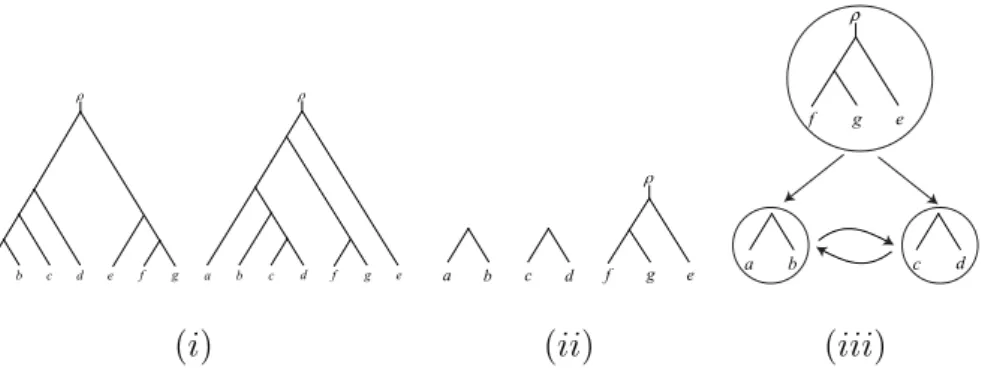
e d c b a f g a b c d f g e a b c d f g e a b c d e g f ρ
(i) (ii) (iii)
Figure 1: (i) Two phylogenetic trees S and T on X = {a, b, c, d, e, f, g}. (ii) An agreement forest F for S and T . (iii) The graph AG(S, T, F ). Since this graph contains a directed cycle, F is not an acyclic-agreement forest for S and T .
shown to be NP-hard [? ].
Forests. Let T be a rooted binary phylogenetic X -tree whose edge set is E(T ). For the purpose of the upcoming definitions and, indeed, much of the paper, we regard the root of T as a vertex labeled ρ at the end of a pendant edge adjoined to the original root of T . For an example of two such trees, see Figure 1(i). Furthermore, we view ρ as an element of the label set of T ; thus L(T ) = X ∪ {ρ}. Any collection of rooted binary phylogenetic trees whose union of label sets is L(T ) is a forest on L(T ). Furthermore, we say that a set F = {F0, F1, . . . , Fk} of rooted binary phylogenetic trees, with ∣F ∣ referred to as the size of F , is a forest for T if F can be obtained from T by deleting a k-sized subset E of E(T ) and, subsequently, suppressing vertices with both indegree and outdegree 1. To ease reading, we write F = T − E if F can be obtained in this way. Obviously, in the same way, we obtain a new forest F′= {F0′, F1′, . . . , Fk′′}for T from F by deleting a k
⋃Fi∈FE(Fi) and, again, suppressing vertices with both indegree and
outde-gree 1. Similarly to the above, we write F′ = F −E′ if F′ can be obtained in this way. Now, let F be a forest for a rooted binary phylogenetic X -tree. We use F to denote the forest obtained from F by deleting all of its isolated vertices and, additionally, the element that contains the vertex labeled ρ if it contains at most one edge. Lastly, for two leaf vertices a and c with labels L(a) and L(c) respectively, we write a ∼F c if there exists an element in F
that contains a leaf labeled with L(a) and a distinct leaf labeled with L(c), otherwise, we write a ≁F c.
Let S and T be two rooted binary phylogenetic X -trees. A set F = {Fρ, F1, F2, . . . , Fk} of rooted phylogenetic trees is an agreement forest for S and T if F is a forest for S and T , and ρ ∈ L(Fρ). Note that the beforehand
given definition is equivalent to the definition of an agreement forest that is usually used in the literature and that we give next. An agreement forest F = {Fρ, F1, F2, . . . , Fk} for S and T is a collection of trees such that the following properties are satisfied:
(i) The label sets L(Fρ), L(F1), L(F2), . . . , L(Fk)partition X ∪ {ρ} and, in particular, ρ ∈ L(Fρ).
(ii) For each i ∈ {ρ, 1, 2, . . . , k}, we have Fi ≅S∣L(Fi)≅T ∣L(Fi).
(iii) The phylogenetic trees in {S(L(Fi)) ∣i ∈ {ρ, 1, 2, . . . , k}} and {T (L(Fi)) ∣ i = {ρ, 1, 2, . . . , k}} are vertex-disjoint subtrees of S and T , respectively. Both definitions of an agreement forests for two rooted binary phylogenetic trees are used interchangeably throughout this paper.
An agreement forest with the minimum cardinality among all agreement forests for S and T is called a maximum-agreement forest for S and T . An example of an agreement forest for the two trees S and T presented in Fig-ure 1(i), is shown in (ii) of the same figFig-ure. It is easy to check that this forest is in fact a maximum-agreement forest for S and T .
A characterization of the hybridization number h(S, T ) for two rooted binary phylogenetic trees S and T in terms of agreement forests requires an additional condition. Roughly, this condition avoids that species can inherit genetic material from their own offsprings. Let F = {Fρ, F1, F2, . . . , Fk} be an agreement forest for two rooted binary phylogenetic X -trees S and T . Furthermore, let AG(S, T, F ) be the directed graph whose vertex set is F and for which (Fi, Fj) is an arc precisely if i ≠ j, and either
(1) the root of S(L(Fi))is an ancestor of the root of S(L(Fj))in S, or (2) the root of T (L(Fi))is an ancestor of the root of T (L(Fj)) in T . We call F an acyclic-agreement forest for S and T if AG(S, T, F ) does not contain any directed cycle. To illustrate, Figure 1(iii) shows the graph AG(S, T, F ) for S, T , and F of the same figure. Note that F is not an acyclic-agreement forest for S and T . Similarly to the definition of a maximum-agreement forest, an acyclic-maximum-agreement forest for S and T whose number of components is minimized over all such forests is called a maximum-agreement forest for S and T . The importance of the concept of acyclic-agreement forests lies in the following theorem that has been established in [? , Theorem 2] and gives an attractive characterization of the hybridiza-tion number for two rooted binary phylogenetic trees.
Theorem 1. Let F = {Fρ, F1, F2, . . . , Fk} be a maximum-acyclic-agreement
forest for two rooted binary phylogenetic X -trees S and T . Then h(S, T ) = k.
In the proof of Theorem 1, the authors implicitly show that, by deleting all hybridization edges of a hybridization network N that displays two rooted binary phylogenetic X -trees S and T and has a minimum number of hy-bridization vertices and, subsequently, suppressing all non-root degree-2 ver-tices, one obtains a maximum-acyclic-agreement forest F for S and T . Note that F is well-defined if N is given. We say that N yields F . On the other hand, given a maximum-acyclic-agreement forest F for two rooted binary phylogenetic X -trees S and T , and using the algorithm HybridPhy-logeny (for details, see [? ]) to construct a hybridization network N from F that displays S and T and yields F , N is rarely unique. Nevertheless, if one aims at reconstructing all hybridization networks that display S and T and whose hybridization number is minimized, one can first calculate all maximum-acyclic-agreement forests for S and T and then construct all pos-sible minimum hybridization networks for each such forest. As mentioned in the introduction, this paper focuses on the first step of this approach, i.e. finding all maximum-acyclic-agreement forests for S and T .
Now, let F be a set of rooted binary phylogenetic trees, and let a and c be two distinct leaves of F . We say that a and c form a cherry in F if they are adjacent to a common vertex, in which case we denote this cherry by {a, c}. Note that a and c refer to leaf vertices and not leaf labels. Let
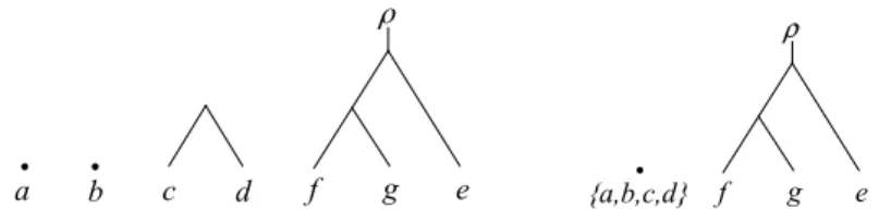
{f,g} e d c b a {f,g} a b c d e
Figure 2: The two phylogenetic trees obtained by calling cherryReduc-tion(S, T , ∅, {f, g}), where S and T are the two phylogenetic trees shown Figure 1(i).
S and T be two rooted binary phylogenetic X -tree, and let F be a forest for T . Furthermore, let {a, c} be a cherry of S∣L(F). We say that {a, c} is a contradicting cherry of S and F if there is no cherry {a′, c′} in F such that one of a′ or c′, say a′, is labeled L(a) while c′ is labeled L(c). Otherwise, we call {a, c} a common cherry of S and F .
Cherry reduction. Let F be a forest for a rooted binary phylogenetic tree, and let {a, c} be a cherry of F . The operation of deleting the two leaf vertices a and c and their respective labels and labeling the resulting new leaf vertex with L(a) ∪ L(c) is called a cherry reduction. The new la-bel L(a) ∪ L(c) is sometimes referred to as a dummy taxon. We denote this reduction by F [{L(a), L(c)} → L(a) ∪ L(c)]. Reversely, we denote by F [L(a) ∪ L(c) → {L(a), L(c)}] the operation of adjoining the vertex labeled L(a) ∪ L(c) with two new vertices labeled L(a) and L(c), respectively, via two new edges and deleting the label L(a) ∪ L(c). For an example of a cherry reduction, consider the two phylogenetic trees S and T of Figure 1(i) that
have a common cherry {f, g}. Reducing this cherry in S and T results in the two phylogenetic trees that are shown in Figure 2.
We end this section with an important remark.
Remark 2. The newly created leaf label, that results from applying a cherry reduction to a cherry {a, c} that is common to two rooted phylogenetic trees, is the union of the labels associated with the vertices a and c. For the rest of this paper, we therefore assume that the forest F before applying a cherry reduction and the forest F′ that results from applying such a reduction have the same label set although the number of leaves has been decreased by one; thus L(F ) = L(F′). Furthermore, we write l(F ) to denote the number of labeled vertices in F . Clearly, this number is always one greater than the number of leaves in F due to the vertex labeled ρ. Lastly, let S be a rooted binary phylogenetic tree. We write l(S) = l(F ) if the number of labeled vertices in S and F is identical and if there is a bijection between the vertex labels of S and F .
3
The algorithm allMAAFs
In this section, we first give a brief outline of the algorithm allMAAFs that calculates all maximum-acyclic-agreement forests for two rooted binary phylogenetic trees and, subsequently, present its pseudocode. Before doing so, we start with an important remark to emphasize how the algorithm pre-sented in this section separates itself from previously published work, and give some additional definitions.
Remark 3. While allMAAFs has a similar flavor as an algorithm pre-sented in [? ] that has been further improved in [? ], we remark here that our algorithm contains significant modifications due to a problem in both papers. In particular, Whidden et al.’s algorithms are based on a different definition of an acyclic-agreement forest F for two rooted binary phylogenetic X -trees S and T compared to the definition that we have given in Section 2. Trans-lated into the language of this paper, they define F to be acyclic precisely if AG(S, T, F ) does not contain a directed cycle of length 2. Of course, this does not eliminate the possibility of cyclic inheritance in general although this is essentially required from a biological point of view. While allMAAFs con-siders this stronger constraint and calculates a maximum-acyclic-agreement forest as defined in Section 2, we additionally show that our algorithm also computes all such forests (see Section 4).
Let S be a rooted binary phylogenetic X -tree, and let F be a forest such that l(S) = l(F ). Let {a, c} be a cherry of S∣L(F). We denote by eathe edge of
F that is incident with the leaf vertex, say a′, labeled L(a), and by ecthe edge of F that is incident with the leaf vertex, say c′, labeled L(c). Furthermore, if {a, c} is a contradicting cherry of S and F and a ∼F c, let Fi be the unique
element of F such that L(a) ⊂ L(Fi)and L(c) ⊂ L(Fi). Let a′, v1, v2, . . . , vn, c′ be the path of vertices from a′ to c′ in Fi. We define eB = {u, v} to be an
edge of Fi such that u ∈ {v1, v2, . . . , vn}, v ∉ {a′, v1, v2, . . . , vn, c′}, and u is an
ancestor of v in Fi. An example of an edge eB is shown in Figure 3(i), where
phylogenetic trees of that figure. Now, an edge e of F is said to be associated with a contradicting or common cherry {a, c} for S and F if one of the following holds:
1. e ∈ {ea, ec} if {a, c} is a common cherry of S and F , or {a, c} is a contradicting cherry of S and F and a ≁F c,
2. e ∈ {ea, eB, ec} if {a, c} is a contradicting cherry of S and F and a ∼F c. We next describe the pseudocode of allMAAFs. The algorithm takes as input two rooted binary phylogenetic X -trees S and T , a rooted binary phylogenetic tree R and a forest F such that l(R) = l(F ) and L(T ) = L(F ), an integer k, and a list M that contains information of previously reduced cherries. The output of allMAAFs is a set F of forests for F and an integer k. We will see in Section 4, that if the input to allMAAFs are two rooted binary phylogenetic X -trees S and T , R = S, F = T , and M = ∅, then F precisely contains all maximum-acyclic-agreement forests for S and T and their respective hybridization number if and only if k ≥ h(S, T ). We will therefore assume for the rest of the description of the pseudocode that allMAAFs(S, T, R, F , k, M ) has initially been called for R = S, F = T , and M = ∅. If k < 0, the algorithm immediately stops and returns an empty set. If, on the other hand, k ≥ 0 and l(R) = 0, then a forest F′ is obtained from F by calling cherryExpansion(F, M ); that is undoing all previously performed cherry reductions. As we will soon see in Lemma 8, F′ is an agreement forest for S and T . Thus, if the graph AG(S, T, F′) is acyclic, then F′is an acyclic-agreement-forest for S and T , and the algorithm returns F′ and ∣F′∣ −1 with the latter being the hybridization number for S and T
if F is of smallest size.
Otherwise, if k ≥ 0 and l(R) > 0, the algorithm proceeds in a bounded-search type fashion by recursively deleting an edge in F or reducing a common cherry by calling cherryReduction until the resulting forest is a forest for S and T . More precisely, each recursion starts by picking a cherry in R. Since l(R) > 0, a cherry, say {a, c}, always exists since, by definition of F , we have l(R) ≥ 2. Depending on whether {a, c} is a contradicting or common cherry of R and F , and on whether or not a and c are vertices of the same component in F , the algorithm branches into at most three computational paths by recursively calling allMAAFs. Note that the number of edge deletions that can additionally be performed at each step of the algorithm is given by the fifth parameter of each call to allMAAFs. In the following, we say that a computational path corresponds to deleting an edge in F if allMAAFs is recursively called for a forest, say F′, that has been obtained from deleting an edge, and R∣L(F′). Similarly, we say that a computational path corresponds
to calling cherryReduction if allMAAFs is recursively called for a tree and a forest that are returned from a call to cherryReduction.
Now, regardless of whether {a, c} is a contradicting or common cherry of R and F , allMAAFs branches into two new computational paths that correspond to deleting eaand ecin F , respectively. Additionally, if {a, c} is a
contradicting cherry of R and F and a ∼F c, then allMAAFs branches into a
third computational path that corresponds to deleting an edge eBin F .
Simi-larly, if {a, c} is a common cherry of R and F , then allMAAFs branches into a third path that corresponds to calling cherryReduction(R, F, M, {a, c}). Intuitively, if {a, c} is a contradicting cherry of R and F , then, to obtain an
agreement forest for the inputted trees S and T , one needs to delete at least one of ea, ec and eB. Otherwise, if {a, c} is a common cherry of R and F ,
then, to obtain an acyclic-agreement forest, say F′ for S and T , either the labels of a and c label vertices of the same component in F′, which is mim-icked by calling cherryReduction for a and c, or the labels of a and c are contained in the label sets of two distinct elements in F′; thus one needs to delete one of ea or ec. Noting that a common cherry of R and F is not
necessarily a common cherry of S and T , we remark that this part of the algorithm has a similar flavor as [? , Lemma 3.1.2], where the authors con-sider so-called common chains of S and T with at least 3 leaves. The variable k has a central role in our algorithm. Roughly speaking, k is initialized at each recursive call to the minimum value between the value of the variable k passed as parameter and the minimum number of edges we need to cut from F following the computational path under consideration to obtain an acyclic-agreement forest. So, the variable k tells us the maximal number of edges that we still are allowed to delete from F following the computational path under consideration to obtain an acyclic-agreement forest of smaller size than the current best. The fact that each forest G that is returned by a recursive call has size ∣G∣ such that ∣G∣ + 1 − ∣F ∣ = k guarantees that only the minimal forests among Fa, Fc, and (depending on the cherry under
consid-eration) FB or Fr, are returned to the “parent” recursive call. This both
ensures that the algorithm returns the set of all maximum-acyclic-agreement forests when the value of the variable k passed as parameter is greater or equal to h(S, T ) and avoids to explore computational paths of the search tree leading to agreement forests having a size greater than the current best
acyclic-agreement forest.
Lines 16-17 avoid to continue exploring the “sibling” paths of a path containing only reductions. Indeed, if such a path has been found, it is pointless to search for a better solution in the sibling paths since they all imply deleting at least one edge.
We end the description of the pseudocode by noting that allMAAFs always terminates because, at each recursive call, either k is decreased by one or the number of leaves in R is decreased by one due to calling cher-ryReduction.
Algorithm 1: cherryReduction(R, F, M, {a, c})
Data: A rooted binary phylogenetic tree R and a forest F such that l(R) = l(F ), a list M that contains all information of
previously applied cherry reductions, and a common cherry {a, c} of R and F .
Result: A rooted binary phylogenetic tree R′ and a forest F′ obtained from R and F , respectively by replacing {a, c} with a single leaf with a new label L(a) ∪ L(c), and an updated list M′.
1 M′←Add {L(a), L(c)} as last element of M ;
2 R′←R[{L(a), L(c)} → L(a) ∪ L(c)];
3 F′← F [{L(a), L(c)} → L(a) ∪ L(c)];
{f,g} e d c b a {f,g} a b c d e e1 (i) {f,g} e d c b a {f,g} a b e c d (ii) e e d c {a,b} {f,g} {a,b} {f,g} c d e2 (iii) e e d c {f,g} {a,b} {f,g} c d e3 (iv) e {f,g} {a,b} c d e {f,g} (v) {a,b} c d {f,g,e} {f,g,e} (vi) e g f d c b a ρ (vii)
Figure 3: An example of a call to processCherries(S, T,∧1,∧2, . . . ,∧6),
where S and T are the phylogenetic trees of Figure 1(i) and the cherry list is (({f, g}, ∅), ({a, b}, e1), ({a, b}, ∅), ({{a, b}, c}, e2), ({c, d}, e3),
({{f, g}, e}, ∅)). In (i)-(vi), the phylogenetic trees and the forests that are shown are obtained by successively analyzing each cherry action of the above list while in (vii) the result of the call cherryExpansion(F, M) is shown, where F is the forest that is depicted in (vi) and M contains all the infor-mation of previously applied cherry reductions. Note that the forest in (vii)
Algorithm 2: cherryExpansion(F, M )
Data: A forest F and a list M containing information of all previously applied cherry reductions.
Result: A forest F whose vertices labeled with dummy taxa have been replaced by the corresponding cherries using the information contained in M .
1 while M is not empty do
2 M ← remove the last element, say {L(a), L(c)}, from M ; 3 F ← F [L(a) ∪ L(c) → {L(a), L(c)}];
4 return F
4
Correctness of the algorithm allMAAFs
In this section, we prove the main result of this paper. In particular, we show that the algorithm allMAAFs calculates all maximum-acyclic-agreement forests for two rooted binary phylogenetic trees S and T for when inputted with R = S, F = T , M = ∅, and k ≥ h(S, T ). We start with some additional definitions that are crucial for what follows.
Let F and G be two forests such that L(F ) = L(G). We call G a super-forest of F if and only if the following two conditions are satisfied:
(1) for each Gj ∈ G, there exists a subset F′ of F such that L(F′) = L(Gj),
and
(2) for each leaf vertex a in an element of G, there exists a component Fi
Algorithm 3: allMAAFs(S, T , R, F, k, M)
Data: Two rooted binary phylogenetic X -trees S and T , a rooted binary phylogenetic tree R and a forest F such that
l(R) = l(F ) and L(T ) = L(F ), an integer k, and a list M that contains information of previously reduced cherries.
Result: A set F of forests for F and an integer. In particular, if F =T , R = S, M = ∅, and k ≥ h(S, T ) is the input to allMAAFs, the output precisely consists of all
maximum-acyclic-agreement forests for S and T and their respective hybridization number.
1 if k < 0 then
2 return (∅, k − 1); 3 if ∣l(R)∣ = 0 then
4 F′←cherryExpansion(F , M );
5 if AG(S, T, F′) is acyclic then
6 return (F′, ∣F′∣ −1);
7 else
8 return (∅, k − 1);
9 else
10 let {a, c} be a cherry of R;
11 if {a, c} is a common cherry of R and F then
12 (R′, F′, M′) ←cherryReduction(R, F , M , {a, c}); 13 (Fr, kr) ← allMAAFs(S, T , R′∣L(F′), F ′, k, M′); 14 if Fr≠ ∅ then 15 k ← min(k, kr); 16 if k = (∣F ∣ − 1) then 17 return (Fr, k);
18 if k ≠ (∣F ∣ − 1) or {a, c} is a contradicting cherry of R and F then 19 (Fa, ka) ← allMAAFs(S, T , R∣L(F−{ea}), F − {ea}, k − 1, M ); 20 if Fa≠ ∅ then 21 k ← min(k, ka−1); 22 (Fc, kc) ← allMAAFs(S, T , R∣L(F−{e c}), F − {ec}, k − 1, M ); 23 if Fc≠ ∅ then 24 k ← min(k, kc−1); 25 F ← ∅;
26 if {a, c} is a contradicting cherry of R and F then 27 if a ≁F c then 28 if (ka−1 = k) then F = Fa; 29 if (kc−1 = k) then F = F ∪ Fc; 30 return (F, k); 31 else 32 (FB, kB) ← allMAAFs(S, T , R∣L(F−{e B}), F − {eB}, k − 1, M ); 33 if FB ≠ ∅ then 34 k ← min(k, kB−1); 35 if (ka−1 = k) then F = Fa; 36 if (kB−1 = k) then F = F ∪ FB; 37 if (kc−1 = k) then F = F ∪ Fc; 38 return (F, k); 39 else 40 if (ka−1 = k) then F = Fa; 41 if (kc−1 = k) then F = F ∪ Fc; 42 if (kr=k) then F = F ∪ Fr; 21
e g f d c b a {a,b,c,d} f g e ρ
Figure 4: Two non-super-forests of the forest F in Figure 1(ii). The forest on the left-hand side is not a super-forest of F because there exists no subset F′ of F such that L(F′) = {a}. The forest on the right-hand side is not a super-forest of F because there exists no component Fi in F such that
L(Fi) ⊇ {a, b, c}.
For an example of two forests that are no super-forests of the forest that is shown in Figure 1(ii), see Figure 4.
The next observation is an immediate consequence of the previous defi-nition.
Observation 1. Given an acyclic-agreement forest F for two rooted binary phylogenetic X -trees S and T , then S and T are both super-forests for F .
Let R be a rooted binary phylogenetic tree and let F be a forest such that l(R) = l(F ). Furthermore, let {a, c} be a cherry of R. In the following, we say that a pair ∧= ({a, c}, e) is a cherry action if one of the following conditions is satisfied:
(1) {a, c} is a contradicting or common cherry of R and F and e is an edge associated with {a, c}, or
(2) {a, c} is a common cherry of R and F and e = ∅.
if each ∧i is a cherry action in iteration i of the following algorithm; i.e.
processCherries does not return false: processCherries(R, F , (∧1,∧2, . . . ,∧l))
M ← ∅;
for each i = 1, . . . , l ({a, c}, ei) ←∧i;
if {a, c} is a common cherry of R and F and ei = ∅
(R, F , M ) ← cherryReduction(R, F, M , {a, c});
else if {a, c} is a common or contradicting cherry of R and F and ei is associated with {a, c}
F ← F − {ei}; R ← R∣L(F); else return (false); F ← cherryExpansion(F , M ); return (R, F , M );
Remark 4. The algorithm processCherries is mimicking a computational path of the algorithm allMAAFs for when the former algorithm is given a cherry list for R and F . A specific example of a call to processCherries is shown in Figure 3 with a detailed description given in the caption of this figure.
In what follows, we will sometimes make use of the algorithm processCherries(R, F ,
∧
), but without executing the call to cherryEx-pansion in the second-to-last line of this algorithm. We refer to this slightlydifferent algorithm as processCherries*(R, F,
∧
)and to the returned for-est as a reduced forfor-est. Now, let F′ be the forest obtained from calling processCherries(R, F ,∧
), and let F′′ be the forest obtained from calling processCherries*(R, F ,∧
). We say that F′ is the underlying forest for F′′ and observe that ∣F′∣ = ∣F′′∣.We continue with two important remarks.
Remark 5. Applying processCherries*(R, F,
∧
), returns a tree R thatdoes not contain any vertex if and only if, prior to calling cherryExpansion(F, M ), the forest F only consists of isolated vertices and possibly an element that
pre-cisely contains a vertex labeled ρ that is attached to a vertex by an edge; i.e. F = ∅ (for an example, see Figure 3(vi)).
Remark 6. By the definition of F , note that applying processCherries* never returns a tree R that consists of a single leaf attached to the root vertex labeled ρ.
Now, let G and F be two forests such that G is a super-forest of F . Fur-thermore, let e be an edge and {a, c} be a cherry (if it exists) of G. We say that e is a bad choice for G and F if G − {e} is not a super-forest of F . Note that G − {e} always satisfies Condition (2) in the definition of a super-forest. Similarly, we say that {a, c} is a bad choice for G and F if the forest, say G′, that is obtained from G by reducing the cherry {a, c} to a new leaf is not a super-forest of F . Note that G′ always satisfies Condition (1) in the definition of a super-forest.
We next prove two lemmas that are necessary to establish the main result (Theorem 9) of this paper.
Lemma 7. Let
∧
be a cherry list for two rooted binary phylogenetic X -trees S and T , and let F be a maximum-acyclic-agreement forest for S and T . Additionally, let S′ and G′ be the tree and the forest, respectively, that have been obtained from calling processCherries*(S, T,∧
), and let G be the underlying forest for G′. If G′ is a super-forest for F , then S′ contains at least one cherry or G = F .Proof. Suppose that this is not true. Thus, l(S′) = 0 (see Remark 6) and there exists an element in F that is not an element in G. Furthermore, since both forests are forests of T , we cannot have that there exists Fi ∈ F and
Gj ∈ G such that L(Fi) = L(Gj) and Fi ≅/ Gj. Since G′ is a super-forest for F other than F , there exist at least two components Fi and Fj of F such that L(Fi) ∪ L(Fj) ⊆ L(Gk), where Gk is an element of G′. Furthermore, since l(S′) = 0, we have G′ = ∅ (see Remark 5). Now, since Gk ∈ G′, either Gk is an isolated vertex a such that L(a) = L(Gk) ⊇ (L(Fi) ∪ L(Fj)), or Gk is a leaf vertex that is attached to the vertex labeled ρ by an edge such
that L(a) ∪ {ρ} = L(Gk) ⊇ (L(Fi) ∪ L(Fj)). Since neither L(Fi) = {ρ} nor
L(Fj) = {ρ} (see [? , Lemma 1]), G′ does not fulfill Condition (2) in the
definition of a super-forest; a contradiction.
Lemma 8. Let S and T be two rooted binary phylogenetic X -trees, and let F be a forest that is returned from calling cherryExpansion (line 4 of the pseudocode of Algorithm 3) while executing allMAAFs(S, T, S, T, k, ∅). Then, F is an agreement forest for S and T .
Proof. Let F′ be the forest for which calling cherryExpansion returns F. By construction, F is a forest for T . Now, for the purpose of deriving a contradiction, assume that F is not a forest for S. Since F is a forest for T and L(S) = L(T ), the label sets of the elements in F partition L(S). Thus, it is sufficient to consider the following two cases:
Case (1). Assume that there exists an element Fiin F such that S∣L(Fi)≇Fi.
Since l(R) = 0 (line 3 of the pseudocode of Algorithm 3), we have by Re-mark 5 that F′= ∅. This implies that the element of F with leaf sets L(Fi) has been shrunk to a single vertex or to a single leaf that is attached to the vertex labeled ρ by an edge. But, since S∣L(Fi) ≇ Fi, one of the cherry
reductions that has been used to shrink T ∣L(Fi) is called for a cherry that is
not a cherry of R, where R is the tree that is considered in some recursive call of allMAAFs(S, T, S, T, k, ∅) (see pseudocode of Algorithm 3); a con-tradiction.
Case (2). Assume that there exist two elements Fi and Fj in F such that
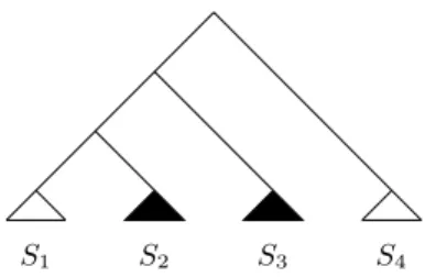
S(L(Fi)) and S(L(Fj)) are not vertex-disjoint in S. Let S′ =S∣L(Fi)∪L(Fj). For example, the simplest case is shown in Figure 5, where the subtrees in white are part of Fi and the ones in black of Fj. In general, a straightforward
check now shows that it is not possible to shrink both T ∣L(Fi) and T ∣L(Fj) to
two distinct single vertices in F′ (one possibly being attached to the ver-tex labeled ρ) by using cherry reductions because to shrink one of the two components to a single vertex it is necessary to cut a subtree of the other component, thereby contradicting that Fi and Fj are both elements in F .
S4
S1 S2 S3
Figure 5: An example of a rooted phylogenetic tree S′ that is used in Case (2) of the proof of Lemma 8 (for details, see text).
Referring back to Figure 5, Fj cannot be shrunk to a single vertex by using
a list of cherry reductions without cutting S1.
Combining both cases establishes the lemma.
Theorem 9. Let S and T be two rooted binary phylogenetic X -trees. Calling allMAAFs(S, T, S, T, k, ∅)
returns all maximum-acyclic-agreement forests for S and T if and only if k ≥ h(S, T ).
Proof. By Lemma 8, each forest that is calculated in the course of execut-ing allMAAFs(S, T, S, T, k, ∅) and checked for acyclicity (see line 5 of the pseudocode of Algorithm 3) is an agreement forest for S and T . Thus, if k ≥ h(S, T ), each forest that is returned from running the algorithm is an acyclic-agreement forest for S and T . Moreover, since k is updated to take advantage of the size of the best solutions that previous recursive calls have found (lines 15, 21, 24 and 34), only maximum-acyclic-agreement forests are returned. It is therefore sufficient to show that each maximum-acyclic-agreement forest for S and T is returned by the algorithm.
Let allMAAFs(S, T, S, T, k, ∅) be a call of Algorithm 3, and, for each l ∈ {1, 2, . . . , h(S, T )+1}, let Glbe the set of all reduced forests of size l that have been computed by executing this call. In other words, Gl precisely contains
all forests that are used as a parameter in a recursive call to allMAAFs in lines 13, 19, 22 and 32 of the pseudocode and, in particular, T ∈ G1.
Furthermore, let F be a maximum-acyclic-agreement forest for S and T . We will prove that, for each l ∈ {1, 2, . . . , h(S, T ) + 1}, the set Gl contains
a reduced forest G′ that is a super-forest for F . This implies that Gh(S,T )+1
contains a reduced forest G′ that is a super-forest of F such that ∣F ∣ = ∣G∣, where G is the underlying forest of G′. Hence, as G and F are both forests for T , it follows that G is isomorphic to F , thereby establishing the theorem. We proceed by induction on l. If l = 1, then the result follows from Ob-servation 1 and because T ∈ G1. Now suppose that the result holds whenever
l ≤ h(S, T ). We will next show that the claim holds for l + 1. Let G′ be a re-duced forest of size l such that G′is a super-forest for F . By the induction as-sumption, G′exists. Let G be the underlying forest of G′. Furthermore, let
∧
Gbe the cherry list that has been used by calling allMAAFs(S, T, S, T, k, ∅) to construct G′, and let R be the phylogenetic tree that is returned from call-ing processCherries*(S, T,
∧
G). Since ∣G∣ < ∣F ∣, it follows from Lemma 7 that R contains a cherry {a, c}. Let L(a) ⊂ X and L(c) ⊂ X be the label sets of the leaf vertices a and c, respectively, in R, and let a′∈ L(a) and c′∈ L(c). Furthermore, if {a, c} is a contradicting cherry for R and G′ and a ∼G′ c, letL(B) ⊂ X be the union of labels of all leaf vertices that are contained in the pendant subtree below eB in G′. Note that, since G′ is a super-forest for
such that L(a) ⊆ L(Fi)and L(c) ⊆ L(Fj). The rest of the proof distinguishes
two cases depending on whether {a, c} is a contradicting or common cherry for R and G′.
First, suppose that {a, c} is a contradicting cherry for R and G′. To derive a contradiction, assume that Gl+1 does not contain any reduced forest that is a super-forest of F . In particular, this implies that deleting any edge associated with {a, c} is a bad choice for G′ and F since no resulting forest is a super-forest for F although they all satisfy Condition (2) in the definition of a super-forest. Thus, one of the following holds:
(1) a ≁G′ c and both edges {ea} and {ec} are bad choices for G′ and F ;
(2) a ∼G′ c and all edges {ea}, {eB} and {ec}are bad choices for G′ and F .
Case (1). Observe that neither G′− {ea}nor G′− {ec}is a super-forest of F . This implies that F does not contain an element Fisuch that L(a) = L(Fi)or L(c) = L(Fi). Thus F contains two distinct components Fj and Fk such that
L(a) ⊂ L(Fj) and L(c) ⊂ L(Fk), and for which there exist elements x, y ∈ X such that x ∈ L(Fj), x ∉ L(a), y ∈ L(Fk), and y ∉ L(c). By construction,
each of x and y is contained in a label of a distinct leaf in R. Now, recalling that {a, c} is a cherry of R, we have that lcaR(a′, c′, x, y) is an ancestor of
lcaR(a′, c′) and, therefore, lcaS(a′, c′, x, y) is an ancestor of lcaS(a′, c′). Fur-thermore, as a′, x ∈ L(Fj) and c′, y ∈ L(Fk), it now follows that S(L(Fj)) and S(L(Fk)) do both have the vertex lcaS(a′, c′) in common; thereby con-tradicting that F is an agreement forest for S and T .
Case (2). Observe that no forest in {G′− {ea}, G′− {eB}, G′− {ec}}is a super-forest of F . This implies that F does not contain any element Fi such that
L(a) = L(Fi) or L(c) = L(Fi) or a subset F′ of F such that L(B) = L(F′). We next consider three subcases.
First, assume that F contains a component Fj such that L(a) ⊂ L(Fj), L(c) ⊂ L(Fj)and there exists at least one element in the intersection L(B) ∩ L(Fj). Let b′ be such an element. By construction, each of a′, b′, and c′
is contained in a label of a distinct leaf in R. Now, recalling that {a, c} is a cherry of R, we have that lcaR(a′, b′, c′) is an ancestor of lcaR(a′, c′) and, therefore, lcaS(a′, b′, c′)is an ancestor of lcaS(a′, c′). On the contrary, let Gk be the element of G′ that contains the leaf labeled L(a) and the leaf labeled L(c). Since Gk also contains a leaf whose label contains b′ and due to the
definition of eB, we have that lcaGk(a
′, b′, c′) is an ancestor of lca Gk(a
′, b′)
or lcaGk(c
′, b′) and, therefore, lca
T(a′, b′, c′) is an ancestor of lcaT(a′, b′) or lcaT(c′, b′). Thus, S∣{a′, b′, c′} ≇T ∣{a′, b′, c′}; thereby contradicting that F is a maximum-acyclic-agreement forest for S and T .
Second, assume that F contains a component Fj such that L(a) ⊂ L(Fj),
L(c) ⊂ L(Fj), and L(B) ∩ L(Fj) = ∅. Then, since there exists no subset F′
of F such that L(B) = L(F′), there exists a distinct element Fk ∈ F such that b′∈ L(Fk)for any b′∈ L(B) and there exists an element x ∈ X for which x ∈ L(Fk) and x ∉ L(B). Let Gk be the element of G′ that contains the leaf labeled L(a). Clearly, Gk also contains the leaf labeled L(c) and the
leaf whose label contains b′. Furthermore, since G is a super-forest for F , note that Gk contains a leaf whose label contains x. Furthermore, by the
definition of eB, we have that the lcaGk(b
labeled a′ to the leaf labeled c′ in Gkand, therefore, the lcaT(b′, x) lies on the
path from the leaf labeled L(a) to the leaf labeled L(c) in T . Now, it is easily checked that Fj and Fk are not vertex-disjoint in T ; thereby contradicting
that F is an agreement forest for S and T .
Third, assume that F contains two components Fj and Fk such that
L(a) ⊂ L(Fj) and L(c) ⊂ L(Fk). Hence, there exist elements x, y ∈ X such that x ∈ L(Fj), x ∉ L(a), y ∈ L(Fk), and y ∉ L(c). Note that x or y may or
may not be elements of L(B). In this case, it is straightforward to see that we can derive the same contradiction as in Case (1).
By combining Cases (1) and (2), we deduce that there exists a super-forest of F that can be constructed from G′ by deleting one of {ea, ec} if a ≁G′ c or one of {ea, eB, ec} if a ∼G′ c. Thus, this super-forest is an element
of Gl+1.
Second, suppose that {a, c} is a common cherry for R and G′. Again, to derive a contradiction, assume that Gl+1 does not contain any reduced forest
that is a super-forest of F . In particular, this implies that ea, ec, and {a, c}
are all bad choices for G′ and F . Thus, similar to Case (1), F contains two distinct components Fj and Fk such that L(a) ⊂ L(Fj) and L(c) ⊂ L(Fk), and for which there exist elements x, y ∈ X such that x ∈ L(Fj), x ∉ L(a),
y ∈ L(Fk), and y ∉ L(c). Applying the same argument as in Case (1), this
con-tradicts the fact that the elements of F are vertex-disjoint in S. Thus, one of ea, ec, or {a, c} is not a bad choice for G′ and F . If eaor ecis not a bad choice
On the other hand, if eaand ec are both bad choices for G′and F , then {a, c}
is not such a choice. Hence, calling cherryReduction(R, G′, M, {a, c}) re-turns a forest G′′that is a super-forest for F . Note that the underlying forest of G′′ is G. Since ∣G∣ < ∣F ∣, it follows from Lemma 7, that after some addi-tional recursions of allMAAFs, the algorithm chooses a cherry in line 10 of the pseudocode of allMAAFs and subsequently deletes an edge in order to obtain a forest of size ∣G∣ + 1. Then by applying the arguments of Cases (1) and (2), and the argument of this paragraph (depending on the type of cherry the algorithm has chosen), it is easily checked that Gl+1 contains a forest that
is a super-forest of F . This completes the proof of the theorem.
5
Running time of the algorithm
In this section, we detail the running time of the algorithm allMAAFs. Theorem 10. Let S and T be two rooted binary phylogenetic X -trees, and let k be an integer.The running time of allMAAFs(S, T, S, T, k, ∅) is O(3∣X ∣). Proof. Let F be a forest for T that has been obtained from T by deleting n edges. Recall that allMAAFs stops when F = ∅ (see Remark 5). It is easy to see that, ∣X ∣ − n − 1 cherry reductions are needed to reduce F to a forest, say F′, such that F′= ∅. Thus, the number of recursive calls is O(∣X ∣). Since allMAAFs is called for at most 3 times from within each recursion, it now follows that the running time of allMAAFs(S, T, R, F, k, M) is O(3∣X ∣)as claimed.
purely theoretical, it can be significantly optimized in the following way. Bordewich and Semple [? ] showed that the problem of calculating the minimum number of hybridization events that is needed to simultaneously explain two rooted binary phylogenetic X -trees S and T is fixed-parameter tractable. They used two reductions – called the subtree and chain reduction – to establish this result. Loosely speaking, these reductions replace different types of features that are common to S and T with a small number of new leaves, thereby shrinking the original trees to their respective cores while preserving their hybridization number in a well-defined way. In fact, these two reductions are sufficient to yield a kernelization of the above-mentioned problem. More precisely, it is shown in [? , Lemma 3.3] that, by repeatedly applying the subtree and chain reductions to S and T until no further reduc-tion is possible, the leaf set size of the so-obtained rooted binary phylogenetic trees is at most 14h(S, T ). It is now straightforward to see that modifying allMAAFs(S, T, R, F , k, M ) in the following way is sufficient to make use of this result.
1. If R = S and F = T , apply the subtree and chain reduction until no further reduction is possible and directly return (∅, k − 1) if the leaf set size of the obtained trees is greater than 14k.
2. Introduce a new global variable, say w, that is used to keep track of the weight of each initially reduced common chain of S and T (for details, see [? ]). Additionally, whenever cherryExpansion is called for a forest throughout a run of allMAAFs, also call subtreeExpansion and chainExpansion to reverse each initially performed subtree and
chain reduction, respectively.
3. For each potential acyclic-agreement forest F′ for S and T that is returned from calling cherryExpansion, subtreeExpansion, and chainExpansion (see line 4 of the pseudocode of allMAAFs), do not only check if F′ is acyclic, but also whether or not it is a so-called legitimate-agreement forest (for details, see [? ]). Note that this additional check can be performed in polynomial time.
We denote this extended version by allMAAFs*(S, T, S, T, k, ∅).
Now, noting that the subtree and chain reduction can be computed in O(n3) for two rooted binary phylogenetic X -trees, where n = ∣X ∣ [? ], the
next corollary is an immediate consequence of Theorem 10, and the kernel-ization ideas that are presented in [? ] and briefly summarized prior to this paragraph.
Corollary 11. Let S and T be two rooted binary phylogenetic X -trees, and let k be an integer.The running time of allMAAFs*(S, T, S, T, k, ∅) is O(314k+
n3), where n = ∣X∣.
We next outline why, despite the theoretical worst-case running time, the practical running time of allMAAFs is quick.
Practical running time An alternative approach to calculating all maximum-acyclic-agreement forests for two rooted binary phylogenetic trees is to delete all possible subsets of edges in the first tree and to check which of the resulting forests are acyclic. If one considers the forests of the first tree by
increasing number of components and stops as soon as one finds an acyclic-agreement forest whose size is greater than the smallest acyclic-acyclic-agreement forest found, this yields an algorithm whose theoretical worst-case running time is less than the worst-case running time of allMAAFs. An algorithm that uses advanced ideas of this approach and calculates one maximum-acyclic-agreement forest was presented in [? ]. However, subsequently to the publication of [? ], two algorithms [? ? ] have been published that outperform the former algorithm for many data sets. Moreover, preliminary results (published in the third author’s Master’s thesis [? ]) indicate that extending the algorithm of [? ] in a way so that it finds all maximum-acyclic-agreement forests results in an algorithm that is slower than allMAAFs in terms of practical running times.
To get an idea why our algorithm in practice performs better than such a naive algorithm having a better worst-case running time, one has to consider the following issues with regards to allMAAFs:
1. Many computational paths of the search tree are not considered in their full depth due to the use of k (this is particularly important if k > h(S, T )) and to the presence of lines 16-17.
2. The theoretical running time presented in Theorem 3 considers the worst-case scenario which is achieved by alternatingly processing con-tradicting and common cherries. The best case scenario, in contrast, is achieved when only contradicting cherries are processed during the first k recursive calls of each search path. Since only forests of size smaller or equal to k are considered, our search tree has at most O(3k)different
leaves in this case and thus, at most O(3k)recursive calls are performed
in total. This means there is a large gap between the worst-case and the best-case running times. By applying the subtree and chain reduction before entering the algorithm one can reduce the number of possible cherries to process what pushes the practical running time towards the running time of the best case scenario.
Nevertheless, if h(S, T ) is sufficiently small, a search and bound approach considering all possible solutions for increasing values of k may be faster than our approach. In summary, we think that the practical running time of allMAAFs is competitive, which may be an important reason for many biologists to use our algorithm in order to analyze their data sets.
6
Discussion
A topical question in current mathematical research on reticulate evolution is how to construct all rooted hybridization networks that display a pair of rooted binary phylogenetic trees such that the number of hybridization ver-tices is minimized. In this paper, we have made a first step towards achieving this goal by developing the first non-naive algorithm—called allMAAFs— that computes all maximum-acyclic-agreement forests for two rooted binary phylogenetic trees on the same taxa set. Furthermore, we have shown that the algorithm presented in [? ], which is freely available as part of Dendro-scope [? ], is correct by providing formal proofs. Despite the theoretical worst-case running time of allMAAFs, the authors of [? ] have shown that it runs quickly for many biological and simulated data sets. At the end of
Section 5 we gave some reasons why the practical running time is good. It is part of ongoing research to extend the algorithm HybridPhylogeny [? ] in order to compute all possible hybridization networks that display a pair of rooted phylogenetic trees and whose number of hybridization vertices is min-imized when a maximum-acyclic-agreement forest for these two trees given. In combination with allMAAFs, such an algorithm will then compute all possible minimum hybridization networks that display a pair of phylogenetic trees.
Acknowledgements
We would like to thank Daniel Huson for helpful discussions and two anony-mous reviewers for their comments. Financial support from the University of T¨ubingen is gratefully acknowledged. This work has been partially funded by the ANCESTROME project ANR-10-IABI-0-01. This publication is the contribution no. 2012-XXX of the Institut des Sciences de l’Evolution de Montpellier (UMR 5554-CNRS-IRD).