HAL Id: hal-00584148
https://hal.archives-ouvertes.fr/hal-00584148v2
Submitted on 1 May 2012
HAL is a multi-disciplinary open access archive for the deposit and dissemination of sci-entific research documents, whether they are pub-lished or not. The documents may come from teaching and research institutions in France or abroad, or from public or private research centers.
L’archive ouverte pluridisciplinaire HAL, est destinée au dépôt et à la diffusion de documents scientifiques de niveau recherche, publiés ou non, émanant des établissements d’enseignement et de recherche français ou étrangers, des laboratoires publics ou privés.
Mutation rate estimates for 110 Y-chromosome STRs
combining population and father-son pair data.
Concetta Burgarella, Miguel Navascués
To cite this version:
Concetta Burgarella, Miguel Navascués. Mutation rate estimates for 110 Y-chromosome STRs com-bining population and father-son pair data.. European Journal of Human Genetics, Nature Publishing Group, 2011, 19 (1), pp.70-5. �10.1038/ejhg.2010.154�. �hal-00584148v2�
Mutation rate estimates for 110 Y-chromosome STRs combining population and
1
father-son pair data
2 3
Concetta Burgarella1,2 & Miguel Navascués1,3* 4
1 CNRS UMR 7625 Écologie et Évolution, École Normale Supérieure, 46 rue d'Ulm
5
75230 Paris (France). 6
2 INIA, Instituto Nacional de Investigación y Tecnología Agraria y Alimentaria. Carretera
7
de La Coruña km 7.5, 28040, Madrid (Spain). 8
3 INRA, UMR CBGP (INRA/IRD/Cirad/Montpellier SupAgro), Campus International de
9
Baillarguet, CS 30016, F-34988 Montferrier-sur-Lez Cedex, France 10
11
* Corresponding author: INRA, UMR CBGP (INRA/IRD/Cirad/Montpellier SupAgro), 12
Campus International de Baillarguet, CS 30016, F-34988 Montferrier-sur-Lez Cedex, 13 France 14 phone: +33(0)4.99.62.33.42 15 fax: +33(0)4.99.62.33.45 16 e-mail: [email protected] 17 18 19 20
Running title: Mutation rate estimates for Y-STRs 21
ABSTRACT 22
23
Y-chromosome microsatellites (Y-STRs) are typically used for kinship analysis and 24
forensic identification as well as for inferences on population history and evolution. All 25
applications would greatly benefit from reliable locus-specific mutation rates, to improve 26
forensic probability calculations and interpretations of diversity data. However, estimates of 27
mutation rate from father-son transmissions are available for few loci and have large 28
confidence intervals, due to the small number of meiosis usually observed. By contrast, 29
population data exist for many more Y-STRs, holding unused information about their 30
mutation rates. To incorporate single locus diversity information into Y-STR mutation rate 31
estimation, we performed a meta-analysis using pedigree data for 80 loci and individual 32
haplotypes for 110 loci, from 29 and 93 published studies respectively. By means of 33
logistic regression we found that relative genetic diversity, motif size and repeat structure 34
explain the variance of observed rates of mutations from meiosis. This model allowed us to 35
predict locus-specific mutation rates (mean predicted mutation rate 2.12×10⁻³, SD = 36
1.58×10⁻³), including estimates for 30 loci lacking meiosis observations and 41 with a 37
previous estimate of zero. These estimates are more accurate than meiosis based estimates 38
when a small number of meiosis is available. We argue that our methodological approach, 39
by taking into account locus diversity, could be also adapted to estimate population or 40
lineage specific mutation rates. Such adjusted estimates would represent valuable 41
information for selecting the most reliable markers for a wide range of applications. 42
Keywords: mutation rate, Y-chromosome microsatellites, meiosis, population genetics,
44
glm 45
INTRODUCTION 46
47
Around four hundred microsatellite markers from the Y human chromosome have been 48
made available to date (e.g.1), with important applications in forensic analyses as well as in 49
genealogy research. However, reliable locus-specific mutation rates are needed to carefully 50
choose loci to minimize the error rate in kinship analysis and sample identification 2 while 51
obtaining the maximum discriminatory power (e.g.3-5). Also in population genetics and
52
evolutionary studies, correct inferences on the timing of major demographic events, the age 53
of the most common ancestor, as well as dating Y-lineages and tracing disease evolution 54
are based on the knowledge of mutation rates (e.g. 6-8). 55
56
Population genetic theory predicts the genetic diversity of loci in function of their mutation 57
rates (µ) and the effective size of populations (N). Therefore, it is possible to obtain 58
estimates of the joint parameter θ=2Nµ from genetic diversity indices. In the case of loci 59
evolving under a stepwise mutation model (SMM, generally assumed for microsatellites) it 60
is possible to use the variance (V) in allele repeat count (i.e. allele size measured in number 61
of repeats) and the ‘homozygosity’ (
∑
= = k i i p H 1 2, where k is the number of different alleles
62
in the population and pi is the frequency of the ith allele; note that the term homozygosity is
63
not biologically meaningful for haploid loci but it will be used through the article for the 64
sake of simplicity) for the estimation of θ using the following relationships 9: 65 V V ˆ ˆ = θ [1] 66
⎟ ⎠ ⎞ ⎜ ⎝ ⎛ − = ˆ1 1 2 1 ˆ 2 H H θ [2] 67
where the hat denotes estimated values. However, because it is difficult to separate the 68
effects of demography (i.e. N), estimates of θ provide little information about mutation rate. 69
Nevertheless, it is possible to obtain information about relative mutation rates. In the case 70
of effective population size being the same among loci within one population (i.e. neutral 71
loci with same ploidy level, such as the Y-STRs), the ratio between the θ of two loci should 72
be the same as the ratio between their mutation rates 10. However, relative mutation rate 73
estimates have limited utility for dating evolutionary events or calculating forensic 74
probabilities. 75
76
Absolute mutation rate estimates can be obtained by the analysis of allele transmissions in 77
pedigrees (e.g. 11,12). The proportion of allele mismatches in father-son transmissions is 78
currently the most widely used approach to obtain estimates of mutation rates for Y-STRs. 79
Because of the low values of mutation rates, large number of father-son pairs must be 80
genotyped to obtain accurate estimates. This has limited the number of Y-STR loci for 81
which these estimates exist and many of them have been obtained from rather low sample 82
sizes. On the other hand, population diversity data exist for many more Y-STRs, holding 83
unused information about their mutation rates. The objective of this work is to present a 84
method to combine pedigree and population data for the estimation of mutation rates and to 85
provide locus-specific mutation rate estimates for 110 Y-STR loci (71 of which had no 86
previous estimate). 87
MATERIALS AND METHODS 89
90
Source of population data
91 92
Population data for 110 Y- chromosome microsatellite loci have been collected from 93 93
published works, for a total of 22,165 individual haplotypes (note that each individual was 94
genotyped for a subset of loci and never for all of them). Locus names, sample sizes and 95
references are detailed in Supplementary table S1. Locus nomenclature and allele call have 96
been thoroughly checked to assure congruence across works and to remove duplicate data. 97
Any population data with incongruent allele codes were either made uniform (when 98
information provided by authors made it possible unequivocally) or excluded from analysis. 99
Specifically, data from GATA H4 and GATA H4.1 have been pooled under the name 100
GATA H4.1 by applying the appropriate correction to allele calls13,14 and DYS389II has 101
been transformed into DYS389B by subtracting allele size of DYS389I15. Multi-copy loci 102
as well as single individuals with duplicated or variant alleles were excluded from the 103
analysis. Data sets were chosen in order to obtain a maximum representation of loci and of 104
geographical areas; collection of data stopped when no additional data sets could be found 105
that would add data for new loci or would increase the order of magnitude of the sample 106
size for individuals genotyped for a locus. 107
108
Source of meiosis (father-son pair) data
109 110
Direct observations of mutation events from meiosis data (father-son pairs) have been 111
collected for 80 loci among the 110 loci with population data, from 29 published studies 112
(table 1 and supplementary table S2). Confidence intervals from binomial probability 113
distribution were estimated according to Wilson method16. Mutations assigned to 114
DYS389II were carefully checked to discriminate those actually occurring in the DYS389I 115
fragment from those occurred in the DYS389B fragment. Discrimination was always 116
possible except for data from reference 11, which were excluded for this locus.
117 118
Statistical analysis
119 120
Population data were analyzed to obtain estimates of relative mutation rates between pairs 121
of loci from allele repeat count variance and homozygosity. The relationship between 122
relative mutation rates and meiosis based mutation rates was assessed by logistic regression 123
using loci with both population and meiosis data. Inferred relationship was then used to 124
predict mutation rates for all loci, including those lacking of meiosis data. Analysis 125
procedure is detailed below. 126
127
First, we selected one locus to serve as reference (i.e. mutation rates for all other loci will 128
be relative to this one). As mentioned above, not all individuals are genotyped for the same 129
set of loci (cf. Supplementary table S1), thus it is not possible to use the whole data set in 130
the logistic regression (although data from unused loci will be useful for predictions, see 131
below). As a consequence, a reference locus has to be chosen in a way to maximize the 132
amount of information used (i.e. to maximize the number of loci with meiosis participating 133
in the regression analysis). In other words, the reference locus has to be the one which 134
shares genotype data with the greatest number of loci with meiosis. To achieve this, we 135
used the following criteria (in this order): (i) there should be meiosis data for the reference 136
locus, (ii) the number of loci with meiosis data (for at least 100 transmissions) and 137
genotyped in individuals (from the population data) also genotyped for the reference locus 138
should be maximum, (iii) the number of loci genotyped in individuals also genotyped for 139
the reference locus should be maximum and (iv) the sampling size (number of individuals 140
from population data) of the reference locus should be maximum. Note that the choice of 141
the reference locus influences only the amount of data used in the analysis. Otherwise, the 142
reference locus only sets an arbitrary scale to the relative mutation rates calculated from 143
genetic diversity indices. 144
145
Relative mutation rate (R=μl μr ) for each locus l was estimated exclusively from
146
individuals genotyped for both locus l and reference locus r. This ensures that the genetic 147
diversity of the sample of both loci has been influenced by the same demographic history 148
(this allows assuming the same effective population sizes). Thus, in the absence of 149
selection, the differences in genetic diversity can be attributed solely to the mutation 150
process. Moreover, because of the complete linkage of Y-STRs, data for both loci will 151
share also the same exact genealogy (even if a selective process was in action). Because 152
both loci have the same genealogy, estimates of the mutation rate ratios will be more 153
accurate than in unlinked loci whose genealogies would vary largely due to the randomness 154
of the coalescent process (e.g. nuclear STRs compared in reference17 ). Estimates θˆV ,l, θˆV ,r,
l H ,
ˆ
θ and θˆH ,r were obtained from repeat count variance and homozygosity for loci l and r
156
(using equations 1 and 2) and two estimates of the relative mutation rate were calculated 157
from ratios RˆV =θˆV,l θˆV,r and RˆH =θˆH,l θˆH,r .
158 159
A number of loci (24 out of 110, see supplementary table S1) for which there is population 160
data available, were not genotyped at the reference locus in any of the samples. For those 161
loci, relative mutation rates were estimated as described above but using the total number 162
of individuals available for each locus (we will denote these estimates R'ˆV and R'ˆ ). It H
163
must be noted that R'ˆV and R'ˆ might have a larger error than H RˆV and Rˆ because the H
164
effects of demography are more loosely accounted for. For this reason they were not used 165
for the estimation of the logistic regression model but only in the prediction of mutation 166
rates (see details below). 167
168
A generalized linear model (binary logistic regression18) was applied to the proportion of
169
mutations per meiosis. We tested for the relationship between meiosis mutation rate and 170
population relative mutation rates (RˆV,Rˆ ). Besides, some studies have proposed that H
171
microsatellite mutation rates depend on allele length19,20, motif size and motif structure19. 172
Thus, in addition to RˆV and Rˆ , mean allele repeat count (A; estimated from the H
173
population data), CG content in motif (PCG; proportion of CG base pairs in the motif), and
174
the categorical variables motif size (M; tri-, tetra-, penta- or hexanucleotide motif) and 175
repeat structure (S; simple versus complex) were considered explanatory variables. 176
Information about Y-STR motifs was obtained from21-24.
177 178
Problems of multicollinearity were evaluated on the full model (containing all explanatory 179
variables), as collinear variables represent partial redundant information and correlations 180
between variables generate unreliable individual estimates of regression coefficients. 181
Alternative models obtained after removing different combinations of collinear variables 182
were considered and reduced by stepwise removal of variables to minimize Akaike 183
information criterion (AIC, i.e. a standard procedure to find the explanatory variable 184
combination which accounts for the maximum of the variability with the minimum number 185
of variables). Reduced models were hereafter compared through their pseudo-R2 value 186
(calculated by the maximum likelihood method25). Pseudo-R2 measures the amount of
187
variation in the observed mutation rates explained by the model. The reduced model with 188
the highest pseudo-R2 was chosen to predict mutation rates for all loci. As explained before, 189
for loci whose RˆV and Rˆ could not be calculated, H R'ˆV or R'ˆ were used as a proxy H
190
(estimates for those loci will be distinguished in the results, as they are theoretically less 191
reliable). 192
193
All statistical analyses were performed in R26, using packages binom27 for calculation of 194
confidence intervals (CI), ape28 for calculation of heterozygosity, and pscl29 for calculation 195
of pseudo-R2. A script in R language with the detailed analysis is available from the authors 196
upon request. 197
198
Validation of the approach
199 200
Performance of the statistical approach proposed was evaluated by means of simulations. In 201
each simulation a set of 108 fully linked loci were considered. Loci were divided in three 202
motif size categories: 36 ‘tri’, 36 ‘penta’ and 36 ‘tetra’. ‘Tri’ loci evolved at six different 203
mutation rates (10-4, 2×10⁻⁴, 4×10⁻⁴, 8×10⁻⁴, 1.6×10⁻³ and 3.2×10⁻³, measured in mutations
204
per generation). ‘Penta’ loci evolved at mutation rates double to those for ‘tri’ loci (i.e. 205
2×10⁻⁴, 4×10⁻⁴, 8×10⁻⁴, 1.6×10⁻³, 3.2×10⁻³ and 6.4×10⁻³) and ‘tetra’ loci evolved at mutation 206
rates quadruple to those for ‘tri’ loci (i.e. 4×10⁻⁴, 8×10⁻⁴, 1.6×10⁻³, 3.2×10⁻³, 6.4×10⁻³ and 207
1.28×10⁻²). Note that categories ‘tri’, ‘penta’ and ‘tetra’ are arbitrary (both in their name 208
and their influence in mutation rate) and are only used to include the effect of a categorical 209
variable in the evaluation of the proposed approach. For each mutation rate within each 210
locus category, six loci differing in the amount of observed meiosis (i.e. 50, 150, 500, 1500, 211
5000 and 15000 meiosis) have been considered. To sum up, tree categories times six 212
mutation rates, times six loci differing in the number of meiosis gives 108 total simulated 213
loci. 214
215
Meiosis were simulated using the binomial distribution, with the probability equal to the 216
true mutation rate and the number of observations to the number of meiosis. Population 217
data were simulated with the coalescent simulator SimCoal2 30 under a stepwise mutation 218
model. A sample size of 500 haplotypes was taken from a single population of constant 219
effective size of 1500 individuals (this effective size combined with the simulated mutation 220
rates yielded genetic diversity levels similar to those found on Y-STRs, i.e. around 2-14 221
alleles per locus). 222
223
Mutation rates estimates were obtained for each locus either by using exclusively meiosis 224
data or by using a logistic regression on the observed mutations in meiosis using Rˆ and H
225
the simulated categorical variable ('motif size') as explanatory variables, according to the 226
final model chosen with the real data (see results). The process was repeated 10000 times. 227
Root of the relative mean squared error (
∑
(
)
= − = n i i n RrelMSE 1 2 2 ˆ 1 μ μ μ , where n is the 228number of simulations, μˆ is the estimated mutation rate in simulation i and µ is the true i
229
mutation rate) was calculated for the two types of mutation rate estimates at each of the 108 230 loci. 231 232 RESULTS 233 234
Locus DYS643 was selected as reference locus following the criteria described above. 235
Mutation rates relative to reference locus were estimated from repeat count variance and 236
homozygosity for 86 loci, which were used in the logistic regression model (Table 1). 237
Problems of multicollinearity were found between RˆVand the mean repeat count (A),
238
betweenRˆ and A and betweenH Rˆ CG content in motif (PH CG). Thus, we considered three
239
alternative models with a different combinations of non-collinear variables each: model m1 240
including Rˆ plus the motif size (M) and repeat structure (S); model m2 including H RˆV plus
M, content in motif (PCG) and S; m3 including A plus M, PCG and S. The AIC minimization
242
approach led to the removal of variable PCG in m2 and m3. Final models (supplementary
243
tables S3, S4 and S5) were ranked by their pseudo-R2 values: 0.84 for reduced m1, 0.83 for 244
reduced m2, and 0.67 for reduced m3. Reduced m1 model was therefore selected to make 245
predictions on mutation rates from population data for all loci, using Rˆ or H R'ˆ . Reduced H
246
m1 (Lµ = β0 + β1Rˆ + βH 2Mtri + β3Mtetra + β4Mpenta + β5Ssimple + error; table S3 and figure 1)
247
shows that mutation rate estimated from meiosis (Lµ) increases with Rˆ (i.e. βH 1>0),
248
depends on repeat size (highest for tetranucleotide loci followed by penta- and tri-, i.e. β3>
249
β4> β2 ), and on the complexity of the loci (higher for simple than for complex loci, i.e.
250
β5>0). Note that the coefficient of categorical variables is a value relative to the coefficient
251
of the category no explicitly represented in the equation (i.e. hexanucleotide repeat motif 252
class and the complex structure class). 253
For comparison, results from simple models (i.e. including each explanatory variable 254
separately) are reported in supplementary table S6. They show that all explanatory 255
variables, but the repeat structure, explain significantly part of the variability of mutation 256
rate estimates, although during the model minimization process some were excluded 257
because they provide redundant or non-independent information. Although repeat structure 258
is not able to significantly explain mutation rate variability when it is the only explanatory 259
variable, it is found to provide significant information when analyzed in combination with 260
other explanatory variables (supplementary tables S3, S4 and S5). 261
Predicted values for mutation rates range from 3.60×10⁻⁴ mutations per generation for 263
DYS645 to 9.64×10⁻³ for DYS449 (average 2.12×10⁻³, SD = 1.58×10⁻³; table 1). For those
264
loci which are not genotyped in any individual genotyped for the reference locus in the 265
population data (see table 1), differences in population history and genealogies are expected 266
to make an additional contribution to the variance in mutation rate estimates, although this 267
does not seem to be too important (exclusion of those loci hardly changes the average 268
predicted mutation rate, to 2.25×10⁻³, SD = 1.65×10⁻³). In total, regression approach
269
provides an estimate for 71 loci with either zero observed mutations in meiosis (i.e. point 270
estimate of mutation rate was zero) or lacking meiosis observations. 271
272
It is worth to notice that 45 out of 80 loci with meiosis data share their meiosis mutation 273
rate estimates and CI with at least another locus (given that often the same number of 274
mutations are observed in the same number of meiosis), while mutation rates predicted by 275
regression are different from each other for all loci. Simulations showed that the error 276
associated to meiosis mutation rate estimates is strongly influenced by the number of 277
meiosis, while the error of regression estimates seems independent of the number of 278
observed meiosis (figure 2 reports results for the four simulated mutation rates shared by all 279
loci categories, see methods). Error in both estimates depends on the true mutation rate, 280
decreasing for higher true mutation rates. However, this decrease is stronger for regression 281
estimates than for meiosis estimates. An interesting feature is that regression estimates are 282
more accurate than meiosis estimates when a low number of meiosis is available, but the 283
contrary occurs for high number of meiosis observations. Although this general pattern 284
seems to be independent of the true mutation rate, the threshold from which meiosis 285
estimates are more accurate than regression estimates increases with the true mutation rate. 286
It is important to remember that the behaviour described by simulations regards only loci 287
for which a meiosis estimate is available, however the regression approach provides an 288
estimate even when meiosis data are not available. 289
290
DISCUSSION 291
292
Mutation rates are expected to vary substantially across Y- microsatellite loci (reference 31 293
and references therein). Such large variation has been attributed to motif size, complexity 294
of repeat structure and allele size (e.g.12,21,32-34). Our results are in general agreement with 295
the aforementioned works. We found that meiosis mutation rates are positively correlated 296
with population diversity (estimated by either homozygosity or relative repeat count 297
variance, tables S3 and S4), and mean repeat count (table S5), and depends on repeat motif 298
and repeat structure (table S3). The model selection approach used in this work indicates 299
that a model including relative genetic diversity (from homozygosity), repeat motif and 300
repeat structure as predictive variables is the best one to explain the variability found in 301
meiosis based estimates of mutation rate. However, it should be noted that the alternative 302
models tested (table S4 and S5) are valid too, although their lower pseudo-R2 values 303
indicate that they might have a lower performance for making inferences. 304
305
Correlation between mutation rates from meiosis and the relative mutation rates based on 306
homozygosity was positive and highly significant (tables S3 and S6). The latter is estimated 307
from population data, thus corresponds to the “evolutionary” mutation rates (i.e. the 308
effective mutation rate integrated over the history or gene tree of the sample). Pedigree 309
based mutation rate estimates have been shown to be up to 10-fold higher than evolutionary 310
mutation rate estimates (for sequence data), not only in Y-chromosomes (e.g.31,35) but also 311
in mitochondrial loci (e.g.36,37). The reasons for this discrepancy are still under discussion 312
and are likely to be found in the different temporal scale of estimation. In fact, slowly 313
mutating loci or reverse mutations as well as demographic fluctuations or differential 314
selection over generations are expected to affect population based diversity (see discussion 315
in reference 31). It must be noted that our reported estimates (predicted from the logistic 316
model) correspond to the point estimates of mutation rates (i.e. mutation occurrence in 317
single generation). 318
319
Tri-, tetra- and pentanucleotide classes are well represented in the analyzed locus set (with 320
17, 55 and 7 loci respectively), while hexanucleotide class did not contribute much to the 321
regression model because it is present with only one locus (DYS448) with meiosis 322
observations. We found that the value for the model coefficient (β) is much lower for tri- 323
and pentanucleotide loci than for tetranucleotide loci (tables S3 and S4), which corresponds 324
to general lower mutation rates for tri- and pentanucleotide loci than for tetranucleotide loci 325
(table 1). Such a different behaviour is congruent with the results of previous studies. Järve 326
et al.22 recently showed that pentanucleotide markers have two times lower repeat variance 327
and diversity than tetranucleotide markers, a feature probably related to a lower occurrence 328
of replication slippage with longer repeats. Regarding trinucleotide markers, Kayser et al.21 329
found they had often lower variance than tetranucleotide markers, probably because of the 330
effect of low absolute repeat allele lengths included in their sample21. Lower mutability of 331
shorter alleles compared with longer ones has been observed several times32,33,12,34. 332
Accordingly, our results show that the variation in meiosis mutation rates could be 333
significantly explained by mean repeat count (tables S5 and S6). Furthermore, when no 334
diversity variable is included in the model, both repeat count and repeat motif contribute 335
independently to explain the mutation rate variability (i.e. model m3, table S5). 336
337
The repeat structure explains very little the observed STR mutation rates (table S3), but it is 338
maintained after model reduction using the AIC. However, the coefficient β for simple loci 339
is positive in the final reduced m1 (table S3), while it is negative when the repeat structure 340
is used as the only explanatory variable (table S6). Thus, the effect of the repeat structure 341
on mutation rate is of difficult interpretation. Previous studies have failed to find a 342
relationship of simple versus complex repeats with genetic diversity among loci38,32,22. These
343
results might be due to the lack of effect of repeat structure. However, our qualitative 344
classification of loci as ‘simple’ or ‘complex’ could be missing essential information of 345
complex loci (i.e. differential length of the homogeneous array or combination of variable 346
and constant repeats 21) affecting the mutation rate. More precise definitions of the degree
347
of complexity, similar to those used in ref. 21, could yield different results, but require
348
detailed information on loci not readily available. 349
350
The model considered in this work for microsatellite evolution (SMM) predicts single-351
repeat-unit mutational changes. However, violations of this assumption have been reported 352
both in phylogenetic and meiosis studies (e.g.33,34,38,39), suggesting that more complex
353
models than SMM would better explain microsatellite variation. The ratio of variances in 354
number of repeats between two loci can be still considered a good estimator of the ratio of 355
mutation rates even in case of multi-step mutations, provided that deviation from the SMM 356
is similar for both loci (cf. equation 2 in reference17). Although the same argument is not 357
strictly valid for the estimate of θ from homozygosity, small deviations from the SMM 358
change very little the expected homozygosity (cf. Table I from 9). Only 14 mutations (3.1% 359
of total) involving multiple repeat units are included in meiosis data; therefore, SMM can 360
be considered a reasonable approximation. In addition, the great congruence in prediction 361
between models m1 (using homozygosity) and m2 (using repeat count variance) suggests 362
that the mutation model violation is not an issue for the analysis (results not shown). 363
364
Some important outcomes derive from the approach proposed, emphasizing the positive 365
impact of including population polymorphism data for the improvement of mutation rate 366
estimates and the identification of loci distinctiveness. First, mutation rate estimates were 367
obtained for 30 loci lacking estimates from meiosis observations. Second, locus-specific 368
values of mutation rates can be obtained, while meiosis-based estimates give often equal 369
values for several loci. Third, estimates can be obtained also for loci with very low 370
mutation rates, for which a large sample of meiosis data is required to obtain a non-zero 371
mutation rate estimate. Regarding this point, this work provides mutation rate estimates for 372
41 loci whose mutation rate estimate from meiosis was zero because no mutations had been 373
observed. Lastly, regression based estimates present lower error than estimates from 374
meiosis when only a ‘low’ number of meiosis is observed. 375
The analysis performed in this work represents a valuable tool for selecting most reliable 377
markers to increase Y-STR set currently applied in forensic and kinship analyses. Also, the 378
choice of adequate mutation rates keeps being an issue of great concern when inferences on 379
human diversity and population history are pursued, as put in evidence in a recent work6. 380
To account for the different variability of microsatellite loci, these authors use repeat count 381
variance to obtain recalibrated evolutionary mutation rates for groups of loci. Our 382
approximation allows more detailed results by achieving an adjusted mutation rate for each 383
locus separately. The same methodology could be used to estimate population or lineage 384
specific mutation rates, since different lineages and populations are often characterized by 385
specific allele combinations 32,33,39 and mutation rate seems to be affected by allele size and 386
structure. Finally, the analysis presented here can be easily automated for a data base, 387
allowing the updating of estimates when new population and meiosis data are incorporated 388
from upcoming studies. 389 390 391 AKNOWLEDGMENTS 392 393
We wish to thank Frantz Depaulis for his support and suggestions and Joaquín Navascués 394
for its critical review of the manuscript. Two anonymous reviewers have contributed to 395
improve the manuscript. This work was developed during a postdoctoral stay of CB 396
(Bourse pour chercheurs étrangers de la Marie de Paris 2007). 397
398 399
CONFLICT OF INTEREST STATEMENT 400
401
The authors declare no conflict of interest. 402
403 404
Supplementary information is available at European Journal of Human Genetics’ website 405 http://www.nature.com/ejhg/index.html 406 407 408 REFERENCES 409 410
1. Hanson EK, Ballantyne J. Comprehensive annotated STR physical map of the human Y 411
chromosome: Forensic implications. Leg. Med. 2006;8(2):110–120. 412
413
2. Kayser M, Sajantila A. Mutations at Y-STR loci: implications for paternity testing and 414
forensic analysis. Forensic Sci. Int. 2001;118(2–3):116–121. 415
416
3. Mulero JJ, Chang CW, Calandro LM, et al. Development and Validation of the 417
AmpFℓSTR® Yfiler™ PCR Amplification Kit: A Male Specific, Single Amplification 17 418
Y-STR Multiplex System. J. For. Sci. 2006;51(1):64–75. 419
420
4. Lim S, Xue Y, Parkin E, Tyler-Smith C. Variation of 52 new Y-STR loci in the Y 421
Chromosome Consortium worldwide panel of 76 diverse individuals. Int. J. Legal Med. 422
2007;121(2):124–127. 423
424
5. Vermeulen M, Wollstein A, van der Gaag K, et al. Improving global and regional 425
resolution of male lineage differentiation by simple single-copy Y-chromosomal short 426
tandem repeat polymorphisms. Forensic Sci. Int.: Genet. 2009;3(4):205–213. 427
428
6. Shi W, Ayub Q, Vermeulen M, et al. A worldwide survey of human male demographic 429
history based on Y-SNP and Y-STR data from the HGDP-CEPH populations. Mol Biol 430
Evol. 2009:msp243.
431 432
7. Zerjal T, Wells RS, Yuldasheva N, Ruzibakiev R, Tyler-Smith C. A Genetic Landscape 433
Reshaped by Recent Events: Y-Chromosomal Insights into Central Asia. Am. J. Hum. 434
Genet. 2002;71(3):466-482.
435 436
8. Xue Y, Zerjal T, Bao W, et al. Male Demography in East Asia: A North-South Contrast 437
in Human Population Expansion Times. Genetics. 2006;172(4):2431-2439. 438
439
9. Kimmel M, Chakraborty R. Measures of variation at DNA repeat loci under a general 440
stepwise mutation model. Theor. Popul. Biol. 1996;50(3):345–367. 441
442
10. Xu H, Fu Y. Estimating effective population size or mutation rate with microsatellites. 443
Genetics. 2004;166(1):555–563.
444 445
11. Heyer E, Puymirat J, Dieltjes P, Bakker E, de Knijff P. Estimating Y chromosome 446
specific microsatellite mutation frequencies using deep rooting pedigrees. Hum. Mol. 447
Genet. 1997;6(5):799–803.
448 449
12. Gusmão L, Sánchez-Diz P, Calafell F, et al. Mutation rates at Y chromosome specific 450
microsatellites. Hum. Mutat. 2005;26(6):520–528. 451
452
13. Gusmão L, Alves C, Beleza S, Amorim A. Forensic evaluation and population data on 453
the new Y-STRs DYS434, DYS437, DYS438, DYS439 and GATA A10. Int. J. Legal Med. 454
2002;116(3):139–147. 455
456
14. Mulero JJ, Budowle B, Butler JM, Gusmão L. Nomenclature and allele repeat structure 457
update for the Y-STR locus GATA H4. J. For. Sci. 2006;51(3):694–694. 458
459
15. Butler JM, Reeder DJ. Short Tandem Repeat DNA Internet DataBase. 2009. Available 460
at: http://www.cstl.nist.gov/strbase/. 461
462
16. Wilson EB. Probable inference, the law of succession, and statistical inference. J. Am. 463
Stat. Assoc. 1927;22(158):209-212.
464 465
17. Chakraborty R, Kimmel M, Stivers D, Davison L, Deka R. Relative mutation rates at 466
di-, tri-, and tetranucleotide microsatellite loci. Proceedings of the National Academy of 467
Sciences of the United States of America. 1997;94(3):1041-1046.
468 469
18. Hosmer DW, Lemeshow S. Applied Logistic Regression. 2nd ed. New York: 470
Chichester, Wiley.; 2000. 471
472
19. Brinkmann B, Klintschar M, Neuhuber F, Hühne J, Rolf B. Mutation rate in human 473
microsatellites: influence of the structure and length of the tandem repeat. Am. J. Hum. 474
Genet. 1998;62(6):1408–1415.
475 476
20. Ellegren H. Heterogeneous mutation processes in human microsatellite DNA 477
sequences. Nat. Genet. 2000;24(4):400–402. 478
479
21. Kayser M, Kittler R, Erler A, et al. A Comprehensive Survey of Human Y-480
Chromosomal Microsatellites. Am. J. Hum. Genet. 2004;74(6):1183-1197. 481
482
22. Järve M, Zhivotovsky LA, Rootsi S, et al. Decreased Rate of Evolution in Y 483
Chromosome STR Loci of Increased Size of the Repeat Unit. PLoS ONE. 2009;4(9):e7276. 484
485
23. Gusmão L, Butler JM, Carracedo A, et al. DNA Commission of the International 486
Society of Forensic Genetics (ISFG): An update of the recommendations on the use of Y-487
STRs in forensic analysis. Forensic Sci. Int. 2006;157(2–3):187–197. 488
489
24. Leat N, Ehrenreich L, Benjeddou M, Cloete K, Davison S. Properties of novel and 490
widely studied Y-STR loci in three South African populations. Forensic Sci. Int. 491
2007;168(2–3):154–161. 492
493
25. Long JS. Regression Models for Categorical and Limited Dependent Variables. 494
Thousand Oaks, California, USA: Sage Publications, Inc; 1997:297. 495
496
26. R Development Core Team. R: A Language and Environment for Statistical 497
Computing. Vienna, Austria: R Foundation for Statistical Computing; 2009. Available at:
498
http://www.R-project.org. 499
500
27. Dorai-Raj S. binom: binomial confidence intervals for several parameterizations 501
(version 1.0-5). 2009. 502
503
28. Paradis E, Claude J, Strimmer K. APE: analyses of phylogenetics and evolution in R 504
language. Bioinformatics. 2004;20(2):289–290. 505
506
29. Jackman S. pscl: Classes and Methods for R Developed in the Political Science 507
Computational Laboratory, Stanford University. Stanford, California: Department of
508
Political Science, Stanford University; 2008. Available at: http://pscl.stanford.edu/. 509
510
30. Laval G, Excoffier L. SIMCOAL 2.0: a program to simulate genomic diversity over 511
large recombining regions in a subdivided population with a complex history. 512
Bioinformatics. 2004;20(15):2485–2487.
513 514
31. Zhivotovsky LA, Underhill PA, Cinnio lu C, et al. The Effective Mutation Rate at Y 515
Chromosome Short Tandem Repeats, with Application to Human Population-Divergence 516
Time. Am J Hum Genet. 2004;74(1):50–61. 517
518
32. Carvalho-Silva DR, Santos FR, Hutz MH, Salzano FM, Pena SD. Divergent Human Y-519
Chromosome Microsatellite Evolution Rates. J. Mol. Evol. 1999;49(2):204-214. 520
33. Dupuy BM, Stenersen M, Egeland T, Olaisen B. Y-chromosomal microsatellite 522
mutation rates: differences in mutation rate between and within loci. Hum. Mutat. 523
2004;23(2):117–124. 524
525
34. Ge J, Budowle B, Aranda XG, et al. Mutation rates at Y chromosome short tandem 526
repeats in Texas populations. Forensic Sci. Int.: Genet. 2009;3(3):179–184. 527
528
35. Forster P, Röhl A, Lünnemann P, et al. A Short Tandem Repeat-Based Phylogeny for 529
the Human Y Chromosome. American Journal of Human Genetics. 2000;67(1):182–196. 530
531
36. Macaulay VA, Richards MB, Forster P, et al. mtDNA Mutation Rates-No Need to 532
Panic. Am. J. Hum. Genet. 1997;61(4):983-986. 533
534
37. Heyer E, Zietkiewicz E, Rochowski A, et al. Phylogenetic and Familial Estimates of 535
Mitochondrial Substitution Rates: Study of Control Region Mutations in Deep-Rooting 536
Pedigrees. Am. J. Hum. Genet. 2001;69(5):1113-1126. 537
538
38. Forster P, Kayser M, Meyer E, et al. Phylogenetic resolution of complex mutational 539
features at Y-STR DYS390 in aboriginal Australians and Papuans. Mol. Biol. Evol. 540
1998;15(9):1108–1114. 541
542
39. Nebel A, Filon D, Hohoff C, et al. Haplogroup-specific deviation from the stepwise 543
mutation model at the microsatellite loci DYS388 and DYS392. Eur. J. Hum. Genet. 544
2001;9:22–26. 545
Figure 1. Mutation rate estimates (measured in mutations per generation) from meiosis for
546
80 Y-STR loci (points) and prediction from logistic regression for the eight categories of 547
loci defined by motif size and repeat structure (lines). Continuous lines represent the 548
predictions for loci with a simple repeat structure and dashed lines for complex loci. Thick 549
black lines are used for the predictions of tetranucleotide loci, thick grey lines for hexa- 550
loci, thin black lines for penta- loci and thin grey lines for tri- loci. The logistic regression 551
model (Lµ = - 6.863 + 0.539Rˆ - 1.176MH tri + 0.478Mtetra - 1.130Mpenta + 0.236Ssimple +
552
error, see supplementary table S3 for coefficient p-values) gives the relationship between 553
the logit of mutation rate (Lµ) and the predictive variables Rˆ (population relative H
554
mutation rate estimated using homozigosity), M (motif size: tri-, tetra-, penta- and 555
hexanucleotide classes) and S (repeat structure: simple or complex). The model shows that 556
Lµ increases with R ˆ H and depends on repeat size (highest for tetranucleotide loci followed 557
by hexa-, penta- and tri- in this order) and on the complexity of the loci (higher for simple 558
than for complex loci). 559
560
Figure 2. Root of the relative mean squared error (RrelMSE) for mutation rate estimates
561
calculated from meiosis data (filled circles) or from population data (open circles, triangles 562
and squares) at each of 108 simulated loci. RrelMSE for estimates for loci mutating at true 563
mutation rates of (a) 4×10⁻⁴ mutations per generation, (b) 8×10⁻⁴, (c) 1.6×10⁻³ and (d) 564
3.2×10⁻³. RrelMSE for regression based estimates also depends on the category the loci
565
belong to: ‘tri’ (triangles), ‘tetra’ (squares) or ‘penta’ (open circles). 566
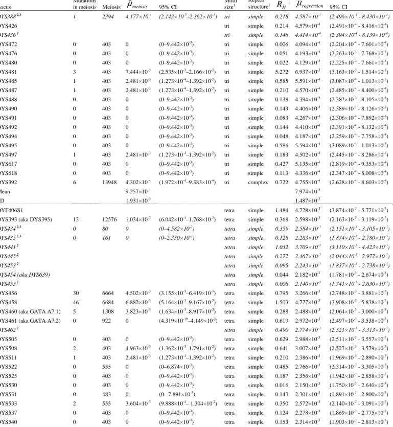
Table 1. Mutation rate estimates (measured in mutations per generation), obtained from
568
combined meiosis data from 29 published studies (listed in supplementary table S2) and 569
predicted from the logistic model, for 110 Y-STR loci. 570
571 572
0.0 0.5 1.0 1.5 2.0 0.000 0.001 0.002 0.003 0.004 0.005 0.006 R^H m utation r ate
tetra− & simple
tetra− & complex
hexa− & simple
hexa− & complex
penta− & simple
penta− & complex
tri− & simple
tri− & complex
● ● ● ● ● ● ● ●
meiosis estimate (tri−) meiosis estimate (tetra−) meiosis estimate (penta−) meiosis estimate (hexa−)
● ● ● ● ● ● ● 50 100 200 500 1000 2000 5000 10000 0.1 0.2 0.5 1.0 2.0 5.0 number of meiosis R re lMSE ● ● ● ● ● ● µ = 4 × 10⁻⁴ a ● ● ● ● ● ● 50 100 200 500 1000 2000 5000 10000 0.1 0.2 0.5 1.0 2.0 5.0 number of meiosis R re lMSE ● ● ● ● ● ● µ = 8 × 10⁻⁴ b ● ● ● ● ● ● 50 100 200 500 1000 2000 5000 10000 0.1 0.2 0.5 1.0 2.0 5.0 number of meiosis R re lMSE ● ● ● ● ● ● µ = 1.6 × 10⁻³ c ● ● ● ● ● ● 50 100 200 500 1000 2000 5000 10000 0.1 0.2 0.5 1.0 2.0 5.0 number of meiosis R re lMSE ● ● ● ● ● ● µ = 3.2 × 10⁻³ d ● ●
estimates from meiosis (all) estimates from regression (tri) estimates from regression (tetra) estimates from regression (penta)
Table 1. Mutation rate estimates (measured in mutations per generation), obtained from combined meiosis data from 29 published studies (listed in supplementary table S2) and predicted from the logistic model, for 110 Y-STR loci.
Locus
Mutations
in meiosis Meiosis μˆmeiosis 95% CI
Motif size1 Repeat structure1 H Rˆ 1 regression μˆ 95% CI DYS388 2,3 1 2394 4.177×10⁻⁴ (2.143×10⁻⁵ –2.362×10⁻³ ) tri simple 0.218 4.587×10⁻⁴ (2.496×10⁻⁴ - 8.430×10⁻⁴ )
DYS426 tri simple 0.214 4.579×10⁻⁴
(2.491×10⁻⁴ - 8.416×10⁻⁴ ) DYS436 2 tri simple 0.146 4.414×10⁻⁴ (2.394×10⁻⁴ - 8.139×10⁻⁴ ) DYS472 0 403 0 (0–9.442×10⁻³ ) tri simple 0.006 4.094×10⁻⁴ (2.204×10⁻⁴ - 7.601×10⁻⁴ ) DYS476 0 403 0 (0–9.442×10⁻³ ) tri simple 0.051 4.193×10⁻⁴ (2.263×10⁻⁴ - 7.768×10⁻⁴ ) DYS480 0 403 0 (0–9.442×10⁻³ ) tri simple 0.022 4.129×10⁻⁴ (2.225×10⁻⁴ - 7.661×10⁻⁴ ) DYS481 3 403 7.444×10⁻³ (2.535×10⁻³ –2.166×10⁻² ) tri simple 5.272 6.937×10⁻³ (3.163×10⁻³ - 1.514×10⁻² ) DYS485 1 403 2.481×10⁻³ (1.273×10⁻⁴ –1.392×10⁻² ) tri simple 0.585 5.591×10⁻⁴ (3.087×10⁻⁴ - 1.013×10⁻³ ) DYS487 1 403 2.481×10⁻³ (1.273×10⁻⁴ –1.392×10⁻² ) tri simple 0.210 4.570×10⁻⁴ (2.485×10⁻⁴ - 8.400×10⁻⁴ ) DYS488 0 403 0 (0–9.442×10⁻³ ) tri simple 0.138 4.394×10⁻⁴ (2.382×10⁻⁴ - 8.105×10⁻⁴ ) DYS490 0 403 0 (0–9.442×10⁻³ ) tri simple 0.143 4.406×10⁻⁴ (2.389×10⁻⁴ - 8.126×10⁻⁴ ) DYS491 0 403 0 (0–9.442×10⁻³ ) tri simple 0.083 4.267×10⁻⁴ (2.306×10⁻⁴ - 7.892×10⁻⁴ ) DYS492 0 403 0 (0–9.442×10⁻³ ) tri simple 0.144 4.410×10⁻⁴ (2.391×10⁻⁴ - 8.132×10⁻⁴ ) DYS494 0 403 0 (0–9.442×10⁻³ ) tri simple 0.048 4.187×10⁻⁴ (2.259×10⁻⁴ - 7.758×10⁻⁴ ) DYS495 0 403 0 (0–9.442×10⁻³ ) tri simple 0.586 5.594×10⁻⁴ (3.089×10⁻⁴ - 1.013×10⁻³ ) DYS497 1 403 2.481×10⁻³ (1.273×10⁻⁴ –1.392×10⁻² ) tri simple 0.183 4.502×10⁻⁴ (2.445×10⁻⁴ - 8.286×10⁻⁴ ) DYS617 0 403 0 (0–9.442×10⁻³ ) tri simple 0.427 5.135×10⁻⁴ (2.819×10⁻⁴ - 9.353×10⁻⁴ ) DYS618 0 403 0 (0–9.442×10⁻³ ) tri simple 0.113 4.336×10⁻⁴ (2.347×10⁻⁴ - 8.008×10⁻⁴ ) DYS392 6 13948 4.302×10⁻⁴ (1.972×10⁻⁴ –9.383×10⁻⁴ ) tri complex 0.722 4.755×10⁻⁴ (2.628×10⁻⁴ - 8.603×10⁻⁴ ) Mean 9.257×10⁻⁴ 7.974×10⁻⁴ SD 1.931×10⁻³ 1.487×10⁻³
DYF406S1 tetra simple 1.484 4.728×10⁻³
(3.874×10⁻³
- 5.771×10⁻³
) DYS393 (aka DYS395) 13 12576 1.034×10⁻³
(6.042×10⁻⁴ –1.768×10⁻³ ) tetra simple 0.368 2.598×10⁻³ (2.163×10⁻³ - 3.119×10⁻³ ) DYS434 2,3 0 80 0 (0–4.582×10⁻² ) tetra simple 0.359 2.584×10⁻³ (2.151×10⁻³ - 3.105×10⁻³ ) DYS435 2,3 0 161 0 (0–2.330×10⁻² ) tetra simple 0.128 2.283×10⁻³ (1.874×10⁻³ - 2.780×10⁻³ ) DYS441 2 tetra simple 1.032 3.709×10⁻³ (3.110×10⁻³ - 4.423×10⁻³ ) DYS445 2 tetra simple 0.272 2.467×10⁻³ (2.044×10⁻³ - 2.977×10⁻³ ) DYS453 2 tetra simple 0.095 2.243×10⁻³ (1.837×10⁻³ - 2.738×10⁻³ ) DYS454 (aka DYS639) tetra simple 0.044 2.182×10⁻³
(1.781×10⁻³ - 2.674×10⁻³ ) DYS455 2 tetra simple 0.008 2.140×10⁻³ (1.741×10⁻³ - 2.630×10⁻³ ) DYS456 30 6664 4.502×10⁻³ (3.155×10⁻³ –6.419×10⁻³ ) tetra simple 0.795 3.266×10⁻³ (2.748×10⁻³ - 3.881×10⁻³ ) DYS458 46 6684 6.882×10⁻³ (5.164×10⁻³ –9.167×10⁻³ ) tetra simple 1.503 4.777×10⁻³ (3.908×10⁻³ - 5.838×10⁻³ ) DYS460 (aka GATA A7.1) 5 1308 3.823×10⁻³
(1.634×10⁻³ –8.917×10⁻³ ) tetra simple 0.288 2.488×10⁻³ (2.064×10⁻³ - 3.000×10⁻³ ) DYS461 (aka GATA A7.2) 0 922 0 (4.319×10⁻¹⁹
–4.149×10⁻³ ) tetra simple 0.619 2.972×10⁻³ (2.497×10⁻³ - 3.538×10⁻³ ) DYS462 2 tetra simple 0.490 2.774×10⁻³ (2.321×10⁻³ - 3.313×10⁻³ ) DYS505 0 403 0 (0–9.442×10⁻³ ) tetra simple 0.629 2.988×10⁻³ (2.511×10⁻³ - 3.557×10⁻³ ) DYS508 2 403 4.963×10⁻³ (1.362×10⁻³ –1.791×10⁻² ) tetra simple 0.641 3.007×10⁻³ (2.527×10⁻³ - 3.579×10⁻³ ) DYS511 1 403 2.481×10⁻³ (1.273×10⁻⁴ –1.392×10⁻² ) tetra simple 0.210 2.386×10⁻³ (1.969×10⁻³ - 2.890×10⁻³ ) DYS522 0 555 0 (0–6.874×10⁻³ ) tetra simple 0.485 2.766×10⁻³ (2.314×10⁻³ - 3.305×10⁻³ ) DYS525 0 403 0 (0–9.442×10⁻³ ) tetra simple 0.187 2.356×10⁻³ (1.942×10⁻³ - 2.858×10⁻³ ) DYS530 0 403 0 (0–9.442×10⁻³ ) tetra simple 0.016 2.150×10⁻³ (1.750×10⁻³ - 2.640×10⁻³ ) DYS531 0 483 0 (0– 7.891×10⁻³ ) tetra simple 0.143 2.301×10⁻³ (1.891×10⁻³ - 2.800×10⁻³ ) DYS533 2 555 3.604×10⁻³ (9.888×10⁻⁴ – 1.304×10⁻² ) tetra simple 0.350 2.572×10⁻³ (2.140×10⁻³ - 3.091×10⁻³ ) DYS537 0 403 0 (0–9.442×10⁻³ ) tetra simple 0.124 2.278×10⁻³ (1.869×10⁻³ - 2.775×10⁻³ ) DYS540 0 403 0 (0–9.442×10⁻³ ) tetra simple 0.153 2.314×10⁻³ (1.903×10⁻³ - 2.813×10⁻³ )
DYS549 1 555 1.802×10⁻³ (9.24×10⁻⁵ –1.013×10⁻² ) tetra simple 0.275 2.471×10⁻³ (2.047×10⁻³ - 2.981×10⁻³ ) DYS554 1 403 2.481×10⁻³ (1.273×10⁻⁴ –1.392×10⁻² ) tetra simple 0.038 2.175×10⁻³ (1.774×10⁻³ - 2.667×10⁻³ ) DYS556 0 403 0 (0–9.442×10⁻³ ) tetra simple 0.301 2.505×10⁻³ (2.079×10⁻³ - 3.018×10⁻³ ) DYS565 2 403 4.963×10⁻³ (1.362×10⁻³ –1.791×10⁻² ) tetra simple 0.233 2.415×10⁻³ (1.996×10⁻³ - 2.921×10⁻³ ) DYS567 0 403 0 (0–9.442×10⁻³ ) tetra simple 0.164 2.328×10⁻³ (1.916×10⁻³ - 2.828×10⁻³ ) DYS568 0 403 0 (0–9.442×10⁻³ ) tetra simple 0.142 2.300×10⁻³ (1.890×10⁻³ - 2.798×10⁻³ ) DYS569 0 403 0 (0–9.442×10⁻³ ) tetra simple 0.017 2.150×10⁻³ (1.751×10⁻³ - 2.641×10⁻³ ) DYS570 7 555 1.261×10⁻² (6.123×10⁻³ –2.580×10⁻² ) tetra simple 1.264 4.203×10⁻³ (3.491×10⁻³ - 5.059×10⁻³ ) DYS572 1 403 2.481×10⁻³ (1.273×10⁻⁴ –1.392×10⁻² ) tetra simple 0.236 2.419×10⁻³ (2.000×10⁻³ - 2.926×10⁻³ ) DYS573 2 403 4.963×10⁻³ (1.362×10⁻³ –1.791×10⁻² ) tetra simple 0.208 2.383×10⁻³ (1.967×10⁻³ - 2.887×10⁻³ ) DYS575 1 403 2.481×10⁻³ (1.273×10⁻⁴ –1.392×10⁻² ) tetra simple 0.027 2.162×10⁻³ (1.762×10⁻³ - 2.653×10⁻³ ) DYS576 9 555 1.622×10⁻² (8.554×10⁻³ –3.053×10⁻² ) tetra simple 1.256 4.184×10⁻³ (3.477×10⁻³ - 5.034×10⁻³ ) DYS578 0 403 0 (0–9.442×10⁻³ ) tetra simple 0.333 2.548×10⁻³ (2.118×10⁻³ - 3.065×10⁻³ ) DYS579 0 403 0 (0–9.442×10⁻³) tetra simple 0.004 2.136×10⁻³ (1.737×10⁻³ - 2.625×10⁻³)
DYS580 0 403 0 (0–9.442×10⁻³
) tetra simple 0.009 2.141×10⁻³
(1.742×10⁻³
- 2.631×10⁻³
) DYS583 0 403 0 (0–9.442×10⁻³) tetra simple 0.023 2.158×10⁻³ (1.758×10⁻³ - 2.648×10⁻³)
DYS636 1 403 2.481×10⁻³ (1.273×10⁻⁴ –1.392×10⁻² ) tetra simple 0.149 2.309×10⁻³ (1.899×10⁻³ - 2.808×10⁻³ ) DYS638 1 403 2.481×10⁻³ (1.273×10⁻⁴–1.392×10⁻²) tetra simple 0.097 2.245×10⁻³ (1.839×10⁻³ - 2.740×10⁻³)
DYS640 2 403 4.963×10⁻³ (1.362×10⁻³ –1.791×10⁻² ) tetra simple 0.060 2.201×10⁻³ (1.798×10⁻³ - 2.694×10⁻³ ) DYS641 0 403 0 (0–9.442×10⁻³) tetra simple 0.043 2.181×10⁻³ (1.780×10⁻³ - 2.673×10⁻³) DYS19 (aka DYS394) 32 14632 2.187×10⁻³ (1.550×10⁻³–3.086×10⁻³) tetra complex 0.970 2.836×10⁻³ (2.528×10⁻³ - 3.182×10⁻³)
DYS389I 32 12651 2.529×10⁻³ (1.792×10⁻³ –3.569×10⁻³ ) tetra complex 0.494 2.196×10⁻³ (1.916×10⁻³ - 2.517×10⁻³ ) DYS389B 40 12622 3.169×10⁻³ (2.328×10⁻³–4.312×10⁻³) tetra complex 0.767 2.543×10⁻³ (2.255×10⁻³ - 2.867×10⁻³)
DYS390 30 14131 2.123×10⁻³ (1.488×10⁻³ –3.029×10⁻³ ) tetra complex 1.895 4.661×10⁻³ (3.923×10⁻³ - 5.536×10⁻³ ) DYS391 38 13995 2.715×10⁻³ (1.979×10⁻³–3.724×10⁻³) tetra complex 0.335 2.016×10⁻³ (1.735×10⁻³ - 2.343×10⁻³) DYS437 (aka DYS457) 10 9238 1.082×10⁻³
(5.881×10⁻⁴ –1.992×10⁻³ ) tetra complex 0.604 2.330×10⁻³ (2.048×10⁻³ - 2.649×10⁻³ ) DYS439 (aka GATA A4) 51 9313 5.476×10⁻³ (4.168×10⁻³–7.192×10⁻³) tetra complex 1.008 2.895×10⁻³ (2.580×10⁻³ - 3.248×10⁻³)
DYS442 2 tetra complex 0.250 1.926×10⁻³ (1.644×10⁻³ - 2.256×10⁻³ ) DYS443 2,3 0 80 0 (0–4.582×10⁻² ) tetra complex 0.644 2.381×10⁻³ (2.098×10⁻³ - 2.701×10⁻³ ) DYS444 0 80 0 (0–4.582×10⁻² ) tetra complex 0.323 2.003×10⁻³ (1.722×10⁻³ - 2.330×10⁻³ ) DYS449 7 369 1.897×10⁻² (9.219×10⁻³ –3.863×10⁻² ) tetra complex 3.254 9.642×10⁻³ (6.849×10⁻³ - 1.356×10⁻² )
DYS504 tetra complex 3.183 9.284×10⁻³
(6.658×10⁻³ - 1.293×10⁻² ) DYS510 2 tetra complex 0.664 2.407×10⁻³ (2.124×10⁻³ - 2.727×10⁻³ ) DYS513 2 tetra complex 0.560 2.275×10⁻³ (1.995×10⁻³ - 2.596×10⁻³ ) DYS520 0 80 0 (0– 4.582×10⁻² ) tetra complex 0.594 2.318×10⁻³ (2.037×10⁻³ - 2.638×10⁻³ )
DYS532 tetra complex 1.687 4.167×10⁻³
(3.582×10⁻³
- 4.847×10⁻³
)
DYS534 tetra complex 0.979 2.851×10⁻³
(2.541×10⁻³ - 3.199×10⁻³ ) DYS544 2 tetra complex 0.038 1.719×10⁻³ (1.435×10⁻³ - 2.059×10⁻³ ) DYS552 2 tetra complex 0.971 2.838×10⁻³ (2.529×10⁻³ - 3.184×10⁻³ ) DYS557 0 80 0 (0– 4.582×10⁻² ) tetra complex 1.260 3.315×10⁻³ (2.937×10⁻³ - 3.740×10⁻³ ) DYS561 2 tetra complex 0.151 1.827×10⁻³ (1.544×10⁻³ - 2.162×10⁻³ )
DYS607 tetra complex 1.481 3.733×10⁻³
(3.265×10⁻³ - 4.268×10⁻³ ) DYS622 2,3 0 80 0 (0– 4.582×10⁻² ) tetra complex 0.917 2.757×10⁻³ (2.456×10⁻³ - 3.095×10⁻³ ) DYS630 2,3 0 80 0 (0– 4.582×10⁻² ) tetra complex 1.174 3.166×10⁻³ (2.814×10⁻³ - 3.561×10⁻³ )
DYS634 tetra complex 0.241 1.917×10⁻³
(1.635×10⁻³
- 2.247×10⁻³
) DYS635 (aka GATA C4) 23 7434 3.094×10⁻³
(2.063×10⁻³ –4. 638×10-3 ) tetra complex 0.967 2.832×10⁻³ (2.524×10⁻³ - 3.178×10⁻³ )
DYS709 (aka DYS516) 2,3
0 80 0 (0– 4.582×10⁻² ) tetra complex 0.651 2.390×10⁻³ (2.108×10⁻³ - 2.711×10⁻³ ) GATA A10 2,3 5 1145 4.367×10⁻³ (1.867×10⁻³ –1. 018×10-2 ) tetra complex 1.011 2.899×10⁻³ (2.584×10⁻³ - 3.253×10⁻³ ) GATA H4 21 7618 2.757×10⁻³ (1.804×10⁻³ –4. 211×10-3 ) tetra complex 0.492 2.194×10⁻³ (1.913×10⁻³ - 2.515×10⁻³ ) Mean 2.431×10⁻³ 2.826×10⁻³ SD 3.831×10⁻³ 1.309×10⁻³ DYS438 4 9339 4.283×10⁻⁴ (1.666×10⁻⁴ –1.101×10⁻³ ) penta simple 1.052 7.527×10⁻⁴ (3.916×10⁻⁴ - 1.446×10⁻³ ) DYS446 2 658 3.040×10⁻³ (8.339×10⁻⁴ –1.101×10⁻² ) penta simple 0.857 6.776×10⁻⁴ (3.525×10⁻⁴ - 1.302×10⁻³ )
DYS450 penta simple 0.176 4.696×10⁻⁴
(2.417×10⁻⁴
- 9.123×10⁻⁴
DYS589 0 403 0 (0–9.442×10⁻³ ) penta simple 0.706 6.248×10⁻⁴ (3.246×10⁻⁴ - 1.202×10⁻³ ) DYS590 0 403 0 (0–9.442×10⁻³ ) penta simple 0.023 4.325×10⁻⁴ (2.216×10⁻⁴ - 8.438×10⁻⁴ ) DYS594 0 403 0 (0–9.442×10⁻³ ) penta simple 0.323 5.083×10⁻⁴ (2.625×10⁻⁴ - 9.840×10⁻⁴ ) DYS6434 0 555 0 (0–6.874×10⁻³ ) penta simple 1.000 7.320×10⁻⁴ (3.809×10⁻⁴ - 1.406×10⁻³ )
YPENTA1 penta simple 0.517 5.645×10⁻⁴
(2.926×10⁻⁴ - 1.089×10⁻³ ) DYS447 3 658 4.559×10⁻³ (1.552×10⁻³ –1.332×10⁻² ) penta complex 1.462 7.414×10⁻⁴ (3.746×10⁻⁴ - 1.467×10⁻³ ) DYS452 2 penta complex 0.412 4.213×10⁻⁴ (2.110×10⁻⁴ - 8.413×10⁻⁴ )
DYS463 penta complex 1.307 6.822×10⁻⁴
(3.450×10⁻⁴ - 1.349×10⁻³ ) DYS587 2 penta complex 0.743 5.036×10⁻⁴ (2.538×10⁻⁴ - 9.991×10⁻⁴ )
DYS588 penta complex 0.414 4.217×10⁻⁴
(2.112×10⁻⁴ - 8.421×10⁻⁴ ) DYS593 2 penta complex 0.487 4.387×10⁻⁴ (2.201×10⁻⁴ - 8.745×10⁻⁴ )
DYS645 penta complex 0.122 3.603×10⁻⁴
(1.789×10⁻⁴
- 7.255×10⁻⁴
)
YPENTA2 penta complex 0.802 5.198×10⁻⁴
(2.622×10⁻⁴ - 1.030×10⁻³ ) Mean 1.147×10⁻³ 5.532×10⁻⁴ SD 1.871×10⁻³ 1.308×10⁻⁴ DYS448 11 6655 1.653×10⁻³ (9.232×10⁻⁴ –2.958×10⁻³ ) hexa complex 0.852 1.653×10⁻³ (9.156×10⁻⁴ - 2.982×10⁻³ )
DYS596 hexa complex 0.639 1.474×10⁻³
(8.156×10⁻⁴
- 2.661×10⁻³
)
Mean na 1.563×10⁻³
SD na 1.268×10⁻⁴
1 Explanatory variables of the logistic model (supplementary table S3).
H
Rˆ , population relative
mutation rate based on homozigosity. 2
Loci with estimates obtained from R'ˆH are marked in italics.
3 Loci not contributing to the regression because there are no individuals genotyped for them and for the reference locus.