PHENOMENOLOGICAL DETERMINISMS IN AN HAMILTONIAN COSMOS

HAL Id: hal-02440150

https://hal.archives-ouvertes.fr/hal-02440150

Preprint submitted on 15 Jan 2020

HAL is a multi-disciplinary open access

archive for the deposit and dissemination of sci-entific research documents, whether they are pub-lished or not. The documents may come from teaching and research institutions in France or abroad, or from public or private research centers.

L’archive ouverte pluridisciplinaire HAL, est destinée au dépôt et à la diffusion de documents scientifiques de niveau recherche, publiés ou non, émanant des établissements d’enseignement et de recherche français ou étrangers, des laboratoires publics ou privés.

HAMILTONIAN COSMOS

A Samain, Xavier Garbet

To cite this version:

A Samain, Xavier Garbet. PHENOMENOLOGICAL DETERMINISMS IN AN HAMILTONIAN COSMOS. 2020. �hal-02440150�

PHENOMENOLOGICAL DETERMINISMS IN AN HAMILTONIAN COSMOS

A. Samain1 and X. Garbet

CEA, IRFM, F-13108 Saint-Paul-Lez-Durance, France.

ABSTRACT

We show that the classical equations that govern exactly in both time directions the fundamental information, and express at each time the state of a Boltzmann-Gibbs hamiltonian cosmos, entails the existence of a specific phenomenological fraction of the fundamental information. Observers may anticipate accurately this fundamental information, but exclusively along a preferential time direction, identified with the arrow of time. That phenomenological fraction is thus submitted to a phenomenological determinism applicable only along the arrow of time. It permanently generates non-phenomenological components of the fundamental information. The latter accumulates undamped, but experiences an exponentially fast complexification. This complexification makes the accumulated non-phenomenological information definitively inaccessible to the observers, but at the same time unable to influence the evolution of the phenomenological information. That evolution is thus autonomous and submitted to a phenomenological determinism.

I - INTRODUCTION

The fundamental determinism in a Boltzmann-Gibbs hamiltonian cosmos links exactly the information _t that describes the cosmos state at a time t, to the information _t' at any time t’ before or after t. It exists in a phase space (x,p) expressing the 2N canonically conjugate degrees of freedom (xi,pi) of the cosmos, during a time interval that spans  to

+. It relies on the trajectories (x,p)t of the cosmos governed by the hamiltonian H(x,p)

assumed to have the standard form V(x) + p2/2. We assume that these trajectories run in an ergodic way over a specific closed energy surface H(x,p) = E, and we assume that the Von Neumann-Birkhoff ergodic theorem is verified [1]. In the classical hamiltonian framework, the fundamental information _t is assimilated to a point (x,p)t. An observable V, defined as a

single valued and analytical function V(x,p) of (x,p), has at each time t the exact value V((x,p)t). The fundamental determinism t t' (t,t’) is expressed by the laws of motion

dt d V((x,p)t)={V,H} = _i x V   i p H    i p V   i x H  

. However, a fundamental information concentrated at each time t within a point (x,p)t, without possible variations of its quantity and quality was

found too rigid when thermodynamics came in. This gave rise to the Boltzmann-Gibbs framework. The fundamental information _t expressing the cosmos state at time t in that framework is a normalized fundamental distribution function t(x,p) in the phase space. The

values of the observables V=V(x,p) become random variables, with an average value <V>t=





d_Nxd_NpV(x,p)t(x,p) at time t specified by t(x,p). That situation equips naturally the vector

space  formed by all the observables with the hermitian product V•W = (W•V)* =



d_Nxd_NpV(x,p)(Wt(x,p))*, so that <V>tV•t. The cosmos remains recognizable by the

observers since, generally through the law of large numbers, many observables V are well defined thermodynamic quantities with a small variance <(V<V>t)2>t. It is the case for

instance with the observable H(x,p) equal to the cosmos energy E. The fundamental determinism _t  _t'i.e. t(x,p) t’(x,p), (t,t’) in the Boltzmann-Gibbs framework is

expressed by the Liouville equation t p) (x, ρ_t  

= t, where the linear operator , acting in

the vector space formed by all the observables V(x,p) is such that V = {V,H} whatever the observable V. The Liouville equation entails that t+(x,p) = exp()t = t((x,p)())

where the point (x,p)() is the hamiltonian image of the point (x,p) after the time interval . Whatever the function FONC(u), the product t•FONC(t) remains invariant at all times t :

that point expresses that the quantity of information in the fundamental distribution t(x,p) is

invariant when t varies, if one admits that such a quantity reflects the degree of concentration of t(x,p) in the phase space (x,p) and thereby the values of the integrals of type

t P•FONC(t P) where FONC(u) is a growing function of u. The Boltzmann-Gibbs

framework has been found in turn inapplicable if the involved observables V(x,p) display small variation scales in xi,pi approaching the quantum uncertainty. The resulting quantum

revolution of first generation no longer expresses the observables V by functions V(x,p), but by linear operators V° acting in a vector space formed by the quantum states of the cosmos. It maintains on that basis the organization of the fundamental determinism_t  _t' (t,t’),

expressed by a particular operator, the density matrix, which plays the role of the fundamental distribution t(x,p) ; the fundamental determinismt  t' (t,t’)is expressed by the von

Neumann-Liouville equation linking the density matrices at any different times. If the variation scales in (x,p) of the involved observables V(x,p) are above the quantum uncertainty, the Wigner formalism [2] provides a transposition from the functions V(x,p) to the quantum operators V°, and in particular from the fundamental distribution t(x,p) to the

density matrix, which expresses the operator t that replace t(x,p), thermodynamics can be

understood as well via the Boltzmann-Gibbs framework as via the quantum framework [3,4].

The fundamental determinism t  t' (t,t’) could perhaps be used directly by

observers if they could handle all the details of the fundamental information _t. It is never the case: observers have only access at a time t to a phenomenological fraction _{t P} of the fundamental information _t. However, a physical fact inherent to the nature is that the observers are able, via a set of phenomenological laws that they have elaborated, to deduce from that phenomenological information _{t P} at a time t, with a substantial accuracy, the phenomenological information _{t' P} to which they have access at times t’>t. An essential complementary physical fact is that observers cannot use their phenomenological laws from t to t’<t. They accordingly cannot deduce from _{t P} the phenomenological information _{t' P} accessible at times t’<t. That time orientation defines the arrow of time, that, apart from a few exceptions, we will assume below pointing in the direction + of the time axis. That time asymmetry could not occur if the phenomenological information _{t P} was identical to the fundamental information _t. It therefore implies that,_{t P} remains only a fraction of _t whatever the level of complexity of the phenomenological laws. A plausible interpretation of these facts is that there exists at each time t a phenomenological information _{t P} on the state of the cosmos, accessible to observers and the only one to be accessible, which enters a phenomenological determinism _{t P} _{t' P} for t' > t having the following properties : 1/ the information _{t P} determines accurately the phenomenological information _{t' P} for t’>t along the arrow of time, but not for t’<t against the arrow.

2/ the information _{t P} is only a fraction of the fundamental information _{t P}, which is the only one to which the observers may have access.

Our goal in this article is to find out a schematic mechanism which makes that a phenomenological determinism _{t P} _{t' P} for t' > t having the properties 1/ and 2/ is a consequence of the fundamental determinism _t _t'(t,t’) and of a simple initial condition involving the fundamental information _t*at an initial time t*. We use throughout this paper the Boltzmann-Gibbs framework. However, the analysis given below is readily transposed to the quantum framework of first generation via the Wigner formalism. We admit that the phenomenological information _{t P} is expressed by a normalized phenomenological distribution t P(x,p), simplification of t(x,p) provided by an appropriate algorithm, so that

the phenomenological determinism _{t P} _{t' P} for t’ > t means that t P  t’ P for t' > t.

The property 1/ is equivalent to a causality principle, meaning that observers have access at a time t’ of a phenomenological information, which is the predictable effect of a cause identified with a phenomenological information accessible at any time t<t’. The causality principle is an indispensable postulate that allows the observers to elaborate step by step, empirically or deductively, their phenomenological laws along the arrow of time. That postulate is generally implicit, taken as granted, but must sometimes be explicitly introduced. For instance the establishment of the transition probabilities per time unit starts from the postulate that the states at a time t<t’ determine the states at the time t’. The Boltzmann equation [5] which relates the distributions P(v,t) in velocity space of the particles in a gas at various t may be elaborated through the ad hoc stossahlansatz postulate, but as well through the postulate that P(v,t) at a time t < t’ determines P(v,t’) at the time t’. The electromagnetic state in a plasma may be obtained by using the Vlasov equation (the Boltzmann equation in the limit of vanishing collisions) to calculate the electric charge and current densities and the Maxwell equations to deduce the electromagnetic field, but exclusively along the arrow of time [6].

The property 1/ implies that t P(x,p) is sufficient to determine t’ P(x,p) for t' > t but

insufficient if t' <t. This suggests that the quantity of information in the distribution t P(x,p)

decreases when t increases, unlike the quantity of information in the fundamental distribution t(x,p) which is invariant. That situation may be viewed as the basis of the “generalized H

theorems” [7] which have been proposed for instance with t P(x,p) taken equal to the coarse

information in the phenomenological distribution t P(x,p) reflects the integrals of type

t P•FONC(t P) where FONC(u) is a growing function of u, one may consider such integrals,

for instance t P•t P or t P•ln(t P), as neguentropies of the cosmos expected to decrease

when the time increases along the arrow of time.

We further simplify the analysis by admitting that the phenomenological distribution t P(x,p) is the mere projection of the fundamental distribution t(x,p) into a specific

sub-space _P of the vector space  formed by all the observables. The knowledge of t P(x,p) is

then equivalent to the knowledge of the average values <VP>t = VP•t= VP•t P of all the

phenomenological observables VPx,p) that belong to the sub-space P. That simplification is

in the line of the Nakajima-Zwanzig equations, which give, for any sub-space _P of _{, the} value of t’ P(x,p) at a time t’ in terms of all the values of t P(x,p) at times t between a time

t* where the distribution is t*(x,p) and the time t’ [8]. We will go further by showing that a

consequence of the fundamental determinism and of an appropriate initial condition at time t* is that it is possible to build up, for each hamiltonian H(x,p) and each energy surface H(x,p) = E, a specific space _P and a time t* such that the projection t P(x,p) accurately determines

the projection t’ P(x,p) at any time t’ > t > t* and therefore enters a phenomenological

determinism t P t’ P for t’ > t > t*. We establish in the § II the conditions that the

realization of that phenomenological determinism imposes to the subspace _P and to the time t*. With the help of a canonical representation of the differential motion cosmos with respect to any hamiltonian trajectory, established in a companion article [9], we select in § III a subspace _P which satisfies those conditions. We thus prove that the existence of a phenomenological determinism t P  t’ P for t' > t > t* in our hamiltonian cosmos is a

consequence of the fundamental determinism   t’ t, and of a simple initial condition

on the fundamental distribution at a time t*. We summarize in § IV the physical meaning of that phenomenological determinism.

II  PRESCRIPTIONS ON THE SUBSPACE _P AND INITIAL CONDITION AT

TIME t* THAT ENSURE THE EXISTENCE OF A PHENOMENOLOGICAL DETERMIISM t P(x,p)  t’ P(x,p) FOR t' > t > t*

The fundamental distribution phenomenological distribution t(x,p) is projected on the

subspace _P of the vector space  of all observables, and thus produces the phenomenological distribution t P(x,p) submitted to the phenomenological determinism t P

t’ P for t' > t > t*. This procedure introduces the subspace _K of orthogonal to _P.

One may consider that the projection t K(x,p) of t(x,p) in K expresses the

non-phenomenological information present in the cosmos. We will denote by VP(x,p) and VK(x,p)

the projections in _P and _Kof any observable V(x,p) = VP(x,p) + VK(x,p)



. We remark

that the operator  in the Liouville equation t ρt

 

= t, = {t,H}, acting in the space  is

anti-hermitian : the hermitian conjugate  of , such that V•W = V•W  _{V,W, is} equal to . The operator exp() for  real is therefore unitary. It is convenient to exploit the Liouville equation through the following principle [10]

( t 



t P)•WP + t(WP) + St(WP) = 0 whatever the test observable WP(x,p)



P (1a)

where t(WP) for given t P (x,p) and St(WP) for given t K (x,p) are the following linear

forms in (WP(x,p))*

t(WP) = t P)•WP = {t P,H}P•WP = t P•{WP,H}P = H•{t P,WP} (1b)

St(WP) = t K)•WP = {t K,H}P•WP = t K•{WP,H}K = H•{t K,WP} (1c)

The dependence of the forms t(WP) and St(WP) on time t takes into account their respective

dependence on t P and t K. The form t(WP) gives via the principle (1a) the component of

t ρ_{t P}

 

produced by t P (x,p) directly without leaving the subspace P, while the form St(WP)

gives the component of t ρt P

 

produced indirectly via the subspace _K P. As {t P,t P }

= 0, the equation (1b) gives t(t P) = 0 and the principle (1a) then imposes that St(t P) is

equal to St(t P) =  t ρt P   •t P =  2 1 dt d t P•t P) (2)

and thus specify the rate of variation of the negentropy of the cosmos if that negentropy is identified with the squared norm t* P•t* P.

II A – ELABORATION OF THE CONDITIONS FOR THE EXISTENCE OF A PHENOMENOLOGICAL DETERMINISM

An obvious condition that ensures the existence of a phenomenological determinism t P(x,p)  t’ P(x,p) for t' > t > t* , is that the derivative

t p) (x, ρt P  

at each time t is exactly determined by the value of t P(x,p) just before that time, i.e. by the value of t P at times

twhere 



0+. However, as it will appear below, that situation is impossible in most cases. We can however establish schematic conditions of existence of an accurate phenomenological determinism t P(x,p)  t’ P(x,p) for t'> t > t*, by postulating the

existence of a small time scale >0 which is such t ρ_{t P}

 

at time t is determined by the values t P with 0<<. This time scale  must be much smaller than the time scale phen of the

variations of t P(x,p) around (x,p). Using the principle (1a), it thus appears an accurate

phenomenological determinism t P(x,p)  t’ P(x,p) for t'> t > t* if the following situation is

achieved

1/ there exists a time scale  such that the form t(WP) + St(WP) for t > t* is exclusively

ddetermined by the observables t P(x,p) for 0<< (3)

2/ the time scale  is much smaller than the evolution time scale phen of t P(x,p) (4)

The scale time  thus becomes a basic element of our schematic understanding of the phenomenological determinism.

If the form t(WP) alone was active in the principle (1a), the condition (3) would be

automatically realized. The form t(WP) is indeed exactly specified by t P at the same t by

t(WP) = Pt P•WP (5a)

where P is the linear operator acting on the observables VP(x,p) in the space P,

anti-hermitian in _P, such that

VP P  PVP = (VP)P = {VP,H}P P (5b)

Unlike the form t(WP), the form St(WP) introduces a difficulty in the realization of the

condition (3). We reach its value by projecting the Liouville equation into the sub-space

P K   , which gives t   _ t K = (t P)K + (t K)K = {t P,H}K + Kt K (6a)

where K is the linear operator acting on the observables VK(x,p) in the space K,

anti-hermitian in _K, such that

VK K  KVK = (VK)K = {VK,H}K  K (6b)

The equation (6a) produces the non phenomenological density t K(x,p) at any time t after a

primordial time t* of the cosmos in the form

t K(x,p)= t K(x,p) + exp(K(tt*)t* K, with t K



t

*

t dt' exp(Ktt’)){t’ P,H}K

The expression (1c) of the form St(WP) for given t K(x,p)then becomes for t>t*

St(WP) = St(WP))  exp(K(tt*))t* K•{WP,H}K (7a)

with S(WP) = t K•{WP,H}K =



t

*

tdt' exp(Ktt’)){t’ P,H}K•{WP,H}K (7b)

The equations (7a,b) are close to the Nakajima-Zwanzig equations. The next step is see the conditions under whichthe form St(WP), now defined by the formulae (7a,b), fulfill the

condition (3), i.e. is determined exclusively by t P(x,p) for 0<<.

The condition (3) appears equivalent to the sum of an initial condition that involves the phenomenological information t* K(x,p) at the time t*, and of a structural condition that

involves the phenomenological space _P and the scale time . The initial condition imposes that the expression (7a) does not depend on t* K(x,p). In view of the anti-hermitian character

of the operator K, it may be written

exp(K(tt*))t* K•{WP,H}K = t* K•exp(K(tt*)){WP,H}K = 0



WP(x,p)

for times t > t* (8)

The structural condition then imposes that the integrand exp(Ktt’)){t’ P,H}K•{WP,H,}K in

the integral (7b) cancels for t*<t’<t. As anticipated above, this is obviously impossible with  = 0 in the general case where {t’ P,H}K is



0, if one takes for instance WP(x,p) =

t P(x,p). With a finite  and tt’ replaced by  the structural condition means that

exp(K){t P,H}K•{WP,H}K cancels for values of  between  and tt*  That cancellation

must apply whatever t P(x,p) in the space Pso that the structural condition demands in

fact that

exp(K){VP,H}K•{WP,H}K = 0 for  > 



VP, WPP 

Under the conditions (8) and (9), the value (7a,b) of St(WP) becomes

St(WP) =



Θ

0 dτ exp(K)){t P,H}K•{WP,H}K (10)

One may note that the structural condition (9) allows the following specification of the time scale  : the latter is the smallest time  which complexify enough the unitary operator exp(K) for the hermitian products exp(K){VP,H}K•{WP,H}K to pass from a finite value

(real since K is real) for  < , to a practically null value for  > A consequence is that

one could replace the limit  in the integral (10) by . Another consequence is that the hermitian products exp(K){VP,H}K•{VP,H}K and therefore the values of St(t P) are >0. In

view of the formula (2), the negentropy of the cosmos identified with t* P•t* P is then

decreasing when t increases along the arrow of time.

One can give a convenient geometric form to the initial and structural conditions (8) and (9), and thereby to the basic condition (3), by introducing the subspace



~

₀ of the space

K

 , formed of observablesV~₀(x,p) such that

VP  P



V0

~

= (VP)K = {VP,H}K  0

~



(11a)

The subspace



~

₀ has the property that the phenomenological distribution t P(x,p) within the

space _P induces during a small interval dt a variation dt K = (t P)K of the

non-phenomenological distribution t K(x,p) in the space K, which is localized within 0

~



. It allows building up an essential set of subspaces~_n of _K, with nZZZ, formed by observables

n V~ (x,p) such that 0 V~ 



~

₀



Vn ~ = exp(nV0 ~ _ n



~

(11b)

where  is the operator, again anti-hermitian, which acts on the observables VK



K

defined by the equation (6b).

The set of spaces ~_n allows giving a geometric form to the structural condition (9) by identifying the time  with nn’ ,with nn’>0, and using the anti-hermicity of K to write

exp(n’K exp(n’K)*. It thus comes

exp(nK){VP,, H}K•exp(n’K){{WP,H}K = 0



VP, WPP for n’ > n,

This property obviously implies the orthogonality of the spaces ~_n

' ~

n

A geometric form of the initial condition (8) can be found by making in the latter t-t*= n with n < 0. One thus obtains t* K  n

~

 _{for n < 0. Taking into account the orthogonality (12)} of the spaces ~_n, it appears that the initial condition means in fact that

t* K 



0 n n ~  (13)

which implies that the subspace



0 n

n

~

 _{is empty .}

One must stress that the condition (13) applies only to observers times t >t*, i..e. to an observer who enjoys the pphenomenological determinism t P(x,p)  t’ P(x,p) for t'> t in

the part t > t* of the time interval t occupied by the cosmos. One may notice that the condition (13) is for instance satisfied if t* K = t*t* P = 0, i.e. if the initial fundamental distribution

t* = t* Pt* Kcoincides with its phenomenological projection t* P, which means also that

the negentropy of the cosmos defined as the squared norm t* P•t* P has at time t* the value

t•t. That situation agrees with the consensual view [11,12,13] that the state of the cosmos at

its initial time is the origin of the arrow of time provided the entropy is minimum at that time.

It is obvious that the structural condition (12) cannot by itself define an arrow of time. It is the initial condition (13), t* K 



0 n

n

~

 that introduces, for observers located in the part t > t* of the time interval occupied by the cosmos, the phenomenological determinism t P(x,p)  t’ P(x,p) for t'> t > t* and an arrow of time running from t* to observers’ times t

> t*. On the other hand the condition (13) gives no information on a possible phenomenological determinism for observers in the part t < t* of the time interval occupied by the cosmos. At this point, our formalism aiming at understanding the phenomenological determinisms in our very simple cosmos introduces an interesting speculation : one readily shows indeed that a phenomenological determinism t P(x,p)  t’ P(x,p) for t’<t<t* applies

for observers in that part t<t* if the condition t* K 



0 n

n

~ is satisfied. If it is the case, an arrow of time flying from t* to times t or t’<t* occurs for t<t*. We have considered above the phenomenological determinisms t P(x,p)  t’ P(x,p) for t’>t>t*. To simplify we will

II C  THE ROLE OF THE RESTRICTION phen >> 

The initial and structural conditions equivalent to the basic condition (3), now expressed in the geometric forms (12) and (13), entail that the form St(WP) is given by the formula (10).

The latter does not guarantee of course that St(WP) at time t is determined by the values t P

with 0<< and therefore that the phenomenological determinism t P(x,p)  t’ P(x,p) for

t'>t>t* exists. That existence demands the restriction (4), i.e., that the time scale  is much smaller than the time scale phen of t P(x,p) variations. The accuracy of the phenomenological

determinism then depends on the value of the small ratio phen. A qualitative link between

this ratio and that accuracy is found by showing that there exists a series S of powers of phen, which formally defines “ at all orders in phen » an operator phen acting in the

phenomenological space _P, such that St(WP) = phent P•WP. That operator phen is not

anti-hermitian since St(t P) is >0. It is the formal counterpart in the form St(WP) of the

operator P in the form t(WP), = Pt P•WP . It allows expressing formally the principle

(1a) by the equation t ρt P

 

=(P + phen) t P. The latter then plays for the phenomenological

distribution t P(x,p) in the sub-space P, along the appropriate arrow of time exclusively,

the role of the Liouville equation t p) (x, ρ_t  

= t along both time directions for the

fundamental distribution t,(x,p). However the existence of the operator phen can only be an

approximation as it would mean that St(WP) is exactly determined by t P at the same time t,

which is forbidden by the formula (10). Accordingly the series S cannot be convergent: it can only be an asymptotic series that diverges beyond a rank of order (phen)p, where the

critical integer p increases when the ratio phen gets smaller. Nevertheless, limited to the

powers (phen)p with p < p, it produces at each time t, for each observable WP a form

phent P•WP determined by t P which is equal to St(WP) to within an error of order

(phen)p. It is thus the basis of an accurate phenomenological determinism t P(x,p) 

t’ P(x,p) for t' > t >t*. This procedure is similar to the derivation of an adiabatic invariant

t P(x,p)  t’ P(x,p) for t'>t t* is based on a phenomenological space P of observables on

which the fundamental distribution Boltzmann-Gibbs t(x,p) is projected. It thus produces the

phenomenological distribution t P(x,p) submitted to a phenomenological determinism. The

existence of the latter first demands the realization of a structural condition, namely the existence of a small time scale  which allows the orthogonality (12) of the sub-spaces ~_n orthogonal to _{P derived from} _P via the formulae (11a,b). The initial condition (13) then imposes a particular structure to the fundamental distribution t(x,p) at the initial time t* of

the cosmos. On the other hand a good accuracy of the phenomenological determinism demands that  is much smaller than the time scale phen of the gross evolution of the

phenomenological distribution t P(x,p). The evolution of t P(x,p) is specified by the

principle (1a) and the formulae (5a,b) and(10), equivalent to an equation t p) (x, ρ_t   = (P +

Phen) t P , which plays in the phenomenological space P the role of the Liouville

equation t ρt

 

= t, = {t,H},in the space  _{formed by all observables.}

III – DEMONSTRATION OF THE EXISTENCE OF THE PHENOMENOLOGICAL DETERMINISM t P(x,p)  t’ P(x,p) for t’> t > t* IN AN HAMILTONIAN COSMOS



The initial condition (13) and the restriction phen >> must merely be realized, and do

not require to be demonstrated. The achievement by the cosmos of the structural condition (12) implies the existence of an appropriate phenomenological space _P and of an appropriate time scale , which is not obvious: it is essential to demonstrate that this existence is an unavoidable consequence of the fundamental determinism.

III A– USE OF A CANONICAL REPRESENTATION OF THE DIFFERENTIAL MOTION OF THE COSMOS WITH RESPECT TO AN HAMILTONIAN TRAJECORY.

We will rely for that demonstration on a canonical representation, established in a companion article [Samain and Garbet, 2019], of the phase space in finite domains D around and along any hamiltonian trajectory T running over the surface H(x,p) = E, where the cosmos is localized. That representation is expressed by N pairs of canonically conjugate observables, among which a first pair Z0(x,p), Z0(x,p) specifies, via Z0(x,p), the temporal

position of (x,p) along T and, via Z0(x,p) = H(x,p) E, the transverse distance between (x,p)

and the surface H(x,p) = E. The N1 other pairs consist of a set Z(x,p), Z(x,p) labeled by  running from 1 to N’ and of another set Z(x,p), Z(x,p) labeled by  running from 1 to N’’ = NN’1, which specify the transverse distance between (x,p) and T within the surface H(x,p) = E. They highlight the basic components of the differential motion of the cosmos with respect to T which are found to exist, namely, hyperbolic components taken into account by the pairs Z(x,p), Z(x,p), which are real, and elliptic components taken into account by the

pairs Zx,p), Z(x,p)= (Z(x,p))* which are complex conjugate. The hyperbolic components

produce a stochastic exponential divergence / convergence of neighboring trajectories characterized by Lyapounov exponents ()>0 / ()<0. On the contrary, the elliptic components maintain an oscillating distance between neighboring trajectories, characterized by purely imaginary exponents i(0. The representation Z0(x,p), Z0(x,p), Z(x,p),

Z(x,p), Z(x,p), Z(x,p) in a domain D allows expressing the laws of motion of the cosmos

within D as follows : let the point (x,p)t on a trajectory be represented by Z0(t), Z0(t), Z(t),

..

., then

Z0(t) = Z0(0) + t , Z0(t) = Z0(0) (14a)

Z(t) = exp((tZ(0) , Z(t)= exp((t)Z(0) (14b) Z(t) = exp(i(tZ (0) , Z(t) = (Z(t))* = exp(i(tZ(0) (14c) where the Lyapounov exponents (>0,(are real , and their counterparts i( 0 are purely imaginary, complex conjugate. In fact, the equations (14b,c) apply with precision very near the reference trajectory T at the center of D, but that precision decreases at increasing distance from T. The transverse dimensions  in ZZor  in ZZ, of

surface H(x,p) = E, are such that the accuracy of the equations (14b,c) is still acceptable at the periphery of D. These transverse dimensions in (x,p) are expected to be a fraction of the variation scales of the potential V(x) and of the level of momentum p entering the hamiltonian H(x,p) = V(x,) + p2/2. Let us stress that Zrespectively Zincreases as exp(|(t)|), i.e. as

exp(|(Z0|), for Z0 > 0 respectively Z0 < 0. This implies that the cosmos trajectories necessarily escape from the domain D after a longitudinal variation of |Z0

| of the order of the time scale

Λ(α) 1

. That time scale thus appears as the longitudinal dimension in Z0 of the domains D.

The Lyapounov exponents  ( and their counterparts i() are the same everywhere on the surface H(x,p) = E, in accordance with the Oseledec theorem [16]. Their intrinsic character on that surface applies partially to the representation Z0(x,p), Z0(x,p),

Z(x,p), …. in each domain D, in the following sense. Let (X,P) be any point of the surface H(x,p) = E, what implies that Z0(X,P) =0. One finds that there exists for each value of the

labels  or a vector field (x,p)(X,P) … single valued and analytic in (X,P), which is

equal to the derivative _α

Z P) (X,   , … of (X,P) expressed in terms of Z0(x,p), Z0(x,p), Z( x,p),

...

, α Z P) (X,   = (x,p)(X,P) ,  Z P) (X,   = (x,p)(X,P) (15a)  Z P) (X,   = (x,p)(X,P) ,  Z P) (X,   = (x,p)(X,P) (15b)

The vector fields (x,p)(X,P), (x,p)(X,P), (x,p)(X,P),

…

are not the same

everywhere on the surface H(x,p) = E like the exponents  and  but their value at each point (X,P) depends only on (X,P) independently of the domain D where (X,P) is

located. However the expressions of Z(X,P) , … in terms of (X,P) in each domain D around a trajectory T, obtained by integrating the differential equations (15a,b) with the initial condition that Z(X,P), … are null on T are specific to D.

We will consider in the following the observables V(x,p), Z0(x,p), Z0(x,p), Z(x,p),

…

on the surface H(x,p) = E formed of points denoted by (X,P). We have Z0(X,P) = 0 and

V(X,P) is a singled valued and analytical function of the remaining observables Z0(X,P), Z(X,P), Z(X,P), Z(X,P), Z( X,P). We may accordingly write

V(X,P) =



h

V(Z0, Z, Z, h)exp(ihZ + ihZ) (16a)

In that formula, the symbol h represents a sequence {h, h} of N’ wavenumbers h in Zand

of N’ wavenumbers h in Z of V(x,p). It is of course displayed by V(x,p) if and only if V(Z0,

Z, Z, h) does not cancel. The formula (16a) thus attributes to an observable V(X,P), in each

domain D, a definite set of sequences h = {h, h}. We admit that the wavenumbers h, h are

resonant within the transverse dimensions  of the domain D in Z or Z, i.e. that there

exist integers  and such that

h   Δ(α) π , h   Δ(α) π (16b)

Because of the canonicity of the representation Z0(x,p), Z0(x,p), Z(x,p),

…

in each domain

D, the hermitian product V(x,p)•V’(x,p) =

_

DdNxdNpV(x,p)(V’(x,p)) within D is

proportional to the same integral expressed in terms of Z0, Z0, Z

…

.We are thus led to the

following criterion of orthogonality :

« the observables V(X,P) and V’(X,P) are orthogonal if they display in each D sequences

displaced by (x,p)(X,P) or (x,p) (X,P). The formulae (16a,b) moreover impose that an observable V(X,P) that displays the sequences {h,h} varies by a sum of terms proportional to exp(ih) or exp(ih). It then appears that if (X,P) varies by (x,p)(X,P) or (x,p)(X,P), an observable V(X,P) has variations proportional to exp(ih) or exp(ih). The fact that the vectors (x,p)(X,P) and (x,p) (X,P), are specified by (X,P)

independently of the domain D where (X,P) is located, therefore applies also to the wave numbers h, h. These wavenumbers displayed by a given observable V(X,P), single valued and analytic in (X,P) in a given domain D, are determined by (X,P) independently of D. In two domains D that contain a same point (X,P) the sequences {h, h} displayed by an observable V(X,P) are identical. By iteration one arrives to the following statement:

« the sequences {h, h} displayed by a given observable V(X,P), in a domain D are the

same in all domains D on the same surface H(x,p) = E » (17b)

Of course, the intrinsic character of the wave numbers h, h on the surface H(x,p) = E

displayed by a given observable V(X,P) does not apply to the functions V(Z0, Z, Z, h) in

the formula (16a).

III B – DEFINITION OF THE PHENOMENOLOGICAL SPACE _P – DEDUCTION OF

THE SPACE _{K ORTHOGONAL TO} _P AND OF THE SUBSPACE



~

₀ ~_n of _K

A working hypothesis consists in imposing that the phenomenological observables VP(x,p) forming P, whenever expressed in each domain D in terms of the representation

Z0(x,p), Z0(x,p), Z(x,p), Z(x,p), Z(x,p)), Z(x,p), have a very weak dependence on Z(x,p)

and. Z(x,p). The information carried by the observables VP(x,p) is then essentially due to

their dependence on Z(x,p), Z(x,p), i.e. is essentially carried by the elliptic differential

motions of the cosmos. The observables VP(x,p)) accordingly display wave numbers h and

« the sequences h = {h, h} displayed by the observables VP(x,p) that form the space P,

have all quasi-null components » (18)

By virtue of the criterion of orthogonality (17a) the non-phenomenological observables VK(x,p) that form the space K _{orthogonal to} P display on the contrary

sequences {h, h} which contain non-null wave numbers h or h. The sub-space 0

~



of _K derived from _P via the equations (11a), is formed of observables V~₀(x,p) = VP = VP,H}

equal to the derivative  dt dV_P

along the hamiltonian trajectories. We may obtain this derivative in each domain D by using the laws of motion (14a,b,c), insofar of course as they are exact, which is only the case near the reference trajectory T at the center of D. The expression (16a)



h

VP(Z0, Z, Z, h)exp(ihZ + ihZ) of an observable VP(X,P) leads to

the following identity

0 V~ (x,p) = VP =



h 0 V~ (Z0, Z, Z, h) exp(ihZ + ihZ) (19) whereV~₀(Z0, Z, Z, h) = ( ₀ Z   +i _ Z     Z   ) + ihih))VP(Z0, Z, Z, h)

The function VP(Z0, Z, Z, h) has all its components {h, h} close to 0. This property

implies that the function V~₀(Z0, Z, Z, h) has also all its components {h, h} close to 0. This means that the formula (19) expresses an observable which belongs to the space P and

accordingly cannot contribute to the sub-space



~

₀ of the space _K  _P. The space



~

₀ is therefore formed by observables V~₀(x,p) = (VP)K = VP,H})K produced by the laws of

motion of the cosmos prevailing in addition to the laws (14a,b,c) in the periphery of D. It must be considered as an independent data associated to the space _P. We may assume to

Δ(α) π

 compatible with the constraint (16b).

We now exploit the relations (11b) between the observables Vn

~

(x,p) = ((exp(nK) 0

V

~

)(x,p) that form the sub-spaces ~_n of _Kby ignoring in a first step the role of the space

P

 .That role will be taken into account in § IV. We may then replace the operator K

defined by the formula (6b) by the Liouville operator (exp(which only differs from K

by when involving the space _P. We will use the fact that the value of an observable (exp(V(x,p) at the point (x,p) is equal to the value of V(x,p) at the hamiltonian image (x,p)( of (x,p) before the time . We apply that formula to an observable V~_n(x,p) with n

 0, written in the form (16a)

n

V~ (x,p) =



h n

V~ (Z0, Z, Z, h) exp(ihZ + ihZ) (20a)

by using the laws of motion (1a,b,c). It comes, on that basis

exp(V~_n=exp(Vn

~





h n

V~ (Z0,exp(i(Z,exp(i(Z)

exp(exp((ihZ + exp((ihZ)    (20b)

Since the observables V~_n belong to the space _K  _P, the sequences {h, h} involved in

the expression (20a) contains non null wave numbers {h, h} and the observable expressed

by the formula (20b) belongs by virtue of the criterion of orthogonality (17) to the space _K. In this case, tt may be accepted as the actual value of exp(V~_n without a recourse to the laws of motion complementing the laws (14a,b,c) in the periphery of the considered domain D as it was necessary with V~₀(x,p)) = VP.

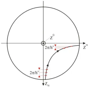
The expression (20b) implies that, when  increases from 0 to Λ(α)

1

, the observable

exp(V~_n is propagated within the domain D in the direction Z0 increasing from 0 to Λ(α)

1

. At the same time. exp(V~_nis propagated transversally towards the center of D in the directions of decreasing Z, and independently towards the periphery of D in the directions of increasing Z. That latter propagation makes of course exp(V~_{n disappear into the}

environment of D. That loss is compensated by the entrance into D of fresh exp(V~_n

coming from the environment in the direction of decreasing Z. Those propagations are represented on the figure 1.

Figure 1  Propagation of the observable exp(V~_n in a quadrant Z Zf a domain D limited by the outer

circle when  and thereby Z0 increases from 0 to Λ(α)

1

along an hyperbola Z.Z = constant. The figure shows also the increaseof the wave numbers h in Z of exp(Vn

~



A crucial point is that the propagation of exp(V~_n in the direction of decreasing Z is accompanied by the multiplication by a factor exp(()of its wave numbers h in Z as

shown on the figure 1. At the same time the propagation of exp(V~_nin the direction of increasing Z is accompanied by a division exp((() By virtue of the statement (17b) those multiplication and division apply to the observable exp(V~_n in all domains D, like

We are led at this point to choose the basic time scale  introduced in t§ II A of the order of the scale time

Λ(α) 1

. We may then state thatthe wave numbers happlicableto

exp(V~_n = exp(KVn

~

= V~_n1 are the wave numbers h applicable to V~_n multiplied by a factor exp(()

Λ(α) 1

) ~ 2. On the contrary the wave numbers h applicableto V~_n1 are

the wave numbers h applicable to Vn

~

divided by exp(() Λ(α)

1

) ~ 1/2. Of course the

wave numbers applicableto exp(V~_n= V~_n1 are the wave numbers happlicable to Vn

~

multiplied by ~ 2. and the wave numbers h’are the wave numbers h divided by ~ 2. Via an allowed iteration starting from n = 0 to n > 0, it appears that the wave numbers h displayed by V~_{n for n >0 are the wave numbers h} displayed by

V

~

₀, assumed above of the order of

Δ(α) π

 , multiplied by a number of the order of (2)n. The wave numbers h displayed by Vn

~

for n >0 tend on the contrary to decrease compared to the wave numbers h displayed by

V

0

~

, assumed also of the order of

Δ(α) π

 . However they remain of the order of the numbers h displayed by

V

~

₀, because of the action of the laws of motion of the cosmos prevailing in addition to the laws (14a,b,c) in the periphery of D. An allowed iteration starting from n = 0 towards n < 0 leads to state that the wave numbers h displayed by Vn

~

for n < 0 are the wave numbers h displayed by

V

~

₀ multiplied by (2)n|. The wave numbers h remain of the

order of

Δ(α) π

 . All those results, combined with the criterion of orthogonality (17) show that, with our choice (18) of the phenomenological spaces _P and our choice  of the order of

Λ(α) 1

, the sub-spaces ~_n satisfy as desired the structural constraint (12), so that the existence of the phenomenological determinism t P(x,p)  t’ P(x,p) for t’ > t > t* is

IV  PHYSICAL MECHANISM OF THE PHENOMENOLOGICAL DETERMINISMt P(x,p)  t’ P(x,p) FOR t’ > t > t*

The basic mechanism consists of transfers of information between the sub-spaces ~_{n of} the space _K that have been considered in §III, and of transfers between the spaces ~_n and the space _P that we must introduce now. These last transfers are already taken into account by the equation (15a), according to which the phenomenological distribution t P present at

time t within _P induces a production t p) (x, ρtK   =  t P)K of the non-phenomenological

information distribution localized in the sub-space~₀ of _K.They are complemented by the production t p) (x, ρt P  

= t K)P of phenomenological distribution t P by the the

non-phenomenological information distribution t K _{It is very important that again the subspace}

0 ~

 of _{K alone is involved. We have indeed,}

t K)•VP = t K)P•VP = t K•VP)K = t K•V0

~

  VP  P

SinceV~₀



0 ~

 is orthogonal to ~_n if n is  _{0 by virtue of the orthogonalities (12), we may} state that

“ only the component of t K in 0 ~

 contributes to t K)P “ (21)

and thereby induces a production

t p) (x, ρt P   = t K)P of the phenomenological

information t P. This important point reflects that the exponentially increasing complexity in

Z or Z of the observables Vn

~

when |n| is somewhat >1 prevents these observables to influence the evolution in time of t P.

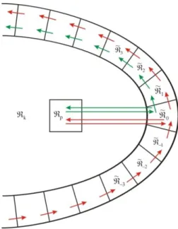
The overall dynamics is illustrated in the figure 2. The squares on that figure represent the vector spaces of observables_P and …,~_2,~_1,~₀,~₁,~₂…  _K  _P. The arrows, green if the initial condition (13) is verified, red if it is not the case, indicate 1/ the propagation in block of the non-phenomenological information t K from n

~

 to ~_nr during +, by the small arrows ; 2/ the exchanges of information between ~₀ and _P, by the long

0 n

no non-phenomenological information t K is produced after t* in that space



  0 n n ~ by the only available motion, namely the propagation in block from ~n_0 to n

~

during each interval + . The space



  0 n n ~

is accordingly after t* empty of information.

Figure 2. Schematic motion of the phenomenological and non-phenomenological information when the initial condition (13) is fulfilled (green arrows) and not fulfilled (red arrows).

However, the phenomenological information t P within P permanently produces via the

long green arrow from _P to ~₀ new components K into the space 0

~

 . A component K

produces in its turn a variation t p) (x, ρt P  

of t P into the space P via the long green arrow

from ~₀ to _P. However, after a time interval +, it enters, via the small green arrow from

0 ~  to ~₁, the space



  0 n n ~

. Because of the statement (21), once in that space it no longer influences the evolution of t p. The back and forth motion of  K from P to 0

~

 and then from ~₀ to _P during each interval + is the unique physical origin of the variation

t p) (x, ρt P  

K goes after an interval + from (0)

~

 to ~(1), then from ~(1) to ~(2), etc, via small green arrows, its wave numbers h(0), h(1), etc in Z are multiplied by O(2). The corresponding exponential increase as O(2n) of the wave numbers h(n) of the information contained in the spaces ~(n) obviously implies that they cannot be handled by the observers. That information is both inaccessible by the observers and without influence on the evolution of the phenomenological information t P(x,p). That point is in fact the key mechanism by

which the fundamental determinism t(x,p)  t’(x,p) (t’,t) generates the

phenomenological determinism t P(x,p)  t’ P(x,p) for t’>t>t*. The mere fact that the

spaces



  0 n n ~

are empty may seem surprising if not impossible. The explication is perhaps that the cosmos is quasi inexistent at the limit containing the primordial time t* between the two possibilities of existence for t > 0 and for t < 0. If that explication is correct, it explains also the fact that an observer may anticipate a phenomenological information t P(x,p) and

even organize an advantageous improvements of its environment within _Pat the condition to leave irretrievable the state of the cosmos before the considered improvement.

If the condition (13) is not realized, and the red arrows replace the green arrows, a non-phenomenological information t K is present in the space



  0 n n ~

. It moves when t increases

towards spaces ~_n with a lower n, via the small red arrows, without influencing t 

 _

t P

within _P because of the statement (21), until it reaches the space ~₀, where it does influence the derivative

t 



t P, via the long red arrow from 0

~

 to _P, by components reflecting the state of t K in the space



  0 n n ~

without correlation with t P. The autonomy of

the phenomenological evolution is then broken and the determinism t P  t’ P for t’> t > t*

is impossible. One still note the gradual decrease along the arrow of time of the quantity of the phenomenological information in t P P, at the benefit of the quantity of non

phenomenological information t KK  P. That decrease is expressed by the equation

(2), St(t P) = =  

2 1

dt d _

t P•t P), where the form St(t P) given b by the formula (10) is

at the benefit of indelible correlations which dissolve in an immense ocean of degrees of freedom [17].

The above functioning allows to soften the initial condition (13) : we may replace the

latter imposing that _n

n 



 ~ 0

is empty at the time t*, by now imposing

n n





~

is empty at the time t* for n < n*, being n* any finite positive integer, (22)

One recovers indeed at the time t*n*  the genuine condition _n

n 



 ~ 0 empty, so that a phenomenological determinism t P(x,p)  t’ P(x,p) for t’ > t > t*n* exists. In the line

of the speculation introduced at the end of § IIB, a phenomenological determinism t P(x,p)

 t’ P(x,p) for t <t <t*n* exists if at the time t* _n

n





~

is empty for n > n*.

V  CONCLUSION

We have considered in this article as a physical fact of first importance the existence in an hamiltonian cosmos of a phenomenological determinism, which allows the observers to anticipate with a substantial accuracy a specific phenomenological fraction t P(x,p of the

fundamental Boltzmann-Gibbs distribution t(x,p). Unlike the fundamental determinism

governing exactly in both time directions the fundamental distribution t(x,p), the

phenomenological determinism governs the phenomenological distribution t P(x,p)

exclusively in a preferred time direction identifiable with an arrow of time perceived by the observers. We have selected by the statement (18) a phenomenological sub-space _Pof observables such that the projection of t(x,p) into P _{plays the role of} t’ P*(x,p). This

phenomenological determinism applies if t is beyond an initial time t* where the fundamental distribution t*(x,p) realizes the simple condition (13) or (22). Apart from that poorly binding

initial condition, the phenomenological determinism t P(x,p)  t’ P(x,p) for t’>t>t*. is a

The key mechanism that ensures the existence of the phenomenological determinism is that the phenomenological distributiont P(x,p)  P may experience during a short time

interval  a forward and backward transfer of information between the phenomenological space _Pand the non- phenomenological space _K orthogonal to _{P. Those transfers play} an essential role in the evolution in time of the phenomenological distribution t P(x,p). The

existence of the phenomenological determinism comes from the fact that, just after the time , the non- phenomenological distribution t K(x,p) produced in the space K by t P(x,p)

becomes at an exponential rate complexified in (x,p) and thereby unable to influence the evolution in time of t P(x,p). That evolution at time t is thus practically determined by the

value of t P(x,p) just before the same time t. This means, under the restriction (4), that the

time scale  is much smaller than the time scale phen of the evolution of t P(x,p) around

(x,p), the autonomy of the evolution of t P(x,p) along the arrow of time and thereby the

existence of the phenomenological determinism t P(x,p)  t’ P(x,p) for t’>t>t*.

The physical importance of that phenomenological determinism comes from the fact that it is the cause of the irreversible thermodynamic behavior of the cosmos along the arrow of time perceived by the observers, and explains the various physical facts linked to that behavior. The first of these physical facts is that the observer may anticipate phenomenological information in the space _{P at the condition of leaving irretrievable the} state of the cosmos before that anticipation. In addition, the phenomenological determinism defies the phenomenological information carried by t P(x,p) as the only one accessible to

the observers. The non-phenomenological information t K(x,p) that t P(x,p) permanently

produces in the space _K accumulates undamped in the latter along the arrow of time with an exponentially increasing complexity in (x,p). The quantity of accessible information contained in t P (x,p) thus appears as the negentropy present at each time in the cosmos,

ineluctably decreasing along the arrow of time at the benefit of the quantity of inaccessible information contained in t K(x,p). The decrease of that negentropy gives a natural basis to

generalized H theorems.

determinisms in magnetically confined plasmas. One of us (A.S.) warmly thanks Dr Marc Dubois for very useful discussions.

REFERENCES 

[1] M. C. Mackey in « Time’s arrow : The Origins of Thermodynamic Behaviour”, chapter 2, Springer Verlag, 1992.

[2] C. K. Zachos, D. B. Fairlie, T. L. Curtright in “Quantum Mechanocs in Phase Space”, chapter 1 and 2, World Scientific Publishing, New Jersey, 2005.

[3] L. D. Landau and E. M. Lifshitz, in “Statistical Physics”, chapter 1, Pergamon Press, 1958.

[4] R. Balian, in “From Microphysics to Macrophysics”, chapters 2 and 4, Springer Verlag, 2007.

[5] C. Cercignani, in “The Boltzmann Equation and its Applications”, chapter 2, Springer Verlag, 1988.

[6] L. D. Landau, Soviet Physics JETP, 16, 574, 1946.

[7] R. Jancel in « Foundations of Classical and Quantum Statistical Mechanics », chapter 5, Pergamon Press, 1969.

[8] R. Zwanzig, Journal of Chemical Physics 33, 5, 1960 [9]Samain and Garbet, 2020, submitted to Physica A

[10] A. Samain and F. Nguyen, Plasma Phys. and Control. Fusion 39, 1997.

[11] P. C. W. Davies, in “Physical Origins of Time Asymmetry”, edited by J. J. Halliwell, J. Perez-Mercader, W. H. Zurek, chapter 7, Cambridge University Press, 1994.

[12] J. J. Halliwell in “Physical Origins of Time Asymmetry”, edited by J. J. Halliwell, J. Perez- Mercader, W. H. Zurek, chapter 25, Cambridge University Press, Cambridge, 1994.

[13] J. L. Lebowitz, Physica A, 263, 1999.

[14] M. Kruskal, Journal of Mathematical Physics, 3, 806, 1962.

[15] A. J. Lichtenberg and M. A. Lieberman, in “Regular and Stochastic Motion”, chapter 3 and 5, Springer Verlag, 1983.

[16] RV. I. Oseledec, Trans. Moscow Math. Soc. 19, 197, 1968.

[17] I. Prigogine et I. Stengers in « Entre le temps et l’éternité », chapter 1 and 5, Flammarion, Paris, 1992.