HAL Id: inria-00384542
https://hal.inria.fr/inria-00384542
Submitted on 15 May 2009
HAL is a multi-disciplinary open access
archive for the deposit and dissemination of
sci-entific research documents, whether they are
pub-lished or not. The documents may come from
teaching and research institutions in France or
L’archive ouverte pluridisciplinaire HAL, est
destinée au dépôt et à la diffusion de documents
scientifiques de niveau recherche, publiés ou non,
émanant des établissements d’enseignement et de
recherche français ou étrangers, des laboratoires
Tahiry Razafindralambo, David Simplot-Ryl
To cite this version:
Tahiry Razafindralambo, David Simplot-Ryl. Mobile Sensor Deployment with Connectivity
Guaran-tee. [Research Report] RR-6936, INRIA. 2009. �inria-00384542�
a p p o r t
d e r e c h e r c h e
N 0 2 4 9 -6 3 9 9 IS R N IN R IA /R R --6 9 3 6 --F R + E N G Thème COMMobile Sensor Deployment with Connectivity
Guarantee
Tahiry Razafindralambo — David Simplot-Ryl
N° 6936
Centre de recherche INRIA Futurs Parc Orsay Université, ZAC des Vignes, 4, rue Jacques Monod, 91893 Orsay Cedex (France)
Guarantee
Tahiry Razafindralambo
∗, David Simplot-Ryl
†Th`eme COM — Syst`emes communicants ´
Equipes-Projets POPS
Rapport de recherche n° 6936 — Septembre 1997 — 28 pages
Abstract: In this paper, we consider the self-deployment of wireless sensor network. We present a deployment strategy for mobile wireless sensor network which maximizes the sensors covered area with the constraint that the resulting deployment provides a connected topology. Our deployment algorithm is dis-tributed and is based on subset of neighbour for motion decision. Each node is considered as a particle and its movements are governed by the interaction with a part of its neighboring nodes. The interacting neighbors and the node’s direction are chosen based on the local relative neighborhood graph. Analytical and simulations results show that the resulting graph is connected, the distance between two sensors is maximized and thus the area covered is maximized. We also show by extensive simulation that some simple modifications of our algo-rithm allow different coverage schemes such as Point of Interest coverage and barrier coverage.
Key-words: mobile sensor network, deployment
de connexit´
e
R´esum´e : Dans cet article, nous consid´erons le d´eploiement autonome d’un r´eseau de capteurs. Nous pr´esentons une strat´egie de d´eploiement pour des cap-teurs mobiles qui maximise la surface couverte par chaque capteur avec comme contrainte que le r´eseau r´esultant soit connect´e. Notre algorithme est distribu´e et le mouvement et la direction de chaque capteur se calcule en fonction d’un sous ensemble du voisinnage de ce capteur. Le sous ensemble de voisins que nous utilisons fait partie du sous graphe RNG. Une analyse et des simulations mon-trent que le graphe r´esultant est connect´e, que la distance entre deux capteurs est maximis´ee et de ce fait, la surface couverte est aussi maximis´ee.
1
Introduction
Maximizing coverage of a monitored area in wireless sensor networks has re-ceived a lot of attentions these past years. Optimizing sensor placement is a difficult problem even for deterministic and static deployment. Although these deterministic deployment can provide optimal solution, they are not always fea-sible since they require precise knowledge of the monitored area. Controlled deployment, or online deployment are only feasible when accurate position of sensor is available and when nodes have motion capabilities. However, the main advantage of online deployment is the possibility to obtain particular topologies which can reduce energy consumption, optimize routing scheme or flooding, etc [4]. Moreover, different coverage schemes such as barrier coverage [12] or sweep coverage [6] can be obtained with online deployment.
During the online deployment, the evolving graph may have different prop-erties. Controlling the dynamic graph of mobile sensors networks is a fun-damental issue in sensor deployment. The most important properties of the dynamic graph are connectivity, edge length, and node degree. Indeed, in the area of mobile communication and especially while considering wireless sensor networks the main challenge is to maintain connectivity from any sensors to the sink. This connectivity allows an external entity to update the behaviour of all the sensors and to gather information from the sensors by using multi-hop communication. Moreover, authors of [20] have shown that there exists an opti-mal communication range that minimizes energy consumption in wireless sensor networks. The node degree is also an important characteristics since reducing this degree may reduce communication overhead and increase the performance of communication protocols.
In this paper we consider the problem of deploying and controlling a fleet of mobile sensors which maximizes the area covered by all the sensors while keeping the graph of mobile sensor connected at each step of the deployment. Our first assumption is that the sensors are all within communication range of each other. This first configuration, strongly reduce the total covered area. From this initial configuration, we use a simple repelling force to expand the network. Unlike previous work especially on virtual potential field, we only use the repelling force from a subset of neighborhing nodes. This subset is chosen based on the neighbors in the Relative Neighborhood Graph (RNG) [22] of the node. In order to avoid disconnection, the node has to maintain its connections to its RNG neighbors. After the first repelling process, some connections between the node and its previous neighbors are lost which increases the area covered. Analytical and simulation results show that our proposed deployment algorithm maintains graph connectivity at each step, that the average edge length is close to the desired one, that the average node degree is ∼ 4 and that the coverage provided by our algorithm is close to a regular square coverage pattern.
Our deployment algorithm is fully distributed, asynchronous and simple enough to take into account obstacles, or specific fields constraints. Moreover, since the directions and the movements of a given node is only constrained by the connections to its RNG neighbors, the node’s direction can be govern by any requirements which allows our algorithm to be adapted to different coverage schemes.
• We provided a deployment algorithm for mobile sensor networks.
• Our algorithm maintain connectivity at each step of the deployment, pro-vided that the initial network is connected. We use the Relative Neigh-borhood Graph to preserve connectivity and prove that the network is connected at each step of the deployment.
• We divide our algorithm into 2 major parts. The connectivity
preserva-tion part and the deployment part. This distincpreserva-tion allows us to provide
different deployment schemes while keeping connectivity. In this paper, results on area coverage maximization, Point of Interests (POI) coverage and barrier coverage are provided.
• For the area coverage maximization algorithm, we show that the resulting coverage is close to a regular square pattern coverage. We also prove that the nodes do not oscillate, that the network is expanding and that the algorithm will eventually terminate.
• For the POI coverage, we show by simulation that the nodes used for connect the POI and a base station is independent from the number of node in the network.
• For the barrier coverage, we show by simulation that the node form a line between their starting point and their end point. We also show that multiple barriers are possible.
The rest of this paper is organized as follow. In Section 2 we give a state of the art on area coverage with a focus on mobile sensor coverage. In section 3 we give an overview of assumptions and notations used in this paper. Section 4 details our deployment algorithm and Section 5 provides an analysis of this algorithm and simulation results are given in Section 6. In Section 7, we give some simulation results on Point of Interest coverage and barrier coverage. The conclusion and some possible future works are provided in Section 8.
2
Related Work
Maximal coverage for monitored area is the goal of wireless sensor networks that has received most attentions in the past years. There are mainly three categories of works that focus on coverage optimization in the literature. 1) Random de-ployment of sensors. In this category, a huge number of sensors are deployed randomly and later, activity scheduling algorithms or power control technique are used to reduce the network density [3, 18]. Algorithms in this category mainly focus on maximum area coverage with minimum active sensors and con-nectivity constraint. 2) Alternatively, off-line computation of sensor placements can be done [11, 16, 1]. In this category, network performance, connectivity and area coverage are considered for node placement. The works presented in these papers give a overview of possible off-line node placement and their coverage performances with connectivity constraints. 3) Sensor repositioning scheme. As the work presented in this paper mainly focus on the sensor (re)positioning or online placements, the rest of this section is devoted to this category of the cov-erage issue. For the interested reader a complete state of the art can be found in [23].
The local dispersion of multiple mobile sensors (or mobile robots which em-bed sensors) was first developed in [2] to achieve a better coverage of the whole sensing field. In [2] Batalin and Sukhatme argue that the local dispersion is the basis of increasing global coverage. In this approach, sensors are mutually repelled by each other within their communication range. Their approach is inspired by the diffusive motion of fluid particles.
The artificial potential field concept was first proposed by Khatib in [10]. Potential field theory was used to compute path planning algorithms for mobile robots in [17, 19]. Algorithms for coverage maximization used with potential field theory were developed in [7] and [15]. These algorithms build local virtual force between neighboring nodes to compute their desired motion or placement. In [15], the deployment strategy is constraint by the fact that each node must have at least K neighbors. A repelling force is computed to increase the coverage of the network while an attracting force tries to maintain the node degree. In [24] the authors focus on network connectivity and do not properly consider area coverage. They translate the connectivity conditions to differentiable constraint on individual node motions.
In [21], the authors also use potentiel field concept for deploying mobile robots. The proposed deployment tries to preserve the graph connectivity by checking at any time if the graph is connected. In the proposed deployment, a message is regularly flooded in the network. It is important to notice here taht this regular flooding is resource consumming in wireless sensor network. If a mobile sensor does not receive this message it assumes that it is disconnected and move toward its last position or some predefined intermediate destinations. The closest work to ours is proposed in [14]. The authors use local geometry combined with potential field theory to maximize the area coverage of mobile robots. They use a Neighbor-Every-Theta (NET) graph to compute the nodes movements. The authors apply the same forces as described in [15]. By using a combination of mutually opposing forces, each node maximizes its coverage while maintaining the NET condition of having at least one neighbor in every θ sector. In the proposed deployment, when the number of neighbors is close to the number required to satisfy the NET condition, a priority is used to maintain the neighbors which contributes to larger sector. An attracting force is applied to those neighbors to maintain connectivity. Moreover, the deployment algorithm described in [14] needs priority exchanges between neighboring nodes to ensure forces symmetry which increases the message overhead of the algorithm and makes it degrades when messages are lost. It is worth noting that in [14] for a specific θ ≤ 2π3 the graph can embed an RNG graph. However, the distributed algorithm deployment proposed by the authors cannot guarantee connectivity.
In our work, we use the property of the Relative Neighborhood Graph to maintain connectivity and increase the area coverage. Most of the proposed solutions in the literature (except [24]) do not guarantee network connectivity. To the best of our knowledge, our work is the first that maximizes the covered area while preserving connectivity.
3
Basic idea of our approach
In this section, we present the notatations and assumptions used in the rest of this paper. We also outline the basic idea of our approach an motivate the choice of the RNG graph.
3.1
Notations and assumptions
Definition 1 Let G(V, E) be the graph representing the sensor network. V is the set of vertices each one representing a sensor. E ⊆ V2 is the set of edges; E = {(u, v) ∈ V2 | u 6= v ∧ d(u, v) ≤ R}, where d(.) is the euclidean distance
between node u and v and R is the communication range. G(V, E) is our model of the sensor network.
Definition 2 N (u) = {v ∈ E | d(u, v) ≤ R}. N (u) is the set of 1-hop neighbors
of node u.
Definition 3 Let RN G(G) be the relative neighborhood graph extracted from
G(V, E). RN G(G) = (V, Erng), where Erng = {(u, v) ∈ E | ∄w ∈ (N (u) ∩ N (v)) ∧ d(u, w) < d(u, v) ∧ d(v, w) < d(u, v)}.
Assumption 1 We assume that each sensor has its exact position denoted by
(x(u), y(u)) for node u. This position can be provided by any internal
mecha-nisms or external entities such as GPS.
Definition 4 RN G(u) is the set of node u neighbors which are part of the RN G(G) graph RN G(u) = {v|v ∈ N (u) ∩ RN G(G)}. We denote by |RN G(u)|
is the number of node in RN G(u).
Definition 5 RN G+(u) (resp. RN G−(u)) is the furthest node that is part of RN G(u), the distance between u and RN G+(u) (resp. RN G−(u)) is denoted
by d+(u) (resp. d−(u)).
Definition 6 ν is the speed of a given node. ν is chosen from a given interval [0, νmax].
Assumption 2 Each node gathers its neighborhood state periodically and com-pute its next position based on its neighborhood every δ. We also assume that each node regularly sends a HELLO message containing its ID and position with a frequency higher than δ/2 for computation accuracy.
3.2
Basic idea
Our deployment algorithm is distributed and is based on potential field theory. Each node is considered as a particle and its movements are governed by the interaction with a part of its neighboring nodes. The interacting neighbors and the node’s direction are chosen based on the relative neighborhood graph. The RNG graph [22] is a good solution since its computation only requires local information. Moreover, the use of the euclidean distance for computing the RNG graph can strongly reduce the mean degree of the graph. Compared to a unit disk graph, the mean density of an RNG graph is ∼ 3 [22]. While removing
some edges from the initial graph, the graph RN G(V, Erng) ⊆ G(V, E) also preserves the connectivity, provided that the initial graph G(V, E) is connected. The properties provided by the RNG graph are very useful for preserving connectivity. In our algorithm, any graph that reduces the neighborhood while keeping connectivity can be used to compute the repelling force such as Gabriel Graph (GG) of Spanning Trees. We can also try to increase the connectivity by using graph such as k-RNG graphs, k-GG, etc., [8].
Moreover, we have divided our algorithm into two distinct parts. The di-rection computation schemeand the connectivity preservation scheme. This distinction allows us to provide different deployment schemes while preserv-ing connectivity. Therefore with some simple modifications on the deployment scheme we can fit different requirements of mobile sensor deployment applica-tions.
4
Protocol description
The protocol is divided into 4 parts described in Algorithm 1. Part I, III, and IV are used for connectivity preservation and Part II is used for the direction computation scheme. In the first part, based on the information gathered from its neighborhood, a node u computes its movement speed. This speed is the maximum possible speed to allow fast deployment of nodes. We divide this speed by two to take into account the worst case movement of RN G+(u). We also avoid null speed to allow some small movements for node u. This allow nodes that are at distance R to move toward each other. After part I, the nodes knows its deplacement speed ν. In the second part, node u computes its direction. The direction chosen by node u depends on its neighborhood. Node u goes farther from all RN G(u) nodes except those at distance R by using the resulting vector−→∆. Moreover, we use a weighted sum to compute the resulting vector and increase the impact of closer nodes in the direction of node u (Line 2 of Part II). In Line 3 of Part II we only compute the normalized direction. If the direction is −→0 and two nodes are at the same place, or if the node is disconnected (Line 6 of Part II), a random or predefined direction is choosen. After part II, a normalized vector−→∆ gives the direction of node u. In the third part, node u computes the distance of its deplacement. This distance is choosen in a given range (Line 2 of Part III). The upper bound of this range is computed based on d+(u) and R (Line 1 of Part III). It is limited by the communication range (R − d+(u)) which forbids a node u to be disconnected from its RN G(u) nodes. We also allow nodes to make small movement if the upper bound is 0. In Line 2 of Part III, we compute a speed called νoth which is the maximum speed of the other nodes in RN G(u). Based on the range and the speed of other nodes, node u computes the maximum possible distance given that in its new position1 it remains connected to its RN G(u) nodes while assuming that the RN G(u) nodes have taken the worst direction decison (Line 3 of Part III). At the end of Part III, node u knows its maximum deplacement dopt. Because computing such an optimum distance can be resources consumming for a sensor with limited capacity in the implemented version we incrementally try a limited number of possibility to approximate dopt. In the last part, node u moves to its
1
Algorithm 1MSD (Mobile Sensor Deployment) protocol PartI — Speed computation on nodeu:
1: ν=R−d+(u)δ×2 ;
2: ν= min (max(ν, ǫ), νmax);
PartII — Direction computation on nodeu:
1: −→∆(x(∆), y(∆)) is the direction vector of u
2: −→∆ = X v∈RN G(u) d(u,v)<R (R − d(u, v)) × ||−vu||→ 3: −→∆ = − → ∆ ||−→∆||; 4: if((→−∆ ==−→0 && d−
(u) == 0) || (|RN G(u)| == 0)) then
5: Choose a random/predefined direction;
6: end if
PartIII — Distance computation for nodeu:
1: dmax= max (ǫ, R − d+(u));
2: νoth=R−d+(u)δ×2
3: dopt= {d ∈ [0, dmax] | ∀v ∈ RN G(u), d(unew, v) + νoth× δ < R}
4: where unew is the new position of node u based on:
5: -speed ν from Part I.
6: -direction−→∆ from Part II.
7: -distance d.
PartIV — Nodeu destination and movement:
1: move to unew using :
2: -speed ν from Part I.
3: -direction−→∆ from Part II.
4: -distance doptfrom Part III.
5: -Take field border into account
next position based on dopt, − →
∆ and ν, by taking into account constraints from the field border. We distinguish Part III and Part IV since for the latter one we can use results from robotics to compute node’s motion such as in [13] in which an obstacle avoidance algorithm for path planning is described.
It is important to notice here that Part II of Algorithm 1 is completely independent from the other parts. This is an important properties since we can easily modify the direction of the node to fit some other requirements such as moving towards some points of interest.
5
Algorithm properties
In this section we demonstrate that at each step of our algorithm, the graph is connected, that the graph is expanding and that there is no oscillation. We con-sider that each link is symmetric and sensors are equipped with omni-directional antenna. We also assume that the transmission power of each node is fixed and thus that the graph can be modelled as a UDG (unit disk graph.
In the sequel, node are running the same algorithm (Algorithm 1) with the same parameters. We assume a discretized time indexed by i ∈ N. At t = 0, all nodes are connected. Nodes are uniquely identified and are called ni, i ∈ [0, ..., N − 1] where N is the number of nodes. Note that in the sequel, node’s position are identified by nji where i is the node id and j the time index. We use n0 and nj0 to identify the nodes and their positions.
5.1
Connectivity
Lemma 1 If at time t = T the graph is connected. If all node are synchronized and run algorithm 1 in a sequential way that is in a given interval [t, t + 1[ only one node run the algorithm and reach is new position during this interval; then
∀i > T the resulting graph at time t = i is connected.
Proof. The proof of this theorem depends only on the distance covered by the node. This distance is computed in Part III of Algorithm 1. We know that at t = 0, the network is connected (initial condition). At t = 0, n0
0 run algorithm 1. The maximum distance covered by n0
0is dopt= {d ∈ [0, dmax] | ∀v ∈ RN G(n0
0), d(n10, v) + νoth× δ < R}. At time t = 1 the new position of n00 is n1
0. The condition on dopt, avoids n0 to be disconnected from its RN G(n00) neighbors. Indeed, at time t = 1 ∀u ∈ RN G(n0
0), d(n10, v) < R (note that ν × δ > 0 and νoth× δ ≥ 0) since the nodes run algorithm in a sequential way, during the time [t, t + 1[ no other node is moving. Thus n1
0 is still connected to its RN G(n0
0). Based on the properties of the RNG graph, the graph at time t = 1 is therefore still connected. We know that if the graph is connected at t = 0, it is also connected at t = 1. We can state that if at any t = i, i > 0 the graph is connected, at t = i + 1 the graph is still connected and we can also state that if at a given time t = T the graph is connected at any time t > T the graph is still connected.
Theorem 2 If at time t = T the graph is connected, ∀t = i, i > T the resulting graph at time t = i is connected.
Proof. The Lemma 1 shows that in a synchronized environment if the initial graph is connected the graph remains connected. In an asynchronous environ-ment, nodes can run algorithm 1 at any time. Let nT
i and nTj be two nodes and nT
i and nTj are connected a time t = T . Let nTi ∈ RN G(nTj), nTj ∈ RN G(nTi) and d(nT
i, nTj) = d+(nTi ).
CASE 1: Let us assume that the two nodes run Algorithm1 at the same time, and that the two nodes are moving to the opposite direction of each other. The maximum distance covered by node nT
j depends on its speed and the sampling time δ. Since d(nT
i, nTj) ≤ d+(nTj) the maximum speed of node nTj computed in Line 1, Part I of Algorithm 1 is νj =
R−d+(nT j) δ×2 ≤ R−d+(nT i) δ×2 = νi (the speed of node nT
i). Therefore, the maximum distance covered by node nTj during δ is at most νi× δ. Notice that the position of node nTi is nT+δi after its movement. The computation of doptfor node nTi in Line 3, Part III of Algorithm 1 includes the worst case movement of the nT
j which still maintains connection to all its RN G(nT
i) nodes after its movement. CASE 2: Let us now assume that d(nT
i , nTj) = R = d+(nTi). In that case, νi = νj = ǫ and νoth = 0 for both nodes. If both nodes are moving to the opposite direction, condition in Line 3, Part II of Algorithm 1 is not satisfied for a value of d > 0. If one of the nodes, let say ni, is moving toward the other node and (nj) moves to the opposite direction of ni, dopt= 0 for node nj, for the same reason, and dopt≥ 0 for node ni since condition in Line 3, Part II of Algorithm 1 can de verified.
If the connection to the farthest RNG neighbor is maintained, the connection to close RNG neighbors is also maintained. For that, let us assume node nT
RN G(nT
i ) with d(nTi , nTk) ≤ d(niT, nTj), the speed of node nTk is at most νk = R−d+(nT
k)
δ×2 ≤
R−d(nT
i,nTk)
δ×2 . Therefore, the maximum distance covered by node nT
k is at most νk × δ. The worst case movement for the two nodes nTi and nT k leads to a distance d(n T+δ i , n T+δ k ) = d(nTi, nTk) + νk × δ + νi× δ ≤ R by replacing νk and νi by their value (or upper bounds) and since d(nTi , nTk) ≤ d(nT
i , nTj). Therefore, the movement of node nTi does not disconnect it from its RNG neighbors. Network connectivity is thus kept.
5.2
Oscillations
0
(0,0)
1
(6,0)
2
(14,0)
d
01d
12Figure 1: Example of configuration where node 1 oscillates between positions (6, 0) and (8, 0). In this case, node 0 and 2 are static, R = 12 and node 1 runs Algorithm 1.
While running Algorithm 1, nodes can oscillate. Indeed, the direction com-putation in Part II of Algorithm 1 cannot avoid a node u from choosing a direction−−−→∆i+δand a distance di+δ
opt at time t = i + δ if at time t = i its direction was−∆→i = −−−−→∆i+δ and its distance di
opt= d i+δ
opt. A simple numerical example of this oscillation is given in Figure 1. In this case we assume that node 0 and node 2 are fixed and R = 12, at time t = i nodes are in the configuration pre-sented in Figure 1. Node 1 direction’s at time t = i is −∆→i = (1, 0), νi = 8
2×δ, dmax = 4. Based on Line 3 of part III in Algorithm 1, diopt= 2, since it is the maximum value that can verify the condition. Indeed, for di
opt = 2, we have d(1, 0) + di
opt+ νoth× δ = R with νoth× δ = 4, d(1, 0) = 6 and diopt= 2. Here node 1 does not know that node 0 is fixed. Next position of node u is thus u(8, 0). Node 1 will thus oscillate from position (6, 0) and (8, 0) since the same computation applies when node 1 is at position (8, 0).
To avoid this oscillation, it is important to have di+δopt < diopt. This condition can be easily added in our algorithm, by adding a condition on dopt. We can modify Line 2 of Part II in Algorithm 1 by the following:
[2-0]−→∆ = 1 p X v∈RN G(u) d(u,v)<R (R − d(u, v)) × ||−vu||→ [2-1] E(x(u) + x(∆), y(u) + y(∆));
p ∈ R is a constant and p ≥ 2. The point E gives the movement end point of node u. In order to take this end point into account, we add the following condition after Line 3 of Part III in Algorithm 1:
[3-0] dopt= {d ∈ [0, dmax] | ∀v ∈ RN G(u), d(unew, v) + νoth× δ < R};
[3-1] if (dopt> d(u, E) )
[3-2] dopt= d(u, E);
Definition 7 Let P OS(ui) ⊆ RN G(ui) (resp. N EG(ui) ∈ RN G(ui)) be the
set that provides direction −∆→i (resp. −−∆→i) for node u at time t = i. P OS(u)
and N EG(u) can be replaced by their respective gravity center f and b. Figure 2 shows a graphic representation of P OS(u) and N EG(u).
f
u
b
P OS(u)
N EG(u)
Figure 2: Represention of P OS(u) and N EG(u) sets.
Lemma 3 For p ≥ 2, if we assume that RN G(u) does not change between t = i and t = i + δ and that two nodes cannot have the same location, if at time t = i a node u chooses a direction−∆→i 6=−→0 and a distance di
opt> 0, at time t = i + δ,
if node u chooses a direction ||−−−→∆i+δ|| = −||−∆→i|| then di+δ
opt < dioptfor d i+δ opt > 0. Proof. Nodes in P OS(ui) and in N EG(ui) can be replace by their gravity center f and b. Since RNG(u) is fixed between [t; t+δ], f and b do not change. If node u follows the direction−f u this means that d(u→ i, f ) < d(ui, b) at time t = i. If we assume that at time t = i + δ, ||−−−→∆i+δ|| = −||−∆→i|| we have d(ui+δ, f ) > d(ui+δ, b). We know that
d(ui+δ, f ) = d(ui, f ) + di opt d(ui+δ, b) = d(ui, b) − di
opt Based on our new algorithm,
di+δopt ≤ 1
p[(R − d(u
i+δ, b)) − (R − d(ui+δ, f ))] di+δopt ≤
1 p[d(u
i+δ, f ) − d(ui+δ, b)] di+δopt ≤
1 p[(d(u
i, f ) + di
opt) − (d(ui, b) − diopt)] di+δopt ≤
1 p[2.d
i
opt− (d(ui, f ) − d(ui, b))] 2
pd i
opt ≥ di+δopt + 1 p[d(u i, b) − d(ui, f )] 2.di opt− p.d i+δ
opt ≥ d(ui, b) − d(ui, f ) Therefore, for p ≥ 2, di
opt− d i+δ
Lemma 4 For p ≥ 2, if we assume that two nodes cannot have the same lo-cation, if at time t = i a node u chooses a direction −∆→i 6= −→0 and a distance di
opt> 0, at time t = i + δ, if node u chooses a direction || −−−→
∆i+δ|| = −||−∆→i|| then di+δopt < diopt for di+δopt > 0.
Proof. In Lemma 3 we showed that when the RN G(u) is fixed, there is no oscillation. There are four cases that may happen:
• d(ui+δ, fi+δ) > d(ui, fi) and d(ui+δ, bi+δ) < d(ui, bi). This is the case de-scribed in Lemma 3 where d(ui+δ, fi+δ) ≥ d(ui, fi)+di
optand d(ui+δ, bi+δ) ≤ d(ui, bi) − di
opt
• d(ui+δ, fi+δ) < d(ui, fi) and d(ui+δ, bi+δ) < d(ui, bi). Since d(ui+δ, uf+δ) < d(ui, uf), the resulting effect of−−−−−−→fδ+iuδ+i is greater than−−→fiui. Therefore di+δopt < di
opt.
• d(ui+δ, fi+δ) > d(ui, fi) and d(ui+δ, bi+δ) > d(ui, bi). In this case, the resulting effect of−−−−−→bδ+iuδ+i is lower than−−→biui. Therefore, di+δ
opt < diopt. • d(ui+δ, fi+δ) < d(ui, fi) and d(ui+δ, bi+δ) > d(ui, bi). In this case ||−−−→∆i+δ|| =
||−∆→i|| which is inconsistent with our hypothesis and shows that node u fol-lows the same direction.
Lemma 3 and 4 show that there is no oscillation between two points. Yet, it is difficult to prove that there is no oscillation between more than two points, some simulation results strongly suggest that our algorithm does not oscillate.
5.3
Expansion
Theorem 5 Let G(V, Ei), be connected at time t = i. Let m
1 and m2 ∈ V
and d(mi
1, mi2) = max
u,v∈V2{d(u, v)} at time t = i. Then at t = i + δ, d(m
i
1, mi2) ≤ d(mi+δ1 , mi+δ2 ).
Proof. Let us assume that d(mi
1, mi2) > d(mi+δ1 , mi+δ2 ). The direction of mi 1 is thus −−→ ∆i m1. −−−→ mi
1mi2 > 0. There exists at least one node u which provides this direction−−→∆i
m1 on node m
i
1. This means that d(mi1, u) > d(mi1, mi2) which is inconsistent with our assumption that d(mi
1, mi2) = max
u,v∈V2{d(u, v)}. Since
G(V, Ei) is connected, algorithm will not enter condition in Line 4, Part II of algorithm 1.
This Theorem shows that the diameter of the network is expanding which means that the surface coverage is also always increasing.
5.4
Termination
Our algorithm will eventually terminate. That is to say, a given node u will eventually stop moving. In Algorithm 1 a node u stops moving only under two conditions:
1. −→∆ =−→0 . This condition is in Line 4 of Part II. If this condition is verified, that means that node u has reach its ‘destination’. Here the ‘destination’ is a general term which means that the resulting repelling vector from RN G(u) nodes is −→0 . A simple example of this condition is given in Figure 3(a). In this figure, the value of −→∆ computed by node 1 is −→0 . Here, if node 2 or node 0 moves, in its next movement node 0 will probably move.
2. dopt = 0. This condition is valid when one of the node in RN G(u) is at distance R and the direction computed by u goes farther from this particular node. Figure 3(b) gives a simple example of this condition. Node 0 is at distance R of node 1 and 0 and 1 are repelling. Since condition in Line 3 of Part III of Algorithm 1 has to be verified, the only possible value of doptis 0. In this case,both nodes 0 and 1 are stable.
0 1 2 d d (a) 0 1 R −→∆ (b)
Figure 3: Stability of Algorithm1
Theorem 6 In a 1-dimensional field, if we assume that nodes are not co-located, the algorithm terminates.
Proof. This property comes directly from the non-oscillation properties of our algorithm proved in Lemma 3, Theorem 4 and the expansion property in Theorem 5. We can only prove this property on a 1-dimensional field, based on the proof of these Lemmas.
6
Simulation results
We evaluate the performances of our algorithm through simulations using WS-Net2. The main performance metric we use is coverage. We use a discrete way to evalute the coverage. Area is divided into a grid and we compute the number of points that are covered over the total number of point in the grid. In most of the simulations, nodes are starting from the same location in the middle of the area, we use an obstacless 2-d field. The simulation parameters are summarized in Table 1.
2
Field size 100m × 100m Sensing range 10m Max Communication range 10m Desired Communication range 10m
νmax 20ms−1
δ 5s
ǫ 0.1
Simulation time 5000s
Table 1: Summary of the simulation parameters.
6.1
Example of networks
The first results show the evolution of node’s position depending on time. We can see from Figure 4 that, as proved by Theorem 2, the graph is connected, that is it expanding (Theorem 5) and that the algorithm reaches a stability point (Theorem 6) since there is no huge difference between the graph at 1500s and 2500s.
(a) 20s (b) 100s (c) 200s (d) 500
(e) 1000s (f) 1500s (g) 2000s (h) 2500s
Figure 4: Evolution of node’s position and associated graph depending on time. In this simulation there is 40 nodes with a range of 10 on a square of 100 × 100.
6.2
Coverage
In this section, we present coverage results of our protocol. In the following simulation, we set the sensing range equal to the communication range. The area is a square of 100 × 100 and the communication range is set to 10.
We can see from Figure 5(a) that the resulting coverage of our protocol is roughly equal to a coverage provided by a square pattern. This figures show that the results is roughly the same until 90 nodes since the area cannot be fully covered. When the number of nodes is enough to cover all the area, our algorithm, because of its dynamic behaviour suffers from border effects which may prematurely stop node’s movements.
0 50 100 150 0 0.2 0.4 0.6 0.8 1 #nodes % co ve ra ge Our algorithm triangle square hexagon
(a) Coverage vs. Nodes
0 500 1,000 1,500 2,000 2,500 0 0.2 0.4 0.6 0.8 1 time % co ve ra ge 10 nodes 60 nodes 120 nodes 160 nodes (b) Coverage vs. Time
Figure 5: Coverage results. In Fig. 5(a) we compare our algorithm to off-line deployment following different regular patterns (triangle, square and hexagon). In Fig. 5(b) we plot the coverage evolution vs. Time for different node numbers.
In Figure 5(b) we can see the coverage results depending on time. This result confirms our assumption about the expansion property of our algorithm, discussed in Section 5.3. We can see that the curves are increasing.
6.3
Covered distance
In the following sections, in order to remove the border effects due to area constraints we run simulations where the number of sensors is not enough to cover the whole area. In this section, we present the distance covered by a node and show the termination of our algorithm. It is important to notice here that Theorem 6 is only valid in a 1-dimensional space. Indeed, in a 2-dimensional field there may not exit a stability condition as described in Figure 3.
20 40 60 80 20 40 60 80 100 120 #nodes d is ta n ce
(a) Distance vs. Nodes
0 500 1,000 1,500 2,000 2,500 0 20 40 60 80 time d is ta n ce 10 nodes 30 nodes 60 nodes 80 nodes (b) Distance vs. Time
Figure 6: Distance results. In Fig. 6(a) we plot the mean distance covered depending on the number of nodes. In Fig. 6(b) we plot the distance evolution for a specific node vs. Time and for different node number.
Figure 6(a) shows the mean distance covered by the nodes for different total number of nodes. We can see in this figure that the covered distance is increasing
since our algorithm makes the node expanding. We can also notice that the mean covered distance for 80 nodes is greater that the width of the field. This is due to the motion of nodes which do not go to the their final destination in a straight line.
In Figure 6(b) we plot the cumulative distance of a specific node depeding on time. This figure only shows that for these simulation parameters the observed node eventually terminates its motion since the curves become constant.
6.4
Graph properties
In this section, we comment the graph properties of our algorithm. We consider the node degree and the edge’s length. We also present some changes in of our algorithm to meet different edge lengths.
6.4.1 Degree 20 40 60 80 2 4 6 #nodes d eg re e Average min max
(a) Degree vs. Nodes
0 50 100 150 200 250 0 20 40 60 80 time d eg re e 10 nodes 30 nodes 60 nodes 80 nodes (b) Degree vs. Time
Figure 7: Degree results. In Fig. 7(a) we plot the average degree depending on the number of nodes. In Fig. 7(b) we plot the degree evolution for a specific node vs. Time and for different node number.
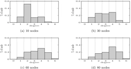
In Figure 7(a), we plot the average node degree with its confidence interval and the minimum and maximum node degree observed in the graph. This figure shows that the average degree is around 3.8 for 80 nodes. The node degree distribution is plotted in Figure 8. This figure shows that when the number of node is high, most of the nodes have a degree of 4 which confirms the coverage results where we argue that the coverage provided by our protocol is close to the coverage provided by a regular square pattern.
In Figure 7(b) we plot the degree evolution of specific node depending on time.This figure shows that node degree may increase or decrease during the simulation. We only plot the evolution until 250s since the degree does not evolve after this time. We can see that the final degree of a node is reached very early in the simulation.
6.4.2 Edge length
In Figure 9 we plot the average of the difference between R and the edge length l and normalize this value: R−l
0 1 2 3 4 5 6 0 0.2 0.4 0.6 degree % of no de (a) 10 nodes 0 1 2 3 4 5 6 0 0.2 0.4 0.6 degree % of no de (b) 30 nodes 0 1 2 3 4 5 6 0 0.2 0.4 0.6 degree % of no de (c) 60 nodes 0 1 2 3 4 5 6 0 0.2 0.4 0.6 degree % of no de (d) 80 nodes
Figure 8: Degree distribution for different number of nodes.
20 40 60 80 1 1.2 1.4 1.6 1.8 ·10−2 #nodes R − l R
Figure 9: Edge length results. We plot the difference between the length l and the communication range R, and normalize this value. That is R−l
R and l is less than 2‰. We can also see in this figure that the average edge length is independent from the number of nodes.
In the Algorithm described in 1 we mainly focus on expanding the network to maximize the covered area. It may be interesting to add a constraint on edge length. This can be easily done by replacing the Line 2, Part II of Algorithm 1 by the following one:
[2-0]−→∆ = 1 p X v∈RN G(u) d(u,v)<R (r − d(u, v)) × ||−vu||→
, where r ≤ R is the desired range. In Line [2 − 0] we compute a repelling vector if the distance d(u, v) < r and an attracting vector if d(u, v) > r since (r− d(u, v) < 0. With this simple modification, connectivity property is maintained and a desired range is provided.
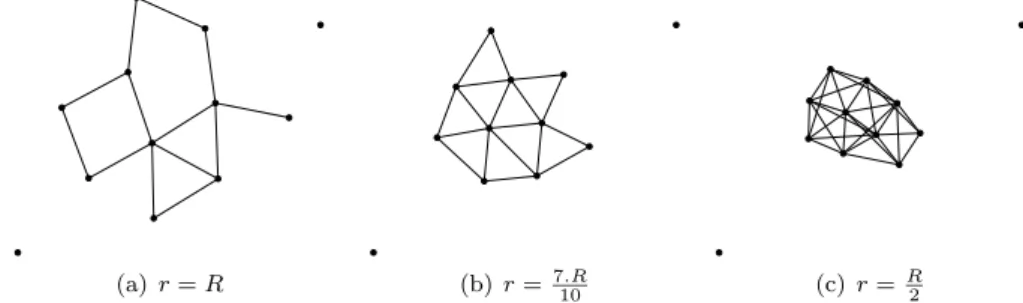
(a) r = R (b) r = 7.R
10 (c) r = R 2
Figure 10: Resulting graph for different value of r. In Fig. 10(a) we plot the resulting graph when r = R. In Fig. 10(b) we plot the resulting graph for r = 7.R
10 and in Fig. 10(c) for r = R
2. In all simulations, we have 10 nodes. Figures are plot in the same scale.
The resulting graph are plotted in Figure 10 at the end of the simulation for 10 moving nodes and different value of r. In Figure 10(a), r = R, in Figure 10(b), r = 7.R10 and in Figure 10(c), r = R
2. These results show that since the distances between nodes are reduced, the resulting graph becomes dense. It is worth noting that the desired range adaptation can be used to provide k-coverage [25] or k-connectivity [9].
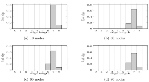
Figure 11 presents the distribution of edge length for different number of nodes when the desired range is r = 7.R
10. We can see from this figure that at least 55% of the edges have a length between [7, 8[ with these simulation setup.
7
Special cases
In this section we present some simulation results for different directions choices in Algorithm 1. We mainly modify Part II of Algorithm 1 to reflect different expansion policy. We focus on two special cases where the direction is chosen depending on the requirements of the coverage application. Both proposition are based on a different direction policy presented in Section 7.1 which is based on the barycenter of RNG neighbors to compute the node destination. Section 7.2 presents the appplication of this direction computation for Point of Interests Coverage and Section 7.3 presents the results for barrier coverage.
0 1 2 3 4 5 6 7 8 0 0.2 0.4 0.6 0.8 edge length % of ed ge (a) 10 nodes 0 1 2 3 4 5 6 7 8 0 0.2 0.4 0.6 0.8 edge length % of ed ge (b) 30 nodes 0 1 2 3 4 5 6 7 8 0 0.2 0.4 0.6 0.8 edge length % of ed ge (c) 60 nodes 0 1 2 3 4 5 6 7 8 0 0.2 0.4 0.6 0.8 edge length % of ed ge (d) 80 nodes
Figure 11: Edge length distribution for different number of nodes. For all simulation R = 10 and r = 7.R10 .
7.1
Barycenter direction
7.1.1 Algorithm description
In this section we have modified the direction computed in Part II of Algo-rithm 1. A node goes toward the barycenter of its RNG neighbors if it has more than one RNG neighbors and goes further than its neighbor if it as only one. Algorithm 2 shows this direction computation.
Algorithm 2MSD (Mobile Sensor Deployment) protocol PartII — Direction computation on nodeu:
1: B(x(B), y(B)) barycenter of RN G(u)
2: x(B) = 1 |RN G(u)| X v∈RN G(u) d(u,v)<R x(v) 3: y(B) = 1 |RN G(u)| X v∈RN G(u) d(u,v)<R y(v) 4:→−∆ = −→ uB ||−→uB||; 5: if((−→∆ ==−→0 && d−
(u) == 0) || (|RN G(u)| == 0)) then
6: Choose a random/predefined direction;
7: end if
8: if(|RN G(u)| == 1) then
9: Go farther than RN G−
(u);
10: end if
In Algorithm 2, B is the barycenter of RN G(u) and node u moves toward this barycenter based on the direction−→∆. If |RN G(u)| = 1, Line 8 of Algorithm 2, node u moves further from this node. The condition on Line 5 of Algorithm 2, is used to get a direction when two nodes are on the same location or if a node does not have an RN G neighbor.
7.1.2 Algorithm properties
Theorem 7 Connectivity: When using Algorithm 2, if at time t = T the graph is connected, ∀t = i, i > T the resulting graph at time t = i is connected.
Proof. The same proof as in Theorem 2 holds, since part II and Part III are independent and the proof of connectivity is done based on Part III of the deployment algorithm.
Let us modify Part III of the algorithm by adding the following lines: [3-0] dopt= {d ∈ [0, dmax] | ∀v ∈ RN G(u), d(unew, v) + νoth× δ < R};
[3-1] if (dopt> d(u, B) )
[3-2] dopt= d(u, B);
[3-3] end if
These modifications are used to restrict the distance covered by node u to the distance d(u, B).
Theorem 8 Oscillation: When using Algorithm 2, if we assume that two nodes cannot have the same location, if at time t = i a node u chooses a direction
−→
∆i6=−→0 and a distance di
opt> 0, at time t = i + δ, if node u chooses a direction ||−−−→∆i+δ|| = −||−∆→i|| then di+δ
opt < diopt for di+δopt > 0.
Proof. The same proof as in Theorem 3 and 4 holds since the point E defined as the end point of the movement of node u in Section 5.2 (for p = 2) is equivalent to the barycenter of RN G(u).
As in Theorem 4, the Oscillation property can only be proved between two points. Moreover, Expansion and Termination properties are not provided by using Algorithm 2.
7.1.3 Simulations
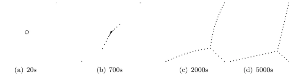
This direction modification is done to show the separation between direction and connectivity and to provide simple example of direction computation that may be useful for specific applications. The figure 12 shows the evolution of the graph when this direction computation is used. In this figure, we do not plot the links between nodes since we have proved that the connectivity is kept. We can see in
(a) 20s (b) 700s (c) 2000s (d) 5000s
Figure 12: Evolution of node’s position and associated graph depending on time. When the node goes toward the barycenter of its RNG neighbors. In this simulation there is 40 nodes with a range of 10 on a square of 100 × 100. Figure 12 that there are nodes located on the corners. This is due to the repelling
direction compute when a nodes as only one neighbor. Based on these nodes that are located on the corner, the other nodes self-organize to form the pattern depicted in Figure 12(d). In our simulations, nodes positions are computed randomly at the beginning of the simulation to avoid overlapping nodes. The random position of each node is within a circle of diameter 1 centered in middle of the field. This explains why in this sample simulation, the upper-right, lower-left and lower-right corners seem to be attractors. The Figure 13 plots some
(a) 8 nodes (b) 30 nodes (c) 60 nodes (d) 80 nodes
Figure 13: Other example of deployments using the barycenter as the direction. This figure plot the resulting graph after 5000s for different number of nodes with a range of 10 on a square of 100 × 100
example of resulting graph when the direction computation is based on the barycenter for different number of nodes. We can see from this figure that the distance between two nodes in the graph is independent from the communication range since nodes only try to be the barycenter of their RNG neighbors. It is also important to notice here that when border effects are not considered (for small number of nodes) the covered area is very close to the one obtained by the initial algorithm (see Fig. 14).
10 15 20 25 30 35 40 0.2 0.3 0.4 0.5 0.6 #nodes % co ve ra ge Intial algorithm Barycenter triangle square hexagon
Figure 14: Coverage results for barycenter direction.
This direction choice is therefore not suitable for maximizing area coverage. It is more appropriate for some barrier coverage since sensors are more likely to form a straight line during the deployment. This is mainly due to the fact that the barycenter of two nodes are in the line joining these two nodes.
The Figure 15 plots the length (for R = 10) and the degree distribution for 60 nodes. This figure shows that compared to the initial algorithm the degree of a node is not bounded and that edge length is uniformly distributed. This
012345678910111213141516171819202122232425262728 0 5 · 10−2 0.1 0.15 0.2 degree % of no de (a) Degree 0 1 2 3 4 5 6 7 8 9 10 0 5 · 10−2 0.1 edge length % of ed ge (b) Edge length
Figure 15: Degree and edge length distribution for 60 nodes. For all simulation R = 10.
figure confirm the fact that barycenter direction is not suitable for maximizing area coverage.
7.2
Point of Interest (POI)
Since whole area coverage may not be necessary, the previous algorithms (Alg. 1 and 1) can be modified to monitor some point of interest in the field [6]. In this section we present the modifications applied to the Algorithm 2 to provide POI coverage. The only modification is done on Line 2 and Line 3, Part II of Algorithm 2. We simply add the following line:
[2] x(B) = 1 |RN G(u)| + 1 X v∈RN G(u) d(u,v)<R x(v) + x(I) [3] y(B) = 1 |RN G(u)| + 1 X v∈RN G(u) d(u,v)<R y(v) + y(I)
where I is the coordinate of a POI. This simple modification can strongly change the shape of the resulting graph. I becomes an attractor. It is important to notice here that Oscillation, Expansion and Termination results cannot be proved. However, since Part II is independent from Part III, connectivity is preserved.
For the POI coverage, we do not use our initial algorithm since we do not need to maximize area coverage. In this case, the straight lines provided by the ’barycenter’ deployment is useful to connect the POI to base station by minimizing the used node. It is worth noting that there may be more than one POI to be monitored and not all but only part of the nodes in the network can be affected to a given POI. Since our deployment protocol preserves connectivity, it is possible to change add/modify a point of interest at any time by a simple regular flooding in the network.
In the simulation results presented in this section we define four POIs in a field of 100 × 100 at coordinate (10, 50), (50, 10), (90, 50) and (50, 90). We also define a node at position (0, 0) as a base station. The starting point of all nodes is in the communication range of the base station. All the nodes have a predefined point of interest randomly chosen at the beginning of the simulation. The base station node is only defined to fit deployment where POIs have to be covered and a connectivity to a fixed based station need to be kept.
Figure 16 plots the resulting graphs for 60 and 80 nodes. Since connectivity is kept, we do not plot edges, instead we plot the sensing range of each node.
(a) 60 nodes (b)80 nodes
Figure 16: POI deployments using the barycenter as the direction. This figure plots the resulting graph after 5000s for different number of nodes with a range of 10 on a square of 100 × 100
Here, the sensing range is equal to the communication range. We can see from these figures that the four points of interest are covered by more than 6 sensors (for 60 nodes). Figure 17 shows that the number of covering node is increasing with the total number of nodes. We can see in Figure 17 that the coverage of a given POI depends on its distance from the starting point of the deployment (here (0, 0)). This is due to the fact that 1/4 of nodes are affected to a given POI and for example 5 = 20/4 nodes are not enough to reach the point (50, 90). We can also see that the number of covering nodes is linearly increasing for each POI. This shows that the number of nodes connecting the base station and a POI (if possible) is independent from the total number of nodes. This property is confirmed by the example of resulting POI coverage in Figure 16.
20 30 40 50 60 70 80 0 5 10 15 #nodes # co ve ri n g n o d es POI (50,10) POI (10,50) POI (90,50) POI (50,90)
Figure 17: Results for POI coverage. This figure plots the number of nodes covering a given POI depending on the total number of nodes in the network.
7.3
Barrier Coverage
Barrier coverage [12, 5] is an important way of covering area especially when considering intrusion detection. Since in Algorithm 2 connectivity is indepen-dent from the direction computation, we can easily modify the direction while
keeping the properties of our algorithm such as connectivity. Unlike in [12] our deployment is focused on maintaining the graph connectivity while providing barrier coverage.
In this section we present the modifications applied to Algorithm 2 to provide self deployment of sensor network for barrier coverage. In our algorithm we consider the barrier coverage as a special case of POI coverage. In barrier coverage, POI are used to define a barrier between the starting points and the POI. Unlike in POI coverage, our aim is not to cover the POI, instead, we want the nodes to be regularly spread out between the starting point and the POI.
The modifications are done based on the POI coverage modifications. We add the following line before the direction computation in Line 1, Part II of Algorithm 2:
[0-1] if (d(u, I) == 0 ) [0-2] Stop node u motion; [0-3] remove POI: I; [0-4] end if
In Line [0 − 1], node u checks if it is above I (I is the POI). If node u is above this POI, node u stops moving and becomes fixed. Moreover to avoid other nodes to concentrate above this POI, node u sends a flooding message in the whole network, since the connectivity is kept, to inform the other nodes that the POI is already covered.
When node u becomes fixed, the other nodes deploy themselves to be above the barycenter of their RNG neighbors. This behaviour of our algorithm pro-vides a dense barrier since sensors will form a line between POIs and the base station. The simulation in Figure 18 presents the resulting graph for barrier coverage when 60 nodes are used and for a single POI defined. These results
(a)(50,50) (b)(50,90) (c) (100,50) (d)(100,100)
Figure 18: Example of deployments for barrier coverage. We only set one POI and a fixed base station at coordinate (0,0). This figure plots the resulting graph after 5000s for different POI coordinates with a range of 10 on a square of 100 × 100 with 60 nodes.
show that our deployment algorithm provides a straight line deployment that becomes a barrier from one defined POI and a fixed based station. When more than one POIs are defined the algorithm has to be modified. When a node reaches its assigned POI, the other nodes that are assigned to this POI try to reach the barycenter of its RNG nodes and we add an attractor which is the segment between the base station and the POI. The Figure 19 plots some ex-amples of deployments where 2 to 5 POIs are defined. In this simulation, 1/5 of the number of nodes are assigned to each POIs to form the barrier. We can see from this figure that the sensors form a straight line between the base station and each POI. Unlike for POI coverage in the previous section, all nodes are
(a)2 POIs (b)3 POIs (c) 4 POIs (d)5 POIs
Figure 19: Example of deployments for barrier coverage with 5 POIs and a fixed base station at coordinate (0,0). This figure plots the resulting graph after 5000s for different POI location and number with a range of 10 on a square of 100 × 100 with 90 nodes.
located between the base station and the POI and thus results in a dense barrier formation when the number of POIs is small (for the same number of nodes).
8
Conclusion
Connectivity is an important property in wireless network and especially in wireless sensor networks. In this paper we provided some distributed and lo-calized algorithm for mobile sensor deployments with connectivity guarantee. Our algorithm is divided into two independent parts. 1) Direction compu-tation. In this part, the direction of the mobile sensor is computed depending on the application requirements. In this paper, we provide three examples of requirements for mobile sensor application deployment. The first deployment tries to maximize the area coverage. We showed that our deployment scheme provides a coverage close to the regular pattern coverage with squares. The second deployment is for Point of Interests (POI) coverage. We showed that the number of nodes involved in the connectivity preservation is independent of the number of node in the network. Therefore increasing the number of nodes, increases the coverage of the POI. Third, we proposed a example of barrier coverage and show that when an end point is defined, the deployment form a line between the starting point (with a fixed base station) and the end point. We also show that increasing the number of node increase the density of the line. 2) Connectivity preservation. In this part, we provided a connectivity preservation scheme to avoid nodes to be disconnected during their deployment. To preserve connectivity, nodes only maintain the connections with a sub-part of its neighbors during the deployment. We chose the Relative Neighborhood Graph since it can be computed locally and it maintains global connectivity.
The independence between the direction computation and the connectivity preservation allows the modification of each part without modifying the other part. The next steps of this work will focus on other connectivity preservation schemes and properties such as k-connectivity or with a degree constraints on each node. We also showed by simulation (for coverage maximization) that the degree of the node is related to the desired edge length. We will thus try to provide a formal relationship between these two assumptions. Moreover, we will try to propose mobile deployments where coverage maximization, POI coverage
and barrier coverage are needed at the same time or depending on the network evolution.
References
[1] X. Bai, S. Kumar, D. Xuan, Z. Yun, and T. H. Lai. Deploying wireless sen-sors to achieve both coverage and connectivity. In MobiHoc ’06: Proceedings
of the 7th ACM international symposium on Mobile ad hoc networking and computing, pages 131–142, New York, NY, USA, 2006. ACM.
[2] M. A. Batalin and G. S. Sukhatme. Spreading out: A local approach to multi-robot coverage. In in Proc. of 6th International Symposium on
Distributed Autonomous Robotic Systems, pages 373–382, 2002.
[3] J. Carle and D. Simplot-Ryl. Energy-efficient area monitoring for sensor networks. Computer, 37(2):40–46, 2004.
[4] J. Cartigny, F. Ingelrest, D. Simplot-Ryl, and I. Stojmenovic. Localized LMST and RNG based minimum-energy broadcast protocols in ad hoc networks. Ad Hoc Networks, 3(1):1 – 16, 2005.
[5] A. Chen, S. Kumar, and T. H. Lai. Designing localized algorithms for barrier coverage. In MobiCom ’07: Proceedings of the 13th annual ACM
international conference on Mobile computing and networking, pages 63–74,
New York, NY, USA, 2007. ACM.
[6] W. Cheng, M. Li, K. Liu, Y. Liu, X. Li, and X. Liao. Sweep coverage with mobile sensors. In IPDPS, pages 1–9, 2008.
[7] A. Howard, M. J. Matari´c, and G. S. Sukhatme. Mobile sensor network deployment using potential fields: A distributed, scalable solution to the area coverage problem. In Proceedings of the International Symposium on
Distributed Autonomous Robotic Systems, pages 299–308, 2002.
[8] J. Jaromczyk and G. Toussaint. Relative neighborhood graphs and their relatives. Proceedings of the IEEE, 80(9):1502–1517, Sep 1992.
[9] A. Kashyap, S. Khuller, and M. Shayman. Relay placement for higher order connectivity in wireless sensor networks. INFOCOM 2006. 25th IEEE
In-ternational Conference on Computer Communications. Proceedings, pages
1–12, April 2006.
[10] O. Khatib. Real-time obstacle avoidance for manipulators and mobile robots. Robotics and Automation. Proceedings. 1985 IEEE International
Conference on, 2:500–505, Mar 1985.
[11] A. Krause, C. Guestrin, A. Gupta, and J. Kleinberg. Near-optimal sen-sor placements: maximizing information while minimizing communication cost. Information Processing in Sensor Networks, 2006. IPSN 2006. The
[12] S. Kumar, T. H. Lai, and A. Arora. Barrier coverage with wireless sensors. In MobiCom ’05: Proceedings of the 11th annual international conference
on Mobile computing and networking, pages 284–298, New York, NY, USA,
2005. ACM.
[13] V. J. Lumelsky and A. A. Stepanov. Path-planning strategies for a point mobile automaton moving amidst unknown obstacles of arbitrary shape.
Algorithmica, 2:403–430, 1987.
[14] S. Poduri, S. Pattem, B. Krishnamachari, and G. S. Sukhatme. Using local geometry for tunable topology control in sensor networks. IEEE
Transac-tions on Mobile Computing, 8(2):218–230, 2009.
[15] S. Poduri and G. Sukhatme. Constrained coverage for mobile sensor net-works. Robotics and Automation, 2004. Proceedings. ICRA ’04. 2004 IEEE
International Conference on, 1:165–171 Vol.1, April-1 May 2004.
[16] D. Pompili, T. Melodia, and I. F. Akyildiz. Deployment analysis in under-water acoustic wireless sensor networks. In WUWNet ’06: Proceedings of
the 1st ACM international workshop on Underwater networks, pages 48–55,
New York, NY, USA, 2006. ACM.
[17] R. Shahidi, M. Shayman, and P. Krishnaprasad. Mobile robot navigation using potential functions. Robotics and Automation, 1991. Proceedings.,
1991 IEEE International Conference on, pages 2047–2053 vol.3, Apr 1991.
[18] D. Simplot-Ryl, I. Stojmenovic, and J. Wu. Energy-efficient backbone construction, broadcasting, and area coverage in sensor networks. Handbook
of Sensor Networks, pages 43–380343–380, 2005.
[19] P. Song and V. Kumar. A potential field based approach to multi-robot manipulation. Robotics and Automation, 2002. Proceedings. ICRA ’02.
IEEE International Conference on, 2:1217–1222, 2002.
[20] I. Stojmenovic and X. Lin. Power-aware localized routing in wire-less networks. Parallel and Distributed Systems, IEEE Transactions on, 12(11):1122–1133, Nov 2001.
[21] G. Tan, S. A. Jarvis, and A.-M. Kermarrec. Connectivity-guaranteed and obstacle-adaptive deployment schemes for mobile sensor networks. In
ICDCS ’08: Proceedings of the 2008 The 28th International Conference on Distributed Computing Systems, pages 429–437, Washington, DC, USA,
2008. IEEE Computer Society.
[22] G. T. Toussaint. The relative neighbourhood graph of a finite planar set.
Pattern Recognition, 12(4):261 – 268, 1980.
[23] M. Younis and K. Akkaya. Strategies and techniques for node placement in wireless sensor networks: A survey. Ad Hoc Networks, 6(4):621 – 655, 2008.
[24] M. Zavlanos and G. Pappas. Potential fields for maintaining connectivity of mobile networks. Robotics, IEEE Transactions on, 23(4):812–816, Aug. 2007.
[25] Z. Zhou, S. Das, and H. Gupta. Connected k-coverage problem in sensor networks. Computer Communications and Networks, 2004. ICCCN 2004.
Proceedings. 13th International Conference on, pages 373–378, Oct. 2004.
Contents
1 Introduction 3
2 Related Work 4
3 Basic idea of our approach 6
3.1 Notations and assumptions . . . 6
3.2 Basic idea . . . 6 4 Protocol description 7 5 Algorithm properties 8 5.1 Connectivity . . . 9 5.2 Oscillations . . . 10 5.3 Expansion . . . 12 5.4 Termination . . . 13 6 Simulation results 13 6.1 Example of networks . . . 14 6.2 Coverage . . . 14 6.3 Covered distance . . . 15 6.4 Graph properties . . . 16 6.4.1 Degree . . . 16 6.4.2 Edge length . . . 16 7 Special cases 18 7.1 Barycenter direction . . . 19 7.1.1 Algorithm description . . . 19 7.1.2 Algorithm properties . . . 20 7.1.3 Simulations . . . 20
7.2 Point of Interest (POI) . . . 22
7.3 Barrier Coverage . . . 23
4, rue Jacques Monod - 91893 ORSAY Cedex (France)
Centre de recherche INRIA Nancy – Grand Est : LORIA, Technopôle de Nancy-Brabois - Campus scientifique 615, rue du Jardin Botanique - BP 101 - 54602 Villers-lès-Nancy Cedex
Centre de recherche INRIA Rennes – Bretagne Atlantique : IRISA, Campus universitaire de Beaulieu - 35042 Rennes Cedex Centre de recherche INRIA Grenoble – Rhône-Alpes : 655, avenue de l’Europe - 38334 Montbonnot Saint-Ismier Centre de recherche INRIA Paris – Rocquencourt : Domaine de Voluceau - Rocquencourt - BP 105 - 78153 Le Chesnay Cedex Centre de recherche INRIA Sophia Antipolis – Méditerranée : 2004, route des Lucioles - BP 93 - 06902 Sophia Antipolis Cedex
Éditeur
INRIA - Domaine de Voluceau - Rocquencourt, BP 105 - 78153 Le Chesnay Cedex (France)
http://www.inria.fr