Interglacials of the last 800,000 years

HAL Id: hal-03259904

https://hal.archives-ouvertes.fr/hal-03259904

Submitted on 14 Jun 2021

HAL is a multi-disciplinary open access

archive for the deposit and dissemination of

sci-entific research documents, whether they are

pub-lished or not. The documents may come from

teaching and research institutions in France or

abroad, or from public or private research centers.

L’archive ouverte pluridisciplinaire HAL, est

destinée au dépôt et à la diffusion de documents

scientifiques de niveau recherche, publiés ou non,

émanant des établissements d’enseignement et de

recherche français ou étrangers, des laboratoires

publics ou privés.

A. Berger, M. Crucifix, D.A. Hodell, C. Mangili, J.F. Mcmanus, B.

Otto-Bliesner, K. Pol, D. Raynaud, L.C. Skinner, P.C. Tzedakis, et al.

To cite this version:

A. Berger, M. Crucifix, D.A. Hodell, C. Mangili, J.F. Mcmanus, et al.. Interglacials of the last

800,000 years. Reviews of Geophysics, American Geophysical Union, 2016, 54 (1), pp.162 - 219.

�10.1002/2015rg000482�. �hal-03259904�

Interglacials of the last 800,000years

Past Interglacials Working Group of PAGES1

1_{See Appendix A}

Abstract

Interglacials, including the present (Holocene) period, are warm, low land ice extent (high sea level), end-members of glacial cycles. Based on a sea level definition, we identify eleven interglacials in the last 800,000 years, a result that is robust to alternative definitions. Data compilations suggest that despite spatial heterogeneity, Marine Isotope Stages (MIS) 5e (last interglacial) and 11c (~400 ka ago) were globally strong (warm), while MIS 13a (~500 ka ago) was cool at many locations. A step change in strength of interglacials at 450 ka is apparent only in atmospheric CO2and in Antarctic and deep ocean temperature. The onset of an

interglacial (glacial termination) seems to require a reducing precession parameter (increasing Northern Hemisphere summer insolation), but this condition alone is insufficient. Terminations involve rapid, nonlinear, reactions of ice volume, CO2, and temperature to external astronomical forcing. The precise timing of events

may be modulated by millennial-scale climate change that can lead to a contrasting timing of maximum interglacial intensity in each hemisphere. A variety of temporal trends is observed, such that maxima in the main records are observed either early or late in different interglacials. The end of an interglacial (glacial inception) is a slower process involving a global sequence of changes. Interglacials have been typically 10–30 ka long. The combination of minimal reduction in northern summer insolation over the next few orbital cycles, owing to low eccentricity, and high atmospheric greenhouse gas concentrations implies that the next glacial inception is many tens of millennia in the future.

1. Introduction

—Interglacials of the Last 800 ka

Earth’s climate of the last 800 ka (1 ka = 1000 years) is the latest stage in a slow cooling that has been in progress for the last ~50 Ma (1 Ma = 1 million years) [Zachos et al., 2008]. During this cooling, ice sheets formed on the Antarctic continent ~40 Ma ago, while thefirst signs of Northern Hemisphere (NH) glaciation appeared much more recently. Only at the start of the Quaternary Period and the Pleistocene Epoch, ~2.6 Ma ago, did alternations between cold glacial periods with ice on the NH continents, and warmer intervals with little or no NH continental ice,first appear, reflected in the appearance of ice-rafted debris [Shackleton et al., 1984; Kleiven et al., 2002] and in enhanced amplitude of cyclicity in benthic oxygen isotopes in marine sediment records (Figure 1) [Lisiecki and Raymo, 2005].

Somewhere between 1.2 and 0.6 Ma ago, weaker cycles with a period of ~40 ka gave way to stronger (greater isotopic amplitude) cycles with a recurrence period closer to 100 ka. This change is known as the Mid-Pleistocene Transition or Revolution. Its exact date is debated, and it is likely that different aspects of climate shifted into their new mode of operation at different times [Mudelsee and Schulz, 1997; Rutherford and D’Hondt, 2000; Clark et al., 2006; Elderfield et al., 2012]. By 800 ka ago, the change in ampli-tude was complete in most records, and glacial cycles with sea level ampliampli-tudes of more than 100 m were occurring, mostly with lengths of the order of 100 ka. The last 800 ka time period also benefits from the enormous progress over recent decades in collecting and analyzing a wide range of continuous climate records from terrestrial sites, marine sediment cores, and the oldest Antarctic ice cores. It is approximately the most recent interval associated with the orientation of the Earth’s magnetic field in the “normal” polarity with the inclination vector pointing north [Shackleton et al., 1990], providing a useful sedimentary demarcation in settings where magnetic reversals are preserved. As an additional motivation, it has also become possible in recent years to run Earth models of intermediate complexity (EMICs) through several glacial cycles, and full Earth system models (ESMs) for a significant range of boundary conditions, including those appropriate for some of the recent interglacials.

Interglacials are the warm, low ice extent (high sea level) end-members of the glacial cycles– although as we shall discuss, the exact definition of an interglacial is not simply stated. We live in such an interglacial. Human actions, increasing the concentration of greenhouse gases in the atmosphere, ensure that our climate will

Reviews of Geophysics

REVIEW ARTICLE

10.1002/2015RG000482

Key Points:

• We have reviewed the occurrence, strength, shape, and timing of interglacials

• Despite spatial variability, MIS 5 and 11 stand out as strong/warm • The current interglacial is expected to

be longer than any of those reviewed

Supporting Information: • Data Set S1 caption • Data Set S1 Correspondence to: E. W. Wolff, ew428@cam.ac.uk

Citation:

Past Interglacials Working Group of PAGES (2016), Interglacials of the last 800,000 years, Rev. Geophys., 54, 162–219, doi:10.1002/2015RG000482. Received 3 MAR 2015

Accepted 17 NOV 2015

Accepted article online 20 NOV 2015 Published online 5 MAR 2016

©2015. The Authors.

This is an open access article under the terms of the Creative Commons Attribution License, which permits use, distribution and reproduction in any medium, provided the original work is properly cited.

become warmer in the next century and remain warm for many millennia to come [Intergovernmental Panel on Climate Change (IPCC), 2013]. This makes particularly pertinent the study of periods in which at least sectors of the Earth system may have been “warmer” than they are currently.

Our understanding of the climate of our current interglacial is good in a static sense: given the boundary conditions (solar irradiance, astronomical character-istics, geography, ice cover, and concen-trations of long-lived greenhouse gases such as CO2) and the resulting radiation

balance of the planet. However, we cannot currently give a satisfactory explanation of how the climate system evolved to this state: why we live in an interglacial at this time, or indeed why we live in an interglacial embedded in 100 ka rather than 40 ka cycles.

Finally the entries into interglacials (and exits from them) are fascinating examples of nonlinear behavior of the Earth system that need to be understood. For these reasons—importance of warm periods, need to understand how our current climate arose, fascinating climate dynamics, and recent availability of significant amounts of data and model simulations—it is timely to review and synthesize existing knowledge about the warm periods (interglacials) of the last 800 ka.

After identifying what an interglacial is, this review aims to summarize the common features and differences between them. This allows us to highlight particular interglacials that may enlighten us about the climate system and to describe current knowledge of the factors that lead into and out of an interglacial. The review ends with a discussion about the likely extent of the present interglacial, both in the absence and presence of human influence on the climate system.

2. Identifying Interglacials

2.1. Nomenclature and History

Terrestrial, marine, and ice core sequences deposited since the intensification of NH glaciation, ~2.6 Ma ago have traditionally been divided on the basis of climate changes inferred from their lithological, biological, and geochemical signature. The fundamental units of this geologic-climate classification [American Commission on Stratigraphic Nomenclature, 1961] are (i) glaciations (or glacials), representing episodes during which extensive glaciers developed, and (ii) interglaciations (or interglacials), representing episodes during which the climate was incompatible with the wide extent of glaciers. Further subdivisions include stades (stadials) and interstades (interstadials), reflecting secondary advances and recessions or standstills of glaciers, respectively.

The term “interglacial” derives from the position of temperate-climate sediments interbedded between glacial sediments [Heer, 1865; Geikie, 1874]. In the higher midlatitudes of Europe and North America the concept of an interglacial as an interval of time during which conditions were at least as warm as the present interglacial (Holocene) was traditionally based onfloral evidence, indicating the development of temperate deciduous forest [e.g., Jessen and Milthers, 1928; Fairbridge, 1972; Woillard, 1978; West, 1984; Gibbard and West, 2000]. By comparison, the term interstadial has been used to describe a period that was either too short or too cold to allow the development of temperate deciduous forest. Similar distinctions were also adopted for faunal evidence [e.g., Coope, 1977].

Figure 1. Benthic oxygen isotope stack for the last 5 Ma [Lisiecki and Raymo, 2005]. Oxygen isotopes in benthic foraminifera represent a combination of changes in the oxygen isotope content of the water (dominated by ice volume) and deepwater temperature. This plot shows the onset of cyclicity, when Northern Hemisphere ice started to wax and wane, at ~2.6 Ma ago (arrow marks the official start of the Quaternary), and the strengthening and lengthening of cycles across the mid-Pleistocene transition (horizontal bar).

In deep-sea sediments, the terms glacial and interglacial werefirst applied to even- and odd-numbered oxygen isotope stages, respectively, defined by variations in the oxygen isotope ratio (δ18O) in planktonic foraminifera andfirst thought to reflect changes in sea surface temperature [Emiliani, 1955]. However, the concept of a marine isotopic stratigraphy is based on the principle that changes in the oxygen isotopic composition of the oceans primarily arises from changes in the volume of ice stored on the continents [Shackleton, 1967] and that given the slow mixing of the deep ocean, such a signal would be global on timescales of thousands of years. Shackleton and Opdyke [1973] proposed the formalization of Marine Isotope Stages (MIS) 1–22, using the δ18O in foraminifera in core V28-238 from the Eastern Equatorial Pacific, a practice which has been gradually extended over the entire Pleistocene, Pliocene, and beyond. Marine isotope stages may be further divided into substages (e.g., MIS 5 into 5a-5e [Shackleton, 1969]), characterized by local minima and maxima inδ18O values known as marine isotopic events [Prell et al., 1986], such that MIS 5a contains event 5.1, MIS 5b contains event 5.2, and so on. The decimal event notation has occasionally been used to denote substages, but the two systems are not interchangeable. An event refers to a point in time rather than an interval; in a detailed record there will be space between successive events, whereas substages have boundaries and togetherfill the stratigraphic record and the time that it represents [Shackleton, 2006]. To avoid confusion, please note that we use a recently recommended substage nomencla-ture [Railsback et al., 2015], which contrasts with some literanomencla-ture usage, particularly for MIS 9 and MIS 15. A major development in the understanding of the correspondence between marine and terrestrial stages was the realization that the Eemian (Last) Interglacial of northwest Europe is not equivalent to the whole of MIS 5, but rather approximates to a substage (MIS 5e) within it [Shackleton, 1969]. In line with the terrestrial evidence, other isotopically depleted marine substages corresponded to interstadials associated with the same interglacial complex (so that MIS 5c and 5a would broadly correspond to the Amersfoort/Brörup and Odderade interstadials, respectively, of the northwest European stratigraphy). Joint foraminiferal isotopic and pollen analyses from marine sequences have not only confirmed such correlations but also showed that the marine and terrestrial stage boundaries are not necessarily time parallel, reflecting geographical asynchroneity and differences in response times of, e.g., vegetation and ice [Sánchez Goñi et al., 1999; Shackleton et al., 2002, 2003; Tzedakis et al., 2004].

2.2. Definition of Interglacial

The population of interglacials must be defined before any attempt is made to discuss their individual charac-teristics, including the statistics of their timing and spacing. Given that interglacial complexes (odd-numbered Marine Isotope Stages, such as MIS 5, but excluding MIS3 which is not now considered to include an interglacial period) contain a number of temperate intervals within them, a crucial question is how to categorize intergla-cials and distinguish them from interstadials. In some conceptual models [Parrenin and Paillard, 2003], the climate system occupies (and jumps between) a glacial and deglacial (or interglacial) state, with different governing equations in each. While a bifurcation structure may indeed be relevant for describing the dynamics of glacial-interglacial cycles, identifying it from the available paleo-observations is complex [Imbrie et al., 2011]. Distinguishing interglacial from interstadial climates is nonetheless important, not only on formal stratigraphic grounds but also in climatic context. Though temperate in climatic signature, interstadials are still part of a glacial world with excess ice in the Northern Hemisphere outside Greenland. Thus, for example, the Amersfoort/Brörup and Odderade interstadials in northwestern European nomenclature (roughly MIS 5a and 5c) are part of the Early Glacial (MIS 5d-5a) in this region, which reflects not only their stratigraphic position but also their overall climatic character compared to the Eemian.

Central to any definition of an interglacial is the choice of an appropriate criterion that can be applied consis-tently through time. A number of approaches are possible, each with inherent advantages and disadvantages (Table 1). A recurring issue is that distinctions between interglacials and interstadials depend on the metric used. It is desirable that whatever metric is chosen has global significance, such that interglacials are phenomena that can be considered widespread (probably of global extent), even if their regional expression is neither globally uniform or synchronous. Some definitions that have been used are based on temperature. Temperature records exist at many sites but are essentially local, and therefore, the definition of an interglacial based on temperature would vary according to the location. This will remain the case until there are sufficient data with accurate chronologies, such that some kind of global average temperature can be constructed across multiple glacial/interglacial cycles. Only recently has afirst such reconstruction [Shakun et al., 2012; Marcott et al., 2013] become available for the last 22 ka and none is available for earlier interglacials.

We might also be tempted to define interglacials on the basis of the external forcing. At the multimillennial timescale, the dominant external forcing of Earth’s climate is the astronomical forcing. This drives the climate system dynamics which, lead, for example, to variations in atmospheric CO2concentration and in the mass of

the ice sheets. These in turn may be viewed as feedbacks, or as“internal” forcing factors of the atmospheric and oceanic conditions all over the globe. Increased concentrations of CO2, in particular, are a characteristic

of interglacials. However, the relationships between astronomical forcing, CO2and the mass of continental

ice are nonlinear and complex. In particular, eccentricity, often cited as a possible origin of the 100 ka periodi-city characteristic of glacial-interglacial cycles does not appear in the spectrum of regional insolation changes; it merely modulates the amplitude of insolation changes. Combinations of obliquity and precession predict the occurrence of some interglacials [Kukla et al., 1981], but as longer paleoclimate records have appeared, it has become clear that such simple formulae do not correctly predict the full roster observed in the data. It is therefore not currently practical to use astronomical forcing to define interglacials. As discussed earlier, interglacials have been defined as episodes during which global climate was incom-patible with the wide extent of glaciers [American Commission on Stratigraphic Nomenclature, 1961]. While remembering that there is still a large volume of ice in Antarctica during every interglacial, this nonetheless

Table 1. Comparison of Different Approaches to De_{fining Interglacials}a

Definitions Advantages Disadvantages

Conceptual change of state Clear and mechanistic Such a bifurcation may not exist Lack of objective criteria to recognize such a

bifurcation from the existing records “As warm or warmer than the Holocene” Unambiguous in that a demarcation value is set

(e.g., Holocene peak)

In absence of sufficient data to calculate global mean temperature, definition will vary with location. With this definition, no interglacials between 800 and

450 ka ago Fixed threshold (similar to above, but cutoff

value is not determined by Holocene values)

Unambiguous for given metric Depends on metric used (e.g., temperature, sea level, and CO2).

Depending on where threshold is set, it can exclude “cool” interglacials or could include “interstadials”

(e.g., MIS 5a and 5c)

With specific reference to Antarctic records, depends on whether“overshoots” are included in the interglacial

(see section 7.1) Varying threshold, for example, different pre-MBE

versus post-MBE values, or one for each g-ig cycle

If amplitude of signal is genuinely nonstationary when subjected to similar controls, then this

method addresses that.

Depends on metric used (e.g., temperature, sea level, and CO2).

Subjective choice of time period over which threshold can change—makes unproven assumption about

nonstationarity. (alternatively, segments of time series are

normalized and afixed threshold, e.g., one

standard deviation is applied across) _{With specific reference to Antarctic records, depends} on whether“overshoots” are included in the interglacial

(see section 7.1) Interglacial defined as the interval following a

glacial termination

Good for calculating repeat times of g-ig cycles Shifts problem to defining what a termination is. Interglacial defined as the most prominent peak(s)

within each odd-numbered marine isotopic complex

Allows for more than one interglacial within one complex

Depends on metric used (e.g., temperature, sea level, and CO2).

Makes an unwarranted assumption that original numbering system satisfactorily defines

interglacial recurrence. Interglacials are characterized by absence of NH

ice outside Greenland; different interglacials must be separated by lowering of sea level below a set threshold.

Uses a metric (global sea level/ice volume) that integrates global climate effects

Uncertainties with sea level reconstructions Consistent with stratigraphic concepts Subjective choice of remaining NH ice that can be

tolerated and of ice volume increase to separate interglacials.

Allows for more than one interglacial within one complex

a_{It should be noted that some of these definitions are also appropriate for estimating interglacial duration. The difference, however, is that the identification of}

emphasizes that the fundamental concept underlying the terminology of an interglacial is that of low continental ice volume, a consequence of integrated global climate effects, which would also be observed as high sea level or less positive seawaterδ18O. This is in line with early definitions of interglacials based on the marine transgression [e.g., Harting, 1874]. The slow response of ice sheets would mean that the sea level highstand or isotopic minimum may be attained relatively late compared to increases in warmth or climate forcing. Here we clearly distinguish the use of such values to define whether an interglacial is occurring, from any measure used to define when the interglacial starts and ends. As an example, for the current interglacial, sea level close to present, a value we might use to define MIS 1 as an interglacial, occurs as late as ~ 7–8 ka ago. However, having determined that an interglacial is occurring, its start can be defined in other ways [Walker et al., 2009].

A eustatic, or global mean, sea level curve would therefore provide a useful measure to address this issue, but in practice direct sea level determinations are often complicated by local isostatic and gravitational effects and dating uncertainties, are discontinuous, and only cover the most recent part of the record [e.g., Thompson and Goldstein, 2006]. Theδ18O from benthic foraminifera is sometimes used as a sea level proxy, but it is overprinted by local deepwater temperature and hydrographic effects, which can obscure the glacioeustatic signal [Chappell and Shackleton, 1986; Skinner and Shackleton, 2005]; averaging many globally distributedδ18O_benthicrecords as in the stacked record of Lisiecki and Raymo [2005] (hereafter referred to as LR04) does however remove some of the regional variability. Various approaches to isolate the sea level component ofδ18Obenthic[Shackleton, 1987; McManus et al., 1999; Shackleton, 2000; Waelbroeck et al., 2002]

have been attempted, but until recently none of them have been extended to cover the last 800 ka. A mod-eled sea level curve by Bintanja and van de Wal [2008] extends over the last 3 Ma but depends on uncertain assumptions about deepwater temperatures and their coupling with atmospheric temperatures. A record using shallow-infaunal benthic foraminifera to deconvolve deepwater temperatures (using Mg/Ca ratios) and theδ18O of seawater (δ18O_sw) over the last 1.5 Ma has recently become available from Ocean Drilling Program (ODP) site 1123 on the Chatham Rise, east of New Zealand [Elderfield et al., 2012]. With hydrographic effects considered minimal at this site, theδ18Oswprovides an important insight into ice volume changes

over this interval, although the propagated error of ±0.2‰ in calculated δ18Oswestimated by Elderfield

et al. [2012] means that the uncertainty is ±20 m sea level equivalent. A continuous sea level reconstruction based on planktonicδ18O records and a hydrological model for the Red Sea is available for the last 520 ka [Rohling et al., 2009]. A related method covering a longer time period, using a hydrological model for the Mediterranean [Rohling et al., 2014], gives a further useful overview, but with a large propagated uncertainty in sea level, similar to that of Elderfield et al. [2012]. Finally, recent work [Shakun et al., 2015] has used a global compilation of paired planktonicδ18O and sea surface temperatures in an attempt to deduceδ18O of surface seawater, interpreted to reflect mainly ice volume and sea level. However, it is hard to use this record to compare the strength of interglacials because the authors had to make a correction for a long-term trend, believed to be unrelated to sea level.

Given that the LR04 stack is affected by deepwater temperature and hydrographic effects of variable influence through time, we first examine those records where the sea level component has been (mostly) isolated. The ODP Site 1123 [Elderfield et al., 2012], the Red Sea/Mediterranean [Rohling et al., 2009, 2014], and the detrended surface seawater stack [Shakun et al., 2015] records all suggest that within the uncer-tainties of the reconstructions (±20 m), highstands during the most prominent isotopic substages of the last 800 ka reached a level similar to present (Figure 2). Assuming that the East Antarctic ice sheet was not significantly smaller than today, this observation points to a more specific definition of an interglacial as an interval within which the distribution of Northern Hemisphere ice resembled the present (0 ± 20 m), i.e., there was little Northern Hemisphere ice outside Greenland, with periods of significantly greater ice volume (sea level passing below approximately 50 m compared to present) before and after the interglacial period. The second half of the definition is required in order to separate periods of interglacial character that are interrupted by clearly glacial conditions. However, it has consequences for the number of interglacials in MIS 15 and 7. The distinction between an interglacial and an interstadial under this definition lies in the absence/presence of significant Northern Hemisphere ice outside Greenland. An example of this distinction is MIS 5. Evidence from the Norwegian Sea and western Scandinavia indicates ice-free conditions during the Eemian (interglacial), but expansion of mountain glaciers during the Amersfoort/Brørup (MIS 5c) and Odderade (MIS 5a) interstadials leading to increased background values

in the relative abundance of ice-rafted detritus in the Norwegian Sea during these intervals [Baumann et al., 1995]. Tzedakis et al. [2009] assigned an interglacial status to the most promi-nent temperate (low δ18O) interval within each odd-numbered marine isotope stage of the LR04 benthic δ18_{O stack [Lisiecki and Raymo, 2005]}

(with the exception of the historical artifact of MIS 3). On this basis, MIS 5e, 9e, 11c, 13a, 17c, and 19c (and by default MIS 1) are unambiguously the most prominent intervals within each MIS (Figure 2), but choosing the most prominent interval in MIS 7 and MIS 15 is difficult. Yin and Berger [2010, 2012] chose a similar set of interglacials to simulate, using the expectation of a 100 ka cycle to justify including MIS 7e but not 7a-7c, and including MIS 15a but not 15e. Using our sea level definition, MIS 7a-7c and 7e, and also MIS 15a and 15e are all equally prominent within their respective stages, and as we do not assume a particular periodicity, they are all included in our intergla-cial roster, which therefore comprises MIS 1, 5e, 7a-7c (as a single interglaintergla-cial), 7e, 9e, 11c, 13a, 15a, 15e, 17c, and 19c.

Although a definition based on sea level, as we have suggested, is attractive in its simplicity, its application is hampered by uncertainties that remain in the values of sea level provided by indirect but continuous methods. In particular, direct sea level evidence suggests [Dutton and Lambeck, 2012; Kopp et al., 2013] that sea level during MIS 5e was higher than present. However, the (ODP 1123) derived sea level record [Elderfield et al., 2012] places the MIS 5e highstand at the edge of the lowest range of our proposed threshold ( 20 m), and at a similar level in MIS 5a, with MIS 5c higher than both (Figure 2). Had we only the ODP1123 data [Elderfield et al., 2012], then MIS 5a and MIS 5c would have been identified as interglacials on a par with MIS 5e, but we use knowledge from other sea level data sets [Dutton and Lambeck, 2012; Grant et al., 2012; Kopp et al., 2013] to distinguish MIS 5e as an interglacial and MIS 5a and 5c as interstadials. This, however, casts doubt on the reliability of the reconstruction in earlier periods (especially before 450 ka ago) when alternative sea level evidence is weaker. Given this uncertainty, we also test the sensitivity of our interglacial assignments by using simple thresholds in the uncorrected benthic oxygen isotope record (in this case the LR04 stack [Lisiecki and Raymo, 2005]), and in the ice core record of CO2(chosen as a global-scale indicator

which, together with ice volume/extent, affects the global radiative forcing).

Our sensitivity studies with the LR04 benthic isotope stack [Lisiecki and Raymo, 2005] would produce the same set of interglacials for any threshold between 3.5 and 3.73‰ (to qualify as an interglacial, values lower than the threshold must be achieved). Any threshold set lower than 3.5‰ would exclude first MIS 17c and very quickly all other stages except MIS 1, 5e, 9e, and 11c. At thresholds higher than 3.73‰, several other stages, starting with MIS 5c, would become interglacials. The very wide range of thresholds (3.5–3.73‰) that lead to the same answer suggest that this solution is robust, i.e., that new data are unlikely to make it obsolete.

We need also to assess the criterion for how deep the surrounding glacials must be to decide that a peak qualifies as a separate interglacial. Using LR04, it would in theory be possible to set a second threshold

Figure 2. Definition of interglacials based on sea level. (top) δ18O of benthic foraminifera in the LR04 stack [Lisiecki and Raymo, 2005]; (bottom) probability maximum Red Sea relative sea level [Rohling et al., 2009] (orange line); and deconvolvedδ18O of seawater [Elderfield et al., 2012] (grey line). Marine Isotopic substages of interglacial status are indicated (as well as interstadials MIS 5a and 5c). Note that there is some confusion in the literature about the lettering of substages in MIS 9 and 15. Here we use the substage numbering recommended in a recent paper [Railsback et al., 2015], such that the oldest substages in MIS 9 and 15 are 9e and 15e. This contrasts with the usage in some recent papers [Tzedakis et al., 2012b]. Dashed lines mark values discussed in the text that might be used in the definition of interglacials.

for the depth of the valley between interglacials, such that MIS 13 and 15 are separate interglacials, while MIS 7a-7e and MIS 15a-15e each form single very long interglacials. However, the range of values for such a second threshold is very narrow (~0.1‰), suggesting that it has no robust validity. In addition, it would imply inclusion in an interglacial of isotopic values (during MIS 7d and 15b) that are generally characteristic of periods that are clearly part of the glacial world. Afinal argument against this solution is that two of the derived sea level records [Elderfield et al., 2012; Shakun et al., 2015] place sea level lower in MIS 7d than in MIS 14. Thus, unless we are willing to describe MIS 13–15 as a very long continuous interglacial, we are forced to set the threshold such that MIS 7ac and 7e (similarly 15a and 15e) are separate interglacials.

As afinal sensitivity study, we investigate the ice core CO2record [Lüthi et al., 2008; Bereiter et al., 2015];

because of its importance as a radiative forcer at global scale, CO2may plausibly be one of the controlling

factors on interglacial strength in a range of other records (see section 6.7). If the threshold is 260 ppm or higher, only one interglacial (MIS 19) is recognized before MIS 11. However, as the threshold is lowered other interglacials qualify: by 250 ppm, all the interglacials in our roster (including 7c and 15a) have qualified, with the exception of MIS 17c. Periods of clearly interstadial nature in other records get drawn in for lower thresholds, starting with MIS 5a. The low values of CO2in MIS 17c were already noted [Lüthi et al., 2008]

and persist even in the revised data set recently published [Bereiter et al., 2015]. Perhaps most importantly for this sensitivity study, there is again no reasonable criterion using CO₂that qualifies MIS 13a as an intergla-cial without also qualifying MIS 7ac and 15a as separate interglaintergla-cials.

The scheme we have used allows for the occurrence of more than one interglacial within the same complex and does not require an interglacial to follow a traditionally numbered glacial termination. Only a definition that insists on a minimum temporal spacing (of order 100 ka) between interglacials could force a more traditional list of interglacials. While we recognize that the definition applied here will lead to some inconsis-tency in relation to traditional nomenclature, we feel it is justified by its objectivity and robustness against a range of definitions and thresholds; the traditional assumptions on the other hand will lead to misleading conclusions about the spacing and timing of interglacials. It is important to reiterate that this is a working definition based on a global metric and as such it has global stratigraphic significance. Interglacial stages may continue to be defined in local contexts using local signals (e.g., local temperature or forest develop-ment), but they do not carry general applicability. One cautionary note to add is that our definition is clearly dependent on the context of the last 800 ka and would not necessarily be suitable for the early Quaternary, even though we recognize from benthic isotopes that periods with interglacial character existed then, nor for earlier periods containing alternations of icy and ice-free intervals.

3. Methods

Before attempting to assess the nature, intensity, and timing of interglacials, it is necessary to establish and summarize the main methods used to measure interglacial climate characteristics, to place them on an age scale, and to model the processes involved.

3.1. Stratigraphy and Chronology

Regardless of what definition is adopted for an interglacial, the study of past interglacials must be underpinned by a robust stratigraphy and chronology. Comparing climate signals in different archives is challenging and requires precise stratigraphic correlation of marine, ice, and terrestrial records, including those providing infor-mation about sea level and atmospheric composition. Study of the initiation, termination, and duration of interglacials as well as rates of processes is entirely dependent on the accuracy of the timescale. The age model controls the rate, shape, and duration of interglacial periods and absolute ages are needed to discuss the phasing of proxies relative to astronomical forcing. Sampling frequency as well as chronological precision can affect the degree of variability and peak values (amplitude) of the interglacial signal.

The long ice core records have relied mostly on the Antarctic Ice Core Chronology 2012 (AICC2012) based on information from several ice cores [Bazin et al., 2013], and its predecessor, the European Project for Ice Coring in Antarctica (EPICA) Dome C, third generation (EDC3) chronology that was derived by inversion of a snow accumulation and mechanical iceflow model using a set of independently dated horizons (age markers) along the core [Parrenin et al., 2007]. Note that all ages shown infigures in this paper are nominally relative to 1950 as present. The uncertainty of the EDC3 age model is estimated to be ±3 ka at 100 ka ago and

increasing to ±6 ka from 130 ka to the base of the core. AICC2012 [Bazin et al., 2013] shows only small differ-ences from EDC3 and is well within the quoted age uncertainty. The duration of the last four interglacial per-iods is not affected by more than 5% using AICC2012 instead of EDC3 [Bazin et al., 2013]. One powerful alternative method for developing ice core chronologies is orbital tuning of the O₂/N₂ratio to local insolation forcing [Bender, 2002; Kawamura et al., 2007]. This method has the advantage that it dates the ice (which holds the climate signal), rather than the enclosed air, which can be considerably younger because the air bubbles close only at depths of typically 60–100 m). With an assumption that O2/N2is in phase with local

summer insolation, this method provides a link to absolute ages; however, the precision of this assumption has been questioned [Landais et al., 2012]. Vostok O2/N2data are included in AICC2012 as one component of

the age model, but the Dome Fuji (DFO2006) age model relies mainly on this tuning, and a smaller estimated uncertainty (up to 2.5 ka) is quoted. Comparison of EDC3 and Dome Fuji chronologies reveals reasonable agreement for the last 350 ka (within the estimated uncertainty of EDC3, but not always within the uncer-tainty quoted for DFO2006).

Most deep-sea records are dated by correlating benthicδ18O signals to the LR04 stack [Lisiecki and Raymo, 2005]. The LR04 stack is tuned to the output of an ice volume model [Imbrie and Imbrie, 1980] that, in turn, is driven by insolation, assumingfixed response times. The estimated error for LR04 is ±4 ka for the past million years. One of the caveats associated with the LR04 timescale is its reliance on assumptions associated with astronomical forcing of climate. The depth-derived ages of Huybers and Wunsch [2004] are almost free of such assumptions but are estimated to be accurate only to within ±9 ka. The differences between LR04 and other age models fall within the uncertainties of these error estimates (Figure 3).

LR04 and EDC3 or AICC2012 are well aligned with each other although Antarctic temperature changes consistently lead LR04δ18O by an average of 3 ka. The deep-sea temperature component of the benthic δ18_{O signal, as estimated by Mg/Ca, significantly leads the δ}18_O

seawater signal [Elderfield et al., 2012]

Figure 3. Comparison of proxy records on independent timescales. LR04 (blue): benthic_δ18O stack [Lisiecki and Raymo, 2005]; HW04 (green): benthic_δ18O stack on a depth-derived timescale [Huybers and Wunsch, 2004]; EDC3 (lime green):_δDiceon EDC3 timescale [Parrenin et al., 2007]; Dome Fuji (black):_δ18O_ice on DF06 timescale based on O₂/N₂tuned to local insolation [Kawamura et al., 2007]; 1123 (orange): Deep-sea temperature at site ODP1123, SW Pacific [Elder_{field et al., 2012].}

(see discussion below) and agrees closely with the timing of Antarctic temperature change (Figure 3). This likely reflects the late response of ice volume compared to temperature in the benthic δ18O signal. The lead of warming Antarctic and deep-sea temperatures over (NH) ice volume change underscores the problem of how to define the start of interglacial periods because the early warming may not be considered to be part of the interglacial period if defined by ice volume reduction.

Speleothems and corals provide an opportunity for absolute dating of the timing of terminations [e.g., Cheng et al., 2009] and the duration of interglacials by radiometric U series dating, and to determine the phasing of climate change relative to insolation forcing. If age markers from speleothems can be identified as unequivo-cally synchronous to features in ice cores and/or marine sediment cores, then the speleothem chronology can be exported to other archives [e.g., Barker et al., 2011; Grant et al., 2012] and used to evaluate the accuracy of independent chronologies. Full use of such methods awaitsfirm proof that rapid jumps in local speleothem δ18_{O are synchronous with rapid jumps in ice core temperature or atmospheric methane and marine sea surface}

temperature (SST) records. Assumptions of this nature have been disputed [e.g., Blaauw et al., 2010]. Barker et al. [2011] placed the EPICA Dome C (EDC) record on a“Speleo-Age” timescale for the last 400 ka by first differ-entiating the AntarcticδD record, according to a conceptual model of interhemispheric millennial tempera-ture change, to produce a synthetic Greenland record, and then correlating cold events in Greenland with “weak monsoon events” in the detrended speleothem δ18_{O record. The ages agree to within ±2–3 ka with}

EDC3 from present to MIS 11 where the difference increases to 5 ka. A similar approach has been applied to Iberian Margin sediments where planktonicδ18O and SST have been used to synchronize millennial-scale events among marine sediment core, Antarctic ice core, and speleothem records [Barker et al., 2011; Hodell et al., 2013]. Differences between the speleo-synchronized and LR04 age models from the Iberian Margin are less than ±5 ka for the last 400 ka.

While speleothem records can be radiometrically dated, the age models of other long terrestrial records have been derived by tuning lithostratigraphical or biostratigraphical variations to an astronomical target (which may be a local insolation target) or to marine records [Prokopenko et al., 2006; Tzedakis et al., 2006; Melles et al., 2012; Torres et al., 2013]. While this can be done rather precisely, it involves assumptions about synchroneity that could be in error by several thousand years. Unless these assumptions can be tested (for example, through the use of pollen in marine cores, of tephra layers that can be shown to have the same origin, or through the use of dated paleomagnetic boundaries), it is impossible to assess the phasing of change between different processes during relatively rapid changes that occur at terminations in particular.

The accuracy of timescales directly influences our interpretations of the causes of interglacial periods. For exam-ple, the errors associated with the ages for the onset and end of an interglacial period (regardless of defining criteria) are large relative to the accuracy of astronomical solutions, which we take to have no error for the last 800 ka. The absolute chronological error (of order ±5 ka for ice cores and marine records) is also large relative to the duration of interglacial periods, which ranges from ~10 to 30 ka. The age uncertainty (about one quarter of a precession cycle) provides considerable leeway in interpretation of how the onset and end of interglacials align with astronomical forcing, underscoring the importance of reducing chronological error in the future.

3.2. Proxies

Temperature, greenhouse gas (GHG) concentrations, and ice volume (sea level) have been the three reconstructed climate parameters used most often for studying past interglacial periods, although changes in the hydrologic cycle are also important especially at low latitudes and changes in ocean circulation are also highly relevant. Clearly, it is not appropriate here to review all the methods used in paleoclimate recon-struction; however, we briefly summarize the main methods used to derive the records that appear most often in this paper.

In the polar regions, temperature is derived from the ratios of water isotopes (δ18O,δD) in ice cores. This has a strong physical basis as a temperature proxy [Jouzel et al., 1997], but there remains uncertainty about its calibration, particularly for higher temperatures [Sime et al., 2009]. Additional methods to constrain tempera-ture in ice cores have been used [e.g., Buizert et al., 2014] in Greenland ice cores, but so far the water isotopes are the only method used to reconstruct temperatures in the long Antarctic ice cores that extend through several glacial cycles. SSTs are estimated from marine sediment cores using a range of geochemical and biological proxies: fossil assemblages (using foraminifera, coccolithophores, radiolarians, diatoms, or dinocysts), alkenone, and other biomarkers (Uk37, Uk′37, TEX86), Mg/Ca ratios and “clumped” isotopologs of carbon and oxygen.

Each of these methods comes with uncertainty about calibration and about the precise interpretation of the proxy (for example, whether it indicates an annual or seasonal signal). Where methods have been compared, discrepan-cies are found in some regions [Nurnberg et al., 2000; de Vernal et al., 2006; de Garidel-Thoron et al., 2007]. This means that it is difficult to construct consistent spatial time slices of absolute temperature. However, the relative signal within a single proxy at a single site should be much more reliable, so that anomaly data can be used with some confidence to assess the relative strength of different interglacials, or the timing of maxima and transitions at a given location. For terrestrial sites, pollen assemblages may sometimes be used to estimate temperature; many other commonly described terrestrial proxies are influenced by factors other than temperature.

GHG concentrations (particularly, CO₂and CH₄) for the last 800 ka can be determined directly from measure-ments in the air within ice cores [e.g., Loulergue et al., 2008; Lüthi et al., 2008]. The uncertainty in the concentra-tions measured in this way is very small (a few parts per million for CO2and about 10 parts per billion for CH4),

although methodology is important for obtaining correct values, especially in deep ice [Bereiter et al., 2015]. However, in the cores for which old ice is available, there is an inherent limit to the resolution (of several centuries), and an uncertainty in the age relative to the temperature proxy in the same core, because of changes in delta age, the age difference between the ice and the younger air that diffuses from the surface and is trapped within the ice matrix only at depth [e.g., Parrenin et al., 2013]. CH4changes result from changes in

wetlands in the tropics and high northern latitudes and thus are often used as an indicator in the gas phase of the timing of Northern Hemisphere and tropical climate change relative to other signals.

Estimates of relative sea level change at individual sites and dates can be made using a range of methods (already partly discussed in section 2.2). While dated corals are of particular importance, to obtain a continuous (over multiple glacial cycles) and global, eustatic, sea level record, marine sediments remain important. Theδ18O of benthic foraminifera is affected not only by changes in continental ice volume but also by deepwater tem-perature and local hydrographic (water mass) changes. On timescales significantly greater than the mixing time of the oceans (103years), theδ18Ocalcitesignal represents changes in the mean state of the“global ocean” as

local/regional hydrographic changes that exist in the ocean are diminished [Shackleton, 1967; Imbrie et al., 1984; Skinner and Shackleton, 2006]. If an independent estimate of temperature is derived, the seawaterδ18O component (i.e.,δ18Oseawater) of the benthicδ18O signal can be calculated. As discussed in section 2.2, one

approach has been to stack benthicδ18O records assuming that local and regional hydrographic signals are aver-aged out, thereby leaving the common globalδ18O signal [Imbrie et al., 1984; Prell et al., 1986; Lisiecki and Raymo, 2005]. In reality, however, the relative contributions of temperature and ice volume still remain unconstrained in a stacked record. Another approach has been to measure benthicδ18O in cores from regions where deepwater temperature is close to freezing [e.g., Labeyrie et al., 1987]. Others have attempted to modelδ18O_seawaterand sea level from the benthicδ18O stack [Bintanja et al., 2005; Bintanja and van de Wal, 2008] or use a sea level transfer function to convert benthicδ18O to relative sea level equivalent [Waelbroeck et al., 2002]. Mg/Ca ratios of forami-nifera have the potential to reconstruct temperature and, when combined with foramiforami-niferalδ18O measure-ments, provide an estimate of changes in theδ18O of seawater [Elderfield et al., 2010, 2012]. This approach was taken to deconvolveδ18O_seawaterand deepwater temperature at Site ODP1123 in the deep SW Pacific. A completely separate approach for obtaining a continuous (albeit local, and therefore relative) sea level record has been used in a series of papers using marine cores from the Red Sea. This relies on an assumption that δ18

O in foraminifera in these cores is controlled mainly by changes in salinity induced by evaporation, whose influence varies depending on the depth of seawater above a shallow sill that controls exchange with the open ocean. The Red Sea records so far extend only to just over 500 ka ago [Rohling et al., 2009], although a longer record using a similar method for the Mediterranean has been published recently [Rohling et al., 2014]. Different sea level estimates are compared in Figure 2.

3.3. Models

A range of different types of model has been used to study past interglacials. Experiments can be carried out with a range of underlying purposes, for example: testing models that are used to simulate the present and future climate, understanding the dynamics of termination and inception of glacials (i.e., the start and end of interglacials), or understanding the whole dynamics of glacial-interglacial cycles.

By far the most common approach is to carry out snapshot simulations of particular time slices, using models ranging from full ESMs and atmosphere–ocean general circulation models (GCMs), in some cases identical to those used to study present and future climate, through to EMICs. The majority of such simulations have been

conducted for specific time periods in the last interglacial (LIG), in particular under the Paleoclimate Model Intercomparison Project (PMIP)3 exercise [Lunt et al., 2013], which focused on time slices at 130, 128, 125, and 115 ka. Such simulations are driven by boundary conditions distinct from those of the Holocene. For most interglacial simulations, ice sheet extent is assumed similar to that of today, as are other components such as vegetation and aerosol concentration. Therefore, the main changes are in astronomical parameters (which can be calculated precisely) and GHG concentrations (which are derived from ice core data); these can be modified as appropriate for the time period under study. A very few studies have carried out snapshots for earlier interglacials [Yin and Berger, 2010; Herold et al., 2012; Yin and Berger, 2012; Milker et al., 2013; Muri et al., 2013; Yin and Berger, 2015]. The evaluation of snapshot simulations is severely hampered by the scarcity of data compilations for previous interglacials. As an example, the PMIP3 LIG intercomparison was evaluated against a compilation that consisted of a single value of temperature for each site [Turney and Jones, 2010] for the whole interglacial, which clearly makes the separate evaluation of snapshots at 125 and 130 ka impossible. Work is underway to improve this situation for a number of interglacials, including MIS 5e [Capron et al., 2014] and MIS 11 [Milker et al., 2013; Kleinen et al., 2014].

To evaluate the mechanisms at the start and the end of interglacials, and eventually to understand the interactions during interglacials between ice sheet history, climate, vegetation, and greenhouse gases, tran-sient simulations are essential. However, due to limitations of computer resources, it remains challenging to run even simplified GCMs for many thousands of years (remember that a full simulation of the last interglacial would need to run at least from 135 to 110 ka). A few EMICs, and GCMs running at low resolution (and in some cases with accelerated astronomical forcing), have been deployed across the last interglacial (130–115 ka) [Bakker et al., 2013], and transient simulations of earlier interglacials (in this case 9e, 11c, and 19c) are starting to appear [Yin and Berger, 2015]. Another development that may allow a detailed analysis of the sensitivity of climate (including that of interglacials) to different boundary conditions (such as orbital parameters, CO2, and

ice sheet size) is the use of an emulator that is based on, and attempts to mimic, a GCM or EMIC [Araya-Melo et al., 2015; Bounceur et al., 2015].

At least two EMICs have been run across the full 800 ka period we are considering in this paper, one with prescribed [Holden et al., 2010, 2011], the other with interactive [Ganopolski and Calov, 2011], ice sheets, and both with prescribed CO2concentration. While these models necessarily have extremely simplified dynamics and

other simplifications, they do allow the exploration of the influence of different factors (such as GHG concentra-tions, insolation, and dust) on the timing and occurrence of interglacials. An alternative way to look at what in flu-ences glacial cycles is to drive a state of the art ice sheet model with parameterized climates, which are themselves developed from GCM simulations [Abe-Ouchi et al., 2013]. This latter study covered a period of the last 400 ka. A range of studies have investigated the loss and growth of ice sheets across one or more glacial cycles using a variety of simplified forcings [e.g., Berger et al., 1998b].

Afinal class of models that should be mentioned seeks to understand the dynamics of glacial-interglacial cycles through simplified mathematical concepts [Paillard, 1998; Crucifix, 2013, and references therein]. Although these conceptual models are addressing an issue much wider than just interglacial climate, we include them here because they form part of the discussion in sections 7 and 8.

4. Forcings

Because of the effect of components of the climate system with a long response time, the state of the climate at any given time depends not only on the instantaneous forcing but also the forcing history. This section focuses on the instantaneous forcing during interglacials, while the impact of forcing history during the pre-ceding glacial is considered in later sections. This will provide a context for discussions about the relative strength of interglacials, their timing, and the trends that occur during them.

4.1. Insolation Characteristics due to Astronomical Changes

The largest difference in forcing between and during different interglacials lies in the latitudinal and seasonal pattern of incoming solar radiation [Yin and Berger, 2012, 2015], which is controlled by the three astronomical parameters precession, obliquity, and eccentricity (Figure 4). Here we considerfirst the instantaneous forcing at a characteristic time in each interglacial, and then the trends and patterns of astronomical forcing through the interglacial.

Yin and Berger [2010] discussed the insolation patterns at the precession minimum (NH summer insolation maximum) near to what they considered to be the“peak” of each interglacial. In the absence of robust data sets for global temperature or ice volume, they identified the period of interest using the LR04 benthic δ18O stack [Lisiecki and Raymo, 2005]. They chose this data set because it has some global character, and peak values (isotopic minima) are easily identified. Within the chronological uncertainty, the LR04 dates for the interglacial peaks (shown on Figure 4) are generally similar to those for the Antarctic temperature proxy from the EDC3 or AICC2012 Antarctic ice core age models; however, we note that all these age models are partly dependent on astronomical tuning, so that the exact phasing between astronomical parameters and peak interglacial should be treated cautiously.

The structure of the latitudinal and seasonal distribution of insolation depends upon the precessional parameter and the obliquity [Berger, 1978; Berger and Loutre, 1991]. When precession minima (i.e., NH summer occurs at perihelion (when Earth is closest to the Sun in its elliptical orbit)) and obliquity max-ima are in phase, they strengthen the NH insolation during boreal summer, especially at high latitudes. According to Milanković theory (Milankovitch [1941] and Milanković [1998] (translation)), boreal summer insolation controls the growth and shrinkage of ice sheets, so one might expect the interglacial mini-mum in ice volume to occur sometime after the insolation maximini-mum. This timing issue will be discussed further in the sections about glacial terminations and inceptions. Yin and Berger [2010] noted that the δ18_{O minima of many interglacials occur while precession is rising (NH summer moving from perihelion}

toward aphelion), and in six cases (of 11) the isotopic minimum occurs about one fourth of a preces-sional cycle after the precespreces-sional minimum (NH summer at perihelion) (Figure 4). This timing would be consistent with the expected response time of the melting ice sheets to the peak forcing. However, such a relationship should be treated cautiously as it is partly related to the astronomical tuning of the LR04 stack, and the phase relationship of the second control on LR04 (i.e., deepwater tem-perature) is not directly addressed by Milanković theory. Furthermore, there are also several interglacials where this timing is not seen. The minimum inδ18O also always occurs within or just later than a quarter of an obliquity cycle after the obliquity maximum, with the notable exception of MIS 7c and 7e.

It is not obvious that the astronomical factors controlling the timing of interglacials should also control their strength. Of the two factors governing the benthicδ18O signal, ice volume (and hence boreal insolation) may have a limited effect on interglacial strength, if most NH ice disappears in every interglacial [Elderfield et al., 2012]. The insolation control on deepwater temperature is not clear. It is therefore unsurprising that

Figure 4. Identi_{fication of interglacial peaks and insolation parameters. (top) Benthic δ}18O from the LR04 stacked record. (middle) Precession parameter (red, negative plotted high) with eccentricity as an envelope (blue); obliquity (in degrees). (bottom) calculated insolation at 65°N [Berger and Loutre, 1992], for the summer solstice. Dashed vertical lines show the LR04 isotopic minima referred to in the text.

(Figure 4) there is no strict general relationship valid for all the interglacials of the last 800 ka between the strength of the interglacials and either the strength of the nearest precessional peak or the phase of obliquity maximum and precession minimum [Yin and Berger, 2010].

The latitudinal-seasonal distribution of daily insolation for a single time slice is usually used in model snapshot simulations. Compared to the average of recent interglacials, MIS 1, MIS 11c, and MIS 19c are characterized by less (more) insolation over the Earth during boreal (austral) summer because of weak precession caused by low eccentricity. In contrast, MIS 5e, MIS 7c, MIS 15a, MIS 15e, and MIS 17c are characterized by more (less) insolation over the Earth during boreal (austral) summer due to their high eccentricity. Due to its low obliquity, MIS 7e shows low insolation over the summer hemispheres with a deep minimum over the poles, and higher than average insolation over the winter hemispheres with a maximum in the midlatitudes. MIS 9e has high obliquity and a unique insolation pattern with high insolation centered over the poles in both summer hemispheres. For MIS 13a, the precession peak (506 ka) occurs so long before theδ18O peak (491 ka) that it does not make sense to consider it in the same way [Yin and Berger, 2012].

A full analysis must consider the insolation distribution as a function of time, as illustrated in Figure 5 for MIS 5e for an example. This interglacial shows the common features of many others [Yin and Berger, 2015] (the exceptions are those where the interglacial peak does not occur during rising precession (MIS 13a, 15e, and 17c) and falling obliquity (MIS 7c)). For the eight interglacials with rising precession index, a positive anomaly in insolation at the NH summer solstice (Figure 5a) occurs before the interglacial peaks (based on LR04), covers the whole Earth and lasts more than 10 ka. It is followed by a negative anomaly a few thou-sands of years later. The amplitude of the negative and positive anomalies varies with interglacial and is controlled by the amplitude of precession variation (which in turn is determined by eccentricity), and at

Figure 5. Time evolution of the deviation from today for four types of insolation parameters [Berger, 1978]. The y axis is latitude in Figures 5a, 5c, and 5d and month in Figure 5b; the x axis is age in ka. (a) The insolation at the time of Northern Hemisphere summer solstice. (b) The seasonal pattern of insolation at 65°N. (c) The mean insolation during boreal summer (total irradiation during astronomical summer divided by the number of days). (d) The total annual irradiation; for comparison, note that 31.6 MJ m 2over a year averages to 1 W m 2. MIS 5e is used as an example showing the common features of most interglacials. Exceptions for Figures 5a–5c are MIS 13a, 15e, and 17c; for Figure 5d (total irradiation) MIS 7c has a different temporal pattern. The vertical line marks the time when LR04δ18O has its minimum value.

high latitude also by obliquity. The time evolution of the mean summer irradiance is very similar to that of the insolation at the summer solstice except that its maximum occurs 1 or 2 ka later and is shifted toward lower latitudes (Figure 5c). This underlines the problem raised by the choice of the insolation parameter that is used to“tune” or to compare with proxy records, the timing being different from one parameter to the other by a non-negligible amount.

A seasonal maximum in insolation at 65°N is seen before the interglacial peaks in LR04 (Figure 5b), shifting from the month of April to July over a period of more than 10 ka. The same pattern occurs, with some differ-ences in timing, for all the interglacials with rising precession. After the peaks of the interglacials (in LR04), the maximum insolation occurs in boreal fall and winter, and the minimum in boreal spring and summer. The values in Figures 5a–5c are controlled mainly by precession, while the total annual irradiation (Figure 5d) is only a function of obliquity [Berger et al., 2010]. As a result of the falling obliquity at the interglacial peak, the time evolution of total annual irradiation exhibits also a more or less similar pattern for all interglacials, except MIS 7c. The interglacial peak (in LR04) (Figure 5d) is preceded by a positive anomaly in the high latitudes of both hemispheres centered over the poles, lasting more than 10 ka, and followed by a negative anomaly. The differences between the interglacials and today and between the interglacials themselves are mainly in the high latitudes and are very small between 60°N and 60°S. Therefore, the high latitudes are considered critical regions for explaining the differences between the interglacials. An interesting feature is that the 10 ka long positive anomalies of the high latitudes occurring before the interglacial peaks tend on average to be larger since the mid-Brunhes (MB) than before, related to the larger amplitude of obliquity after the MB associated with the 1.3 Ma periodicity in the amplitude modulation of obliquity [Berger et al., 1998a]. To what degree this difference in obliquity and therefore in the total energy received at high latitudes explains any systematic differences between the pre-MB and post-MB interglacials needs further investigation.

In addition to the insolation distributions discussed above, other combinations of insolation factors might also deserve attention for the determination of the differences between the interglacials. The mean annual insolation, and its gradient, might be important for moisture transport and ocean physics [Loutre et al., 2004], while the latitudinal insolation gradient may induce a systematic difference between the pre-MB and the post-MB interglacials in the Southern Ocean ventilation and deep-sea temperature [Yin, 2013].

4.2. Ice Sheets and Greenhouse Gases

In general, and as discussed earlier, our definition assumes that the Northern Hemisphere ice sheets were similar to today for at least part of each interglacial, i.e., with significant ice only in Greenland. Most studies have also assumed that the Antarctic Ice Sheet was at a similar size to today in each previous interglacial. Thus, changes in ice sheet forcing are generally ignored when comparing interglacials. However, given the high sea levels [Dutton et al., 2015] that have been inferred for MIS 5e [Kopp et al., 2009] and MIS 11 [Raymo and Mitrovica, 2012], a significant reduction in these interglacials of either or both of the Greenland Ice Sheet [Otto-Bliesner et al., 2006; Overpeck et al., 2006; de Vernal and Hillaire-Marcel, 2008] or West Antarctic Ice Sheet [Scherer et al., 1998] cannot be discounted and might impose a significant additional forcing to regional climate [Holden et al., 2011].

The GHG concentrations reached during different interglacials show considerable variation (Figure 6). In particular, the interglacials between 450 and 800 ka ago have significantly lower concentrations of both CO₂and CH₄than do the later interglacials. The radiative forcing from greenhouse gases between an inter-glacial with relatively high GHG concentrations (280 ppm, 700 ppb) and the ones with lower values is around 1 W m 2. This radiative forcing is sufficient, all other things being equal, to drive a global temperature drop of just under 1°C (for typical values of climate sensitivity [IPCC, 2013]).

5. The Diversity and Structure of Interglacials

The following sections will consider key aspects of interglacials: their strength, timing, shape, variability, and length. However, it isfirst important to have an overview of the collection of interglacials occurring in the last 800 ka, and of their anatomy and characteristics, in order to introduce the terminology we use later. To illustrate the terminology, we use the last interglacial (MIS 5e, identified with the Eemian in NW Europe and the Sangamonian in North America) as an example (Figure 7). Thefigure shows benthic δ18O, relative

sea level as estimated by the“Red Sea method,” and Antarctic deuterium (temperature proxy, representing an example of a Southern Hemisphere (SH) signal) and methane concentration (representing a signal based in the NH). Moving forward through time, wefirst observe the end of the preceding glacial (MIS 6). In this case, as in many but not all other glacials, the glacial maximum (lowest sea level/coldest temperatures) was reached just before the termination. The glacial termination is characterized by several thousand years of rising sea level and tem-perature. A brief early maximum is seen in some parameters, notably Antarctic deuterium (representing temperature), and the transient peak is sometimes referred to as an “overshoot.” Caution is needed in the use of this latter term, as it has been used to refer to brief centennial-scale rises of greenhouse gas concentrations above the intergla-cial value that followed, and to the much longer millennial-scale peak in temperatures seen for Antarctic δD at the start of the interglacial in Figure 7. We will discuss the likely origin of this early maximum in the section on terminations. However since it clearly provides a particularly warm climate at least in Antarctica, we consider it a part of the local interglacial when assessing maximum amplitudes. Methane clearly displays a different pattern of change, and this reflects the fact that maximum values for a given interglacial are achieved at different times in each record. After the initial maximum, a per-iod of relatively stable interglacial cli-mate is seen in MIS 5e (but not in all interglacials) and then values start to descend (generally more slowly than they rise during the termination): the first period of descent is the glacial inception. We also note that full glacial conditions are achieved only slowly, with cooling continuing well beyond the period shown in Figure 7. In this case, the interstadials MIS 5c and 5a intervene before strong glacial condi-tions arrive only in MIS 4, ~74 ka ago.

Figure 6. Concentrations of atmospheric greenhouse gases over the last 800 ka, bassed on measurements in Antarctic ice cores. Data for CO2

[Lüthi et al., 2008] as recently revised and updated [Bereiter et al., 2015] and CH4[Loulergue et al., 2008], both plotted on the AICC2012 age model.

Horizontal red lines are drawn at values considered typical of the prein-dustrial atmosphere.

Figure 7. Climate and sea level records across marine isotope stage 5e. (top) Benthicδ18O [Lisiecki and Raymo, 2005] (blue, on LR04 age scale) and relative sea level derived from Red Sea data [Grant et al., 2012] (red, on speleothem age scale). (bottom) EPICA Dome CδD [Jouzel et al., 2007] (representing Antarctic temperature, blue) and CH4[Loulergue et al., 2008] (red) on the AICC2012 age scale. Note that

although there are not large age offsets, this plot should not be used to determine phasing between parameters as no attempt at synchronizing the three age scales used has been made.

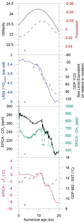
Figure 8 shows, for each interglacial, a range of key climate data sets. Each data set is plotted on its own age scale (i.e., there is no attempt at synchronizing), so spurious phasings may result. Each is presented with the same scales on each x and y axis, so that it is immediately possible to recognize long interglacials as opposed to short ones, and ones that are strong in a particular property. In each figure, the four panels relate to (Figure 8a) astronomical parameters (obli-quity and precession), (Figure 8b) indicators related to sea level (LR04 benthic oxygen isotope stack, and ODP1123 sea level esti-mate based on derived isotopic content of bottom water), (Figure 8c) GHG (CO2

and CH₄), and (Figure 8d) temperature (high-latitude North Atlantic SST (ODP982) and Antarctic air temperature (EPICA Dome C)).

6. The Intensity of Interglacials

Numerous records from the marine and terrestrial (including ice core) realm show a pattern in which the basic glacial-interglacial sequence is seen and in which peaks and troughs can easily be aligned (but not necessarily synchronized) with marine isotope stages (MIS) identified in marine benthic isotope records, such as the LR04 stack [Lisiecki and Raymo, 2005]. This indicates that, however, we define them, interglacial states are global phe-nomena, expressed in almost every type

Figure 8. Presentation of key data sets for each interglacial discussed in this paper. In each case after thisfirst expanded exemplar, the x axis (time) and y axis for each interglacial have approxi-mately the same scaling to allow comparison between interglacials. Each plot runs (right to left) from the preceding glacial period through the termination, across the interglacial peak, and into the inception of the following glacial period (except MIS 1 which stops at the present). (a) Obliquity and precession [Laskar et al., 2004]. (b) The LR04 benthic oxygen isotope stack [Lisiecki and Raymo, 2005], and the sea level estimate based on separating deepwater temperature and water isotopic content from a record at site ODP1123 (South Pacific) [Elderfield et al., 2012]. (c) The ice core record of CO2[Lüthi et al., 2008;

Bereiter et al., 2015] and CH4[Loulergue et al.,

2008]. (d) The temperature estimated fromδD at EPICA Dome C, Antarctica [Jouzel et al., 2007], and SSTs at the North Atlantic site ODP982 [Lawrence et al., 2009]. Thisfirst set of panels is for MIS 1.

of paleoenvironmental signal at every location. (Some tropical records are an exception to this: in particular, the Chinese speleothem record [Cheng et al., 2012] expresses strong precessional variability, but the interglacials (as we have defined them) do not stand out as unusual.) However, the intensity and precise timing of that expression varies between records and the different spatial and environmental patterns seen in each of them are important evidence to test against our understanding of the mechanisms behind them. In this section, we focus on the intensity or strength of interglacials.

In some cases we can relate the proxy record we use with a single climate parameter (for example, the ice core measurements of CO2or Mg/Ca in marine records representing

near surface temperature); in others (for example, the biosilica content of sediments in Lake Baikal) the association is more complex but still the glacial-interglacial pattern is seen. In each record one can define the intensity of the interglacial based on the extent to which the mea-sured parameter changes in the intergla-cial direction (higher CO₂, more arboreal pollen, less dust, etc.): this allows us to use a range of proxies without necessarily having a clear or unique interpretation of its meaning. In assessing the intensity of each interglacial, we therefore have a range of measures representing different aspects of the Earth sys-tem and different geographical regions.

A further issue to consider is whether one defines the intensity based on the maximum value achieved, or on the average over the entire interglacial or over a specified period. There are advantages and disadvantages to each approach:

1. Comparing the identical time period in each record would allow us to build the kind of snapshot climate reconstructions that are useful for comparison with most climate model outputs. However, the accuracy of the chronology in many records is variable, and our ability to synchronize records in any of the earlier interglacials is too low to allow such an approach in practice.

2. An average over the entire interglacial would probably be the most intuitive approach, allowing us to assess the integrated strength of an interglacial without assuming that the strength occurred simultaneously at every location. However, the period of averaging, and hence the result, is very dependent on the definitions used to determine the timing of the start and end of an interglacial, as discussed in section 7.5. In addition, this method carries an underlying assumption that there is a stable interglacial period over which it is possible to define stationary statistics, whereas in some parameters and interglacials no such period exists: rather, values approach a peak and immediately start to descend toward glacial values again.

3. Using the maximum value obtained during a particular interglacial puts focus on what may be a short anomalous period caused by local factors. This approach also suffers from the fact that we have records of varying resolution available, implying that we couldfind a maximum that is resolved in one record and miss it because it is unresolved in another. We must also be very aware that the maximum value may occur at different dates in different records, so that comparisons must not be used incorrectly. Nonetheless, it is very easy to define the maximum value objectively, it represents the value that