HAL Id: insu-01429786
https://hal-insu.archives-ouvertes.fr/insu-01429786
Submitted on 4 Aug 2020
HAL is a multi-disciplinary open access
archive for the deposit and dissemination of
sci-entific research documents, whether they are
pub-lished or not. The documents may come from
teaching and research institutions in France or
abroad, or from public or private research centers.
L’archive ouverte pluridisciplinaire HAL, est
destinée au dépôt et à la diffusion de documents
scientifiques de niveau recherche, publiés ou non,
émanant des établissements d’enseignement et de
recherche français ou étrangers, des laboratoires
publics ou privés.
according to the upstream solar wind electric field
Takuya Hara, Janet G. Luhmann, François Leblanc, Shannon M. Curry,
Kanako Seki, David A. Brain, Jasper S. Halekas, Yuki Harada, James P.
Mcfadden, Roberto Livi, et al.
To cite this version:
Takuya Hara, Janet G. Luhmann, François Leblanc, Shannon M. Curry, Kanako Seki, et al.. MAVEN
observations on a hemispheric asymmetry of precipitating ions toward the Martian upper atmosphere
according to the upstream solar wind electric field. Journal of Geophysical Research Space Physics,
American Geophysical Union/Wiley, 2017, 122 (1), pp.1083-1101. �10.1002/2016JA023348�.
�insu-01429786�
Journal of Geophysical Research: Space Physics
MAVEN observations on a hemispheric asymmetry
of precipitating ions toward the Martian upper
atmosphere according to the upstream
solar wind electric field
Takuya Hara1 , Janet G. Luhmann1 , François Leblanc2 , Shannon M. Curry1 ,
Kanako Seki3 , David A. Brain4 , Jasper S. Halekas5 , Yuki Harada1 , James P. McFadden1,
Roberto Livi1 , Gina A. DiBraccio6 , John E. P. Connerney6, and Bruce M. Jakosky4
1Space Sciences Laboratory, University of California, Berkeley, California, United States,2LATMOS/IPSL-CNRS, Université Pierre et Marie Curie, Paris, France,3Department of Earth and Planetary Science, Graduate School of Science, University of Tokyo, Tokyo, Japan,4Laboratory for Atmospheric and Space Physics, University of Colorado Boulder, Boulder, Colorado, United States,5Department of Physics and Astronomy, University of Iowa, Iowa City, Iowa, United States,6NASA Goddard Space Flight Center, Greenbelt, Maryland, United States
Abstract
The Mars Atmosphere and Volatile Evolution (MAVEN) observations show that the global spatial distribution of ions precipitating toward the Martian upper atmosphere has a highly asymmetric pattern relative to the upstream solar wind electric field. MAVEN observations indicate that precipitating planetary heavy ion fluxes measured in the downward solar wind electric field (−E) hemisphere are generally larger than those measured in the upward electric field (+E) hemisphere, as expected from modeling. The −E (+E) hemispheres are defined by the direction of solar wind electric field pointing toward (or away from) the planet. On the other hand, such an asymmetric precipitating pattern relative to the solar wind electric field is less clear around the terminator. Strong precipitating fluxes are sometimes found even in the +E field hemisphere under either strong upstream solar wind dynamic pressure or strong interplanetary magnetic field periods. The results imply that those intense precipitating ion fluxes are observed when the gyroradii of pickup ions are estimated to be relatively small compared with the planetary scale. Therefore, the upstream solar wind parameters are important factors in controlling the global spatial pattern and flux of ions precipitating into the Martian upper atmosphere.1. Introduction
The plasma environments around weakly magnetized planets, such as Mars and Venus, are highly variable depending on the upstream solar wind conditions, including the interplanetary magnetic field (IMF) strength and orientation. Planetary ions at Mars are energized from the direct interaction between the solar wind and the upper atmosphere, resulting in enough energy to escape to space [e.g., Dubinin et al., 2011; Lundin, 2011, and references therein]. In situ measurements, including those from Phobos 2, Mars Express (MEX), and recently the Mars Atmosphere and Volatile Evolution (MAVEN), have confirmed that planetary ions (O+, O+
2, and CO+2) are flowing outward from the planet [e.g., Lundin et al., 1989; Barabash et al., 2007; Jakosky et al., 2015a; Brain et al., 2015].
A number of ion energization and escape processes from Mars have been proposed [e.g., Chassefière and
Leblanc, 2004; Lillis et al., 2015, and references therein]. One of the most important processes for ions to acquire
energy is through the “pick up” process where planetary ions are picked up by the convecting IMF and accel-erated by the associated motional solar wind electric field. These pickup ions can be lost to space because gyroradii of picked up ions are generally larger than the planetary scale. On the other hand, a fraction of pickup ions may precipitate back into the Martian upper atmosphere [e.g., Leblanc et al., 2015]. Precipitating pickup ions play an important role in atmospheric escape, because they serve as a catalyst for sputtering, a process by which precipitating ions transfer their energy to the ambient neutral particles via cascade collisions. Consequently, some of these neutrals can acquire sufficient energy to overcome the Mars’ gravity and escape to space. Therefore, information on ion precipitation into the Martian upper atmosphere is important for understanding the atmospheric escape from Mars.
RESEARCH ARTICLE
10.1002/2016JA023348
Special Section:
Major Results From the MAVEN Mission to Mars
Key Points:
• MAVEN shows that the precipitating heavy ion fluxes are stronger in the −Ehemisphere rather than in the+E hemisphere
• Strong precipitating ion fluxes are detected even in the+Ehemisphere during the disturbed solar wind periods
• Gyroradii of pickup ions play an important role in controlling the precipitating ion patterns in MSE coordinates
Correspondence to: T. Hara,
Citation:
Hara, T., et al. (2017), MAVEN observations on a hemispheric asymmetry of precipitating ions toward the Martian upper atmo-sphere according to the upstream solar wind electric field, J. Geophys. Res. Space Physics, 122, 1083–1101, doi:10.1002/2016JA023348.
Received 25 AUG 2016 Accepted 4 JAN 2017
Accepted article online 7 JAN 2017 Published online 19 JAN 2017 Corrected 10 FEB 2017
This article was corrected on 10 FEB 2017. See the end of the full text for details.
©2017. American Geophysical Union. All Rights Reserved.
Numerous modeling studies have suggested that ion fluxes precipitating toward the Martian upper atmo-sphere do so in a highly asymmetric fashion according to the direction of the upstream solar wind electric field, defined by E = −V × B, where V is the solar wind velocity and B is the IMF direction [e.g., Luhmann and
Kozyra, 1991; Luhmann et al., 1992; Leblanc and Johnson, 2001, 2002; Fang et al., 2013; Wang et al., 2014, 2015; Curry et al., 2015]. Specifically, these results show that the precipitating planetary heavy ion fluxes in the −E
hemisphere are generally higher than those in the +E hemisphere [e.g., Luhmann and Kozyra, 1991; Chaufray
et al., 2007], while solar wind protons and picked up planetary protons are predicted to behave in an opposite
sense [e.g., Brecht, 1997; Kallio and Janhunen, 2001; Diéval et al., 2012a]. The −E (+E) hemispheres are defined as the halves of the Mars globe where the upstream solar wind electric field points toward (away from) the planet. Previous numerical simulations also suggested that sputtering loss for neutral particles from Mars is much smaller than the other atmospheric escape processes in the present epoch [e.g., Luhmann et al., 1992;
Chassefière and Leblanc, 2004; Chaufray et al., 2007]. However, in the early solar system (>3 Gyr ago), sputtering
could have been one of the dominant escape processes from Mars owing to the much stronger solar forcing from the solar wind and/or solar EUV flux [e.g., Luhmann et al., 1992]. Thus, understanding ion precipitation in the current Martian plasma environment is critical for extrapolating these losses back to earlier epoch. In situ measurements of precipitating ions began with Mars Express (MEX), which completed orbit insertion around Mars in late December 2003 [e.g., Chicarro et al., 2004; Barabash et al., 2006]. Hara et al. [2011] first reported that MEX observed enhancements of precipitating heavy ions, such as O+and O+
2, mostly coinciding with corotating interaction regions (CIRs) passages, suggesting that heavy ion precipitation (as well as any potential associated sputtering losses) is highly variable and depends on the upstream solar wind condi-tions at Mars. However, the absence of a magnetometer on board MEX prevented the direct investigation of the effects of the background convection electric field on ions precipitating toward the Martian upper atmosphere. Hara et al. [2013] attempted to address the dependence of the solar wind electric field on pre-cipitating heavy ions based on MEX observations by estimating the IMF orientation from the characteristics of velocity distribution functions of picked up exospheric protons around Mars, because they are generally gyrating in the plane perpendicular to the IMF direction [e.g., Yamauchi et al., 2006, 2008]. They confirmed that the locations where precipitating heavy ions were observed tend to be well organized along the inferred solar wind electric field direction [Hara et al., 2013].
Diéval et al. [2012b] first analyzed the behavior of precipitating protons on the Martian dayside ionosphere
using MEX plasma observations. They suggested that observations of precipitating protons are in good agree-ment with the characteristics of precipitating heavy ions [Hara et al., 2011]. In particular, Diéval et al. [2013a] statistically investigated precipitating protons observed by MEX, and demonstrated that precipitating proton fluxes are stronger in the +E hemisphere than in the −E hemisphere. In order to determine the direction of the solar wind electric field, however, they referred the IMF draping direction proxy derived from the Mars Global Surveyor (MGS) magnetic field measurements [Brain et al., 2006]. Since this proxy was obtained from the MGS measurements at an altitude of ∼400 km, in the magnetic pileup region below the bow shock, only broad trends, and not precise IMF directions can be derived from it. Diéval et al. [2013b] further investigated roles of the solar wind variations on precipitating protons in the Martian plasma environment. They reported that the occurrence frequency of precipitating proton events is reduced by a factor of ∼3 during the disturbed solar wind periods, indicating that the strong draped induced magnetosphere prevents protons from easily penetrating toward the Martian upper atmosphere owing to small proton gyroradii.
While there has been a significant amount of interest in ion precipitation at Mars, no study to date has inves-tigated the statistics of precipitating ions with in situ plasma and magnetic field measurements. The MAVEN spacecraft has been orbiting Mars since November 2014 [Jakosky et al., 2015b] with the objective of charac-terizing the structure and composition of the upper atmosphere/ionosphere and addressing physical pro-cesses driving atmospheric erosion. MAVEN’s elliptic orbit, designed to precess around Mars with a periapsis (apoapsis) altitude of ∼150 km (∼6200 km), enables its instruments to observe various plasma regimes includ-ing upstream solar wind, magnetosheath, induced magnetosphere, and ionosphere. MAVEN possesses the most comprehensive plasma instruments suite together with electric and magnetic field detectors, enabling us to more precisely diagnose the effects of the solar wind electric field on precipitating ion phenomena for the first time. Leblanc et al. [2015] studied an event where MAVEN observed precipitating O+ions during steady solar wind conditions. They suggested that precipitating ions are not intermittent but rather commonly detected in the Martian upper atmosphere. On the basis of the theoretical relationships between the observed total precipitating ion flux and expected sputtered escape flux [Wang et al., 2015], they proposed that neutral
Journal of Geophysical Research: Space Physics
10.1002/2016JA023348
atomic oxygen can be typically escaping due to sputtering at a rate as much as ∼1 × 1024s−1[Leblanc et al., 2015]. But sufficient data from MAVEN did not exist yet to perform a statistical analysis to determine the global behavior of pickup ions with respect to the convective electric field.
In order to understand the predicted electric field asymmetries, we must use the appropriate coordinate system. We refer to mainly two coordinate systems in this study: one is the Mars-centered Solar Orbital (MSO) coordinates, and the other is the Mars-centered Solar Electric field (MSE) coordinates. The MSO coordinate sys-tem is defined with the X axis toward the Sun, the Z axis perpendicular to the ecliptic pointing to the northern hemisphere, and the Y axis completing the right-hand system. Meanwhile, the MSE coordinate system is defined with the X axis toward the Sun, the Z axis along the upstream solar wind electric field, and the Y axis also completing the right-hand system. In this paper, we only use the MSE coordinate system for analysis. In this paper, we first present a global statistical map of ions precipitating toward the Martian upper atmo-sphere based on simultaneous MAVEN plasma and magnetic field observations, in order to observationally establish the existence of the hemispheric asymmetry controlled by the solar wind convection electric field. Section 2 describes the MAVEN data sets and instruments used in this study, and how to compute the ion fluxes precipitating toward the Martian upper atmosphere. Section 3 presents the examples of ion pre-cipitation in both the ±E hemispheres and the global statistical maps of precipitating ion fluxes in the MSE coordinates, obtained from the Solar Wind Ion Analyzer (SWIA) measurements [Halekas et al., 2015a]. Additionally, we present the dependence of the observed precipitating ion fluxes on energy and upstream solar wind conditions. Section 4 discusses comparable analyses of precipitating ions with the Suprathermal and Thermal Ion Composition (STATIC) analyzer [McFadden et al., 2015]. In section 5, we summarize our results and discuss crucial drivers that control the hemispheric asymmetry of precipitating ion fluxes toward the Martian upper atmosphere in MSE coordinates.
2. MAVEN Data Sets
In this work, we use two different ion instruments from MAVEN: the Solar Wind Ion Analyzer (SWIA) [Halekas
et al., 2015a, 2016] and the Suprathermal and Thermal Ion Composition (STATIC) analyzer [McFadden et al.,
2015]. SWIA is a cylindrically symmetric electrostatic analyzer with deflection optics, allowing the sampling of high-cadence ion velocity distributions with energies from ∼25 eV to ∼25 keV as fast as every 4 s with high-energy resolution (7.5%) and angular resolution (4.5∘ × 3.75∘ in the sunward direction, 22.5∘ × 22.5∘ elsewhere). The total field of view (FOV) is 360∘ × 90∘; SWIA cannot discriminate ion species [Halekas et al., 2015a, 2016]. STATIC adopts a similar toroidal electrostatic analyzer with a 360∘ × 90∘ FOV in combination with a time-of-flight (TOF) velocity analyzing system in order to discriminate ion species [McFadden et al., 2015]. STATIC is capable of operating over an energy range from ∼0.1 eV up to ∼30 keV also as fast as every 4 s with energy resolution (∼15%) and angular resolution (22.5∘ × 6∘). However, STATIC’s energy range dynami-cally changes according to the spacecraft altitude and/or attitude during every orbit. There are three primary energy sweep modes: Ram mode (0.1–50 eV) is typically used around periapsis (<200 km), Conic mode (0.1–500 eV) adjacent to periapsis (∼200–800 km), and Pickup mode (∼1–30,000 eV) is operated in the remaining higher-altitude range. Since STATIC is designed to characterize the behaviors of the Martian cold ionospheric ions at low altitude, it does not capture high-energy ion populations accelerated up to the ∼keV range in the vicinity of the Martian ionosphere. However, in additions to these three modes, STATIC can also operate in Protect mode (∼30–30,000 eV) to prevent damagingly high fluxes in case the spacecraft poten-tial goes sufficiently negative. This provides us with an opportunity to investigate the behavior of these high-energy ions in the Martian ionosphere. The higher dimensional data products including energy, angular, and mass arrays are only available every 16–128 s, depending on energy sweeping mode and the telemetry rate [McFadden et al., 2015]. The FOVs of SWIA and STATIC mostly overlap but are not completely identical, because they are mounted in different locations on the spacecraft. SWIA is mounted on the spacecraft main body and is designed to widely cover the Sun-nadir plane for most science operations. On the other hand, STATIC is mounted on the Articulated Payload Platform (APP) attached to a 2 m boom along with other instru-ments [McFadden et al., 2015]; therefore, STATIC’s FOV is highly variable depending on both the spacecraft and APP attitudes. MAVEN also has a triaxial fluxgate magnetometer (MAG) [Connerney et al., 2015], which is an essential instrument to investigate the dependence of the other measurements on the upstream solar wind electric field.
In this study, we computed the orbital average solar wind parameters based on the SWIA and MAG data, taking into account the spacecraft location. The time intervals during which MAVEN measured the upstream solar
wind outside of the Martian bow shock are automatically determined by the SWIA and MAG measurements (described in detail in Halekas et al. [2016]). For example, the upstream solar wind obtained from this method is used in Jakosky et al. [2015c]. Since the orbital period is approximately 4.5 h, it means upstream solar wind parameters derived from MAVEN observations at Mars are available about every 4.5 h, with the exception of orbits that are completely immersed in the sheath, never extending outside of the bow shock.
Precipitating ions are calculated under the assumption that any ions detected in either the SWIA or STATIC angular bins whose FOVs are within a cone angle of 75∘ along the positive radial direction relative to the center of Mars will precipitate into the Martian upper atmosphere. We only used data when the spacecraft was at an altitude between 200 and 350 km, as this altitude range is approximately close to the Martian exobase [e.g., Yagi et al., 2012] where precipitating ions are generally capable of colliding with ambient neutral par-ticles, resulting in sputtering loss of neutral particles [e.g., Luhmann and Kozyra, 1991; Luhmann et al., 1992;
Leblanc and Johnson, 2001, 2002]. The methodology used in this study is identical to that in Leblanc et al. [2015].
3. SWIA Observations of Precipitating Ions in the MSE Coordinates
3.1. Representative Events
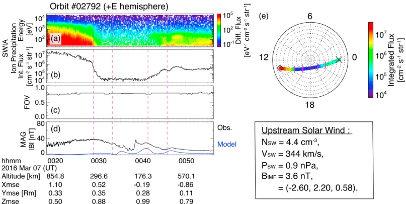
In this section, we present two representative events in which SWIA measured ions precipitating toward the Martian upper atmosphere in both the ±E hemispheres. Figures 1 (2) show overviews of the MAVEN mea-surements of precipitating ions below 1000 km in the +E (−E) hemispheres. Figures 1a and 2a are the SWIA energy-time spectrograms of precipitating ions, which are calculated by using SWIA data whose angular bins are directed within a cone angle of 75∘ relative to the local zenith direction, as described in section 2. Figures 1c and 2c are the FOV coverage, defined as the total solid angles summed over the SWIA angular bins used in calculations for precipitating ions, divided by the solid angle of a cone with apex angle 75∘, i.e., 2𝜋(1 − cos(75°)) ≃ 4.66 str.
There are several similar features seen between Figures 1 and 2:
1. SWIA continuously has a FOV coverage of ∼80% (∼3.73 str) to measure precipitating ions seen in Figures 1c and 2c.
2. Figures 1d and 2d suggest that the local magnetic field strength measured by MAG [Connerney et al., 2015] is moderate (≲60 nT), and the modeled crustal magnetic field from Morschhauser et al. [2014] is small. 3. The solar wind parameters are approximately similar between both orbits and common during the entire
MAVEN primary science phase (see section 3.2.3 for the detailed investigations of the solar wind depen-dences of precipitating ion fluxes). We listed the upstream solar wind parameters, including the number density (Nsw), velocity (Vsw), dynamic pressure (Psw), and the IMF (BIMF) strength and orientation in the MSO coordinates on the lower right corner of Figures 1 and 2.
4. Figures 1e and 2e indicate that MAVEN was traveling from dayside to nightside; however, they were in opposite E hemispheres.
The center of the displayed time interval corresponds to the MAVEN closest approach where the left and right halves of the time intervals show the MAVEN inbound and outbound crossings. There are two periods when MAVEN is located between 200 and 350 km (magenta dashed lines for the inbound and outbound legs). The overplotted magenta bars in Figures 1e and 2e correspond to the MAVEN locations for the times denoted by magenta dashed vertical lines in Figures 1a–1d and 2a–2d. The precipitating ion fluxes, integrated over the whole SWIA energy range (Figures 1b and 2b), are clearly shown to be stronger in the −E hemisphere rather than in the +E hemisphere, in particular, on the dayside. This patterns of precipitating ions seen in the MSE coordinates are consistent with previous numerical simulations [e.g., Luhmann and Kozyra, 1991; Chaufray
et al., 2007; Fang et al., 2013; Curry et al., 2015], under the assumption that heavy ions (i.e., heavier than helium)
are main constituents in the precipitating fluxes at this altitude range. In the following sections, we will present the statistical analyses of ions precipitating toward the Martian upper atmosphere based on the SWIA mea-surements at altitudes between 200 and 350 km in the MSE coordinates, such as in the time intervals between two pairs of magenta dashed vertical lines in Figures 1a–1d and 2a–2d or magenta bars in Figures 1e and 2e.
3.2. Statistical Global Ion Precipitation Patterns
To statistically investigate the global spatial pattern of ions precipitating toward the Martian ionosphere in the MSE coordinates, we surveyed time intervals from 1 December 2014 to 30 April 2016, when MAVEN can directly measure the solar wind. Owing to the MAVEN orbital configuration, there are three distinct blind
Journal of Geophysical Research: Space Physics
10.1002/2016JA023348
Figure 1. Overview of SWIA measurements of ions precipitating toward the Martian upper atmosphere at altitudes lower than 1000 km in the+Ehemisphere on 7 March 2016 (Orbit #2792): (a) the precipitating ion energy spectra observed by SWIA in units of differential number flux (“Diff. Flux”), (b) the integrated precipitating ion fluxes (“Int. Flux”) over the whole SWIA energy range, (c) the SWIA field of view (FOV) coverage for measuring precipitating ions, and (d) the local magnetic field strength for the MAVEN observations (“Obs.”; black) and the crustal field model (blue) [Morschhauser et al., 2014]. (e) The spacecraft trajectory is mapped on the basis of the Lambert azimuthal equal area projection in the+Ehemisphere and is color coded by the integrated precipitating ion fluxes (Figure 1b). The perimeter numbers describe the local time; the left half (right half ) of a map corresponds to the dayside (nightside), respectively. In this event, MAVEN was traveling from dayside (black diamond) to nightside (black cross). The orbital averaged upstream solar wind parameters, obtained from SWIA and MAG, are listed in the lower right corner.
periods when MAVEN could not make upstream solar wind observations outside the bow shock (mid-March 2015 to mid-June 2015, mid-October 2015 to early December 2015, and after mid-April 2016).
We used SWIA coarse survey data [Halekas et al., 2015a] to compute the ion flux precipitating toward the Martian ionosphere, excluding times when upstream solar wind data were not available. We singled out time periods when (1) the FOV of SWIA covers more than 70% of the 75∘ cone angle of the local zenith direction (see Figures 1c, and 2c); (2) in order to reduce an ambiguity of the coordinate transformation from MSO to MSE coordinates, we required that the standard deviation of the IMF clock angle,𝜓 ≡ arctan(By∕Bz), in the MSO coordinates within individual MAVEN orbits be smaller than 45∘, i.e.,|Δ𝜓| ≤ 45°, indicating that the IMF orientation is relatively stable. As a result of data filtering, 90,677 SWIA coarse survey 3-D distributions in total satisfied our selection criteria and were utilized in our statistical analyses. As mentioned in section 2, SWIA is unable to discriminate ion species [Halekas et al., 2015a]; however, we only focus on precipitating ions that are observed at altitudes of 200 to 350 km which is in the vicinity of the exobase [e.g., Yagi et al., 2012], where the planetary-origin heavy ions (such as O+, O+
2) are assumed to be the most dominant ion populations.
3.2.1. General Features
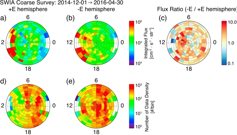
Figures 3a (3b) display the global statistical maps of precipitating ion fluxes integrated over the whole SWIA energy range for ions observed between 200 and 350 km over the +E (−E) hemispheres. The perimeter numbers shown in each map state the local time where the Sun is on the left. The energy-integrated total precipitating ion fluxes typically turn out to be the order of 104–106cm−2s−1str−1. Figure 3c is a statistical map of the precipitating ion flux ratio between ±E hemispheres, which is derived from Figure 3b normal-ized by Figure 3a. The blue-dominated areas in Figure 3c indicate that the precipitating ion fluxes observed in the −E hemisphere are weaker than those observed in the +E hemisphere, while the red-dominated areas indicate that the precipitating ion fluxes observed in the −E hemisphere are stronger than those observed in the +E hemisphere. Hence, these results indicate that the integrated precipitating ion fluxes differ in the
Figure 2. Overview of the SWIA measurements of precipitating ions below 1000 km in the−Ehemisphere on 15 September 2015 (Orbit #1874). The figure format is identical to Figure 1; however, Figure 2e is mapped on the basis of the Lambert azimuthal equal area projection in the−Ehemisphere.
dayside polar (around the latitude higher than 60∘ with the local time of 9–13 h) and nightside low-latitude region (around the latitude lower than 40∘ with the local time of 21–2 h) between the ±E hemispheres. In other words, the precipitating ion fluxes of the −E hemisphere are typically stronger than those of +E hemi-sphere in these regions. This observed hemispheric asymmetry of precipitating ions in the MSE coordinates, given our assumption of heavy ions dominating the precipitating fluxes, is consistent with previous numerical simulations [e.g., Luhmann and Kozyra, 1991; Chaufray et al., 2007; Fang et al., 2013; Curry et al., 2015]. On the other hand, the SWIA observations show that this hemispheric asymmetry of precipitating ions is rela-tively weak around the dawn-dusk terminator (4–8 h and 16–20 h). Interestingly, the precipitating ion fluxes in the +E hemisphere are slightly stronger than those in the −E hemisphere around the nightside polar region for the latitude higher than ∼50∘ with the local time of 21–3 h. While the strong precipitating ion fluxes are generally observed in the dayside subsolar region (≲40∘) in both the ±E hemispheres, the precipitating ion fluxes are typically stronger in the +E hemisphere rather than in the −E hemisphere (blue bins at low-latitude dayside in Figure 3c). These precipitating ion populations might be partially responsible for the penetrating double-charge exchange protons seen in the Martian upper atmosphere [Halekas et al., 2015b, 2016], rather than heavy ions; however, it has never been reported that these penetrating protons display an asymmetric distribution between the ±E hemispheres. A discussion of what ion species may be responsible for the hemi-spheric asymmetry of the ion precipitation in the MSE coordinates is left in section 4, where we investigate different precipitation maps for protons and heavy ions.
Figures 3d (3e) show the global distributions of the number of the SWIA 3-D measurements used in calculating precipitating ion fluxes in the +E (−E) hemispheres. Note that the data coverage on the nightside is better than that on the dayside in both the ±E hemispheres. Note also that there is no data coverage around the subsolar and antisubsolar regions, because MAVEN has never explored these regions in the altitude range of 200–350 km nor did MAVEN directly measure the solar wind due to the orbital configuration, preventing us from converting those results to MSE coordinates.
3.2.2. Energy Dependence
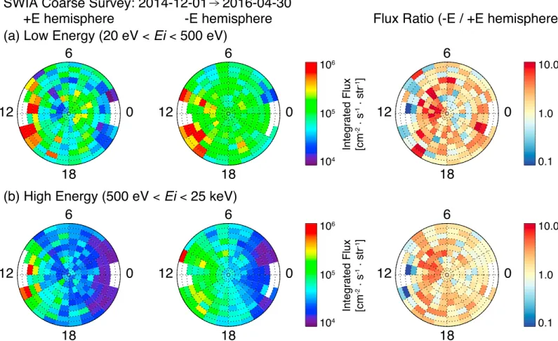
We separated Figure 3 into two different SWIA energy ranges; 20 eV< Ei< 500 eV, and 500 eV < Ei< 25 keV, in order to understand the energy dependence of ion precipitation. In the low-energy plots (Figure 4a), the basic ion precipitation patterns are similar to Figure 3, although the hemispheric asymmetry relative to the
Journal of Geophysical Research: Space Physics
10.1002/2016JA023348
Figure 3. Statistical global map of precipitating ions in both the (a)+Eand (b)−Ehemispheres at altitudes from 200 to 350 km, observed by SWIA from 1 December 2014 to 30 April 2016. These statistical maps are color contoured according to the precipitating ion fluxes integrated over the whole SWIA energy range. The total precipitating ion fluxes are averaged over this altitude range and binned as a function of longitude and latitude in MSE coordinates by 15∘ (=1 h local time)×10∘. The bins are mapped on the basis of the Lambert azimuthal equal area projection. The mapped binning resolutions are reduced for visualization around the polar area. The perimeter numbers describe the local time with the Sun to the left. (c) A flux ratio map of precipitating ions in the−E
hemisphere to those in the+Ehemisphere. Figure 3c is obtained from Figure 3b normalized by Figure 3a. Figures 3d (3e) are in the same formats as Figures 3a (3b) for the+E(−E) hemispheres; they are color contoured by the total number of SWIA 3-D distributions used in the statistical analyses.
upstream motional electric field is more obvious than in Figure 3. Meanwhile, the precipitation maps of high-energy ions (Figure 4b) show a clear day-night asymmetry with precipitating ion fluxes sharply decreas-ing on the nightside in the local time sector between ∼20 and 4 h in the −E hemisphere. In contrast, significant precipitating ion fluxes are only measured on the dayside in the local time from ∼9 to 17 h in the +E hemisphere. It should be noted that the precipitating ion flux levels observed in the nightside region are comparable between the ±E hemispheres.
3.2.3. Solar Wind Dependence
In this section, we further investigate the dependence of precipitating ions on the solar wind in MSE coor-dinates, using the same display format as in Figure 3 but with the specified upstream solar wind conditions. Figure 5 represents differences in the ion precipitation maps during periods of weak and strong solar wind dynamic pressure (Psw), where weak and strong are defined as Psw< 1 nPa and Psw> 1 nPa because the aver-age Pswis ∼0.94 with a standard deviation of 0.85 nPa during the whole surveyed interval. During the strong
Pswperiods in Figure 5b, a hemispheric asymmetry of precipitating ion fluxes is more obvious, and the inte-grated precipitating ion fluxes are typically enhanced approximately by an order of magnitude, especially on the dayside −E hemisphere. The blue-dominated areas in the flux ratio map near the nightside polar region for MSE latitudes higher than ∼60∘ indicate that MAVEN measured intense precipitating ion fluxes even in the +E hemisphere under the strong Pswconditions. Figure 6 similarly displays the ion precipitation maps under weak and strong IMF strength|B| periods, where weak and strong are defined as |B| < 4 nT and |B| > 4 nT, because the average|B| is ∼3.73 with a standard deviation of 2.12 nT during the whole surveyed interval. The global precipitation patterns tend to be similar to Figure 5; namely, intense precipitating ion fluxes are sporad-ically observed in the nightside polar region in the +E hemisphere during the strong IMF periods (Figure 6b).
Figure 4. Statistical averaged maps of precipitating ion fluxes integrated over the SWIA (a) low (20 eV< Ei< 500eV) and (b) high (500 eV< Ei< 25keV) energy range, observed at altitudes between 200 and 350 km from 1 December 2014 to 30 April 2016 in the (left column)+Eand (middle column)−Ehemispheres, whereEimeans the ion energy. The figure format is the same as in Figures 3a–3c.
It should be noticed that the representative events shown in section 3.1 (Figures 1 and 2) were thus observed under nominal solar wind conditions.
Here we investigate the effects of the gyroradii of pickup ions on the global ion precipitation maps in the MSE coordinates, taking into account the upstream solar wind velocity and IMF orientations. We assumed that the pickup ions are O+; therefore, the gyroradii of pickup O+ions are computed to be R
g= m|V⟂|∕qBsw, where
mis the oxygen ion mass, V⟂is ion velocity perpendicular to the IMF, Bswis the upstream IMF strength, and
qis the electric charge. This perpendicular ion velocity V⟂is also inferred from the upstream solar wind data. For example, the gyroradii of pickup O+ions can be calculated to be ∼2.2 × 10⁴km, in this case the solar wind is assumed to be flowing at a velocity of 400 km/s perpendicular to the IMF with a strength of 3 nT. Indeed, the gyroradii of pickup O+ions have a mean and standard deviation of 2.34 × 10⁴± 1.48 × 10⁴km during the whole surveyed interval. Figures 7a (7b) show ion precipitation maps under the time intervals when the gyroradii of pickup O+ions are estimated to be small (large), i.e., R
g< 20, 000 km (Rg>20, 000 km). Indeed, a hemispheric asymmetry of precipitating ion fluxes is more obvious when the gyroradii of pickup O+ions are relatively small (Figure 7a). Strong precipitating ion fluxes are also observed in the nightside polar region in the +E hemisphere, i.e., the blue-dominated areas in the right column of Figure 7a, suggesting that the gyroradii of pickup ions determined by the upstream solar wind conditions are one of the most important factors in controlling the ion precipitation maps in the MSE coordinates. Although strong precipitating ion fluxes are always detected regardless of the upstream solar wind conditions in the dayside low-MSE latitude region (≲40∘) in both ±E hemispheres, precipitating ion fluxes are stronger in the +E hemisphere rather than in the −E hemisphere. On the other hand, such a hemispheric asymmetry is relatively faint in the nightside under the large gyroradii periods (Figure 7b). Therefore, the “conventional” hemispheric asymmetry of precipitating ions, that the precipitating ion fluxes of the −E hemisphere are typically stronger than those of +E hemisphere,
Journal of Geophysical Research: Space Physics
10.1002/2016JA023348
Figure 5. Statistical averaged maps of precipitating ion fluxes integrated over the whole SWIA energy range in both the (left column)+Eand (middle column)
−Ehemispheres. The fluxes are averaged over altitudes between 200 and 350 km, observed by SWIA under the (a) weak (<1 nPa) and (b) strong (>1 nPa) solar wind dynamic pressure (Psw) periods from 1 December 2014 to 30 April 2016. The figure format is the same as in Figure 3.
Figure 6. Statistical averaged maps of precipitating ion fluxes integrated over the whole SWIA energy range in both the (left column)+Eand (middle column)
−Ehemispheres. The fluxes are averaged over altitudes between 200 and 350 km, observed by SWIA under the (a) weak (<4 nT) and (b) strong (>4 nT) IMF strength (|B|) periods from 1 December 2014 to 30 April 2016. The figure format is completely identical to Figure 5.
Journal of Geophysical Research: Space Physics
10.1002/2016JA023348
Figure 7. Statistical averaged maps of precipitating ion fluxes integrated over the whole SWIA energy range in both the+E(left column) and−E(center column) hemispheres. The fluxes are averaged over altitudes between 200 and 350 km, observed by SWIA under the (a) small (<20000 km) and (b) large (>20000 km) gyroradii (Rg) periods for O+from 1 December 2014 until 30 April 2016. This gyroradii are equivalent to∼5.9 Martian radii (Rm). The figure format is completely
Figure 8. (top row) The spectra of median values of precipitating ion fluxes with standard errors and (bottom row) the histograms of the number of the SWIA
data (bold black lines, leftyaxis) as a function of the (left) upstream solar wind dynamic pressure, the (middle) IMF strength, and the (right) estimated gyroradius of O+ions in the dayside+E(red), the dayside−E(blue), the nightside+E(magenta), and the nightside−E(black) hemisphere, respectively. The background
stacked percentage bar charts in the bottom row show the relative observation frequency of each area (rightyaxis). The SWIA data is collected to the largest values bin, when the upstream solar wind dynamic pressure is larger than 4 nPa, the IMF strength is larger than 11 nT, and the estimated gyroradius of O+ions
is larger than 15Rm, whereRmmeans the Martian radii (≃ 3389.9km).
is only seen in limited areas, such as in the dayside polar region with MSE latitudes higher than ∼40∘, or in the deep nightside with MSE latitudes lower than ∼40∘ during the small gyroradii periods.
Here we further investigate the behavior of precipitating ion fluxes as a function of upstream solar wind parameters, by dividing these global statistical maps in the MSE coordinates into four major areas, according to the ±E hemispheres and dayside/nightside. Figure 8 summarizes the median spectra of the precipitating ion fluxes (top row) and the total number of the SWIA measurements (bottom row) as a function of the upstream solar wind dynamic pressure (left column), the IMF strength (middle column), and the estimated gyroradius of O+ions (right column), observed in the dayside +E (red), the dayside −E (blue), the night-side +E (magenta), and the nightnight-side −E (black) hemispheres. Figure 8 shows interesting results for the solar wind dependences of precipitating ion fluxes described above. In particular, the integrated precipitating ion fluxes significantly increase as the upstream solar wind dynamic pressure also increases, and the precipitat-ing ion fluxes observed in the −E hemisphere are typically stronger than those in the +E hemisphere. But the precipitating ion fluxes appear to be approximately comparable between the ±E hemispheres when the IMF was strong or the estimated gyroradii of O+ions were large, which could be interpreted as an effect of finite gyroradii. Note that the large spike in precipitating ion fluxes were recorded for the second highest Psw bin. We confirmed that they are mostly coincident with the high solar wind density periods associated with the CIR passages just ahead of the stream interface. During these periods, the observed locations were mostly concentrated around the terminator in both the ±E hemispheres.
Journal of Geophysical Research: Space Physics
10.1002/2016JA023348
However, it should be mentioned here that the precipitating ion fluxes have a large difference in the dayside and nightside regions for each E hemisphere. For example, the precipitating ion fluxes vary by at least an order of magnitude with the MSE latitude in the dayside +E hemisphere (see, the left-half area of Figure 3a). This indicates that Figure 8 is currently insufficient in statistics, because the SWIA data coverage is not uniform in the MSE coordinates among the binned solar wind conditions (i.e., each bin in Figure 8). Therefore, Figure 8 must be statistically verified in the future on the basis of the larger data set.
4. Comparable Analyses Based on the STATIC Observations
We next performed analyses comparable to the SWIA results shown in section 3 based on the STATIC obser-vations. STATIC produces 22 different data products in total, and we first used the STATIC “CA” data product, whose measurement arrays are 16E × 4D × 16A, where E = energy, D = deflection, and A = azimuth anode. The STATIC CA data products have no ion mass (M) information; however, they are available as fast as every 4 s [McFadden et al., 2015]. Hence, their data structures are rather close to those of SWIA, allowing us to directly compare the precipitating ion maps in the MSE coordinates between SWIA and STATIC as a first step. It should be noted that STATIC mostly operates in Conic mode (∼0.1–500 eV) at altitudes between 200 and 350 km, on which we focused to compute precipitating ion fluxes, because STATIC is nominally designed to investigate the Martian ionospheric cold ions as mentioned in section 2. For the sake of comparable inves-tigations between SWIA and STATIC, we only considered precipitating ions with energies higher than 20 eV. Moreover, we also used the data when STATIC operates in Protect mode (∼30 eV–30 keV), which has similar energy coverage to SWIA.
There are a couple of specific caveats in order to calculate precipitating ion fluxes from STATIC. As mentioned in section 2, STATIC is mounted on the APP boom [McFadden et al., 2015]; therefore, the STATIC FOV is highly variable depending on both the spacecraft and APP attitudes. We took into account blockage of the STATIC FOV by the spacecraft by excluding the STATIC angular bins that are blocked by 50% or more in this study. Since STATIC data include 16 different quality flags that indicate the data quality [McFadden et al., 2015], we also excluded bad quality flags data in this study. With this data filtering, along with the same selection criteria used for SWIA discussed in section 3, 51,938 (25,143) STATIC CA 3-D distributions were obtained during the Conic (Protect) modes, which we used to generate the STATIC precipitating ion maps in MSE coordinates. Figure 9 illustrates the statistical ion precipitation maps in MSE coordinates obtained from the STATIC CA data product. STATIC also measured a hemispheric asymmetry in the precipitating ion fluxes relative to the upstream motional solar wind electric field. In other words, the precipitating ion fluxes detected in the −E hemisphere are generally stronger than those detected in the +E hemisphere. Note that this result is con-sistent with our assumption that heavy ions dominate the precipitating fluxes. This tendency is similarly consistent with previous numerical simulations [e.g., Luhmann and Kozyra, 1991; Chaufray et al., 2007; Fang
et al., 2013; Curry et al., 2015]. When STATIC is in the Conic mode (Figure 9a), the global ion precipitation
patterns resemble the SWIA result at low energy (Figure 4a), given that the energy range is similar between the two figures. On the other hand, Figure 9b appears to show somewhat different ion precipitation patterns when STATIC is in the Protect mode. The main reason may be that the STATIC FOV during the Protect mode differs from the FOV in the usual spacecraft attitude. Especially on the nightside, the spacecraft attitude when STATIC used the Protect mode may not have been suitable to measure the precipitating ions, causing the data coverage to be insufficient on the nightside of Figure 9 regardless of the ±E hemispheres.
The STATIC 4-D data arrays including energy, deflection, azimuth anode, and mass are the most suitable to understand the behaviors of precipitating ions for each species. However, the time resolution of these data products is 32 or 4 s for the Conic mode, and 128 or 16 s for the Protect mode whether the data types are “Survey” or “Archive” (=“Burst”)[see McFadden et al., 2015], where MAVEN operates in the altitudes between 200 and 350 km. In terms of the Protect mode, only 4255 STATIC 3-D measurements with mass information are obtained using our selection criteria from 1 December 2014 to 30 April 2016, where we use both the STATIC “D0” and “D1” data products (32E × 4D × 16A × 8M). The amount of available data indicates that it is premature to conduct statistical investigations using these data products, because there are ∼5 times fewer measurements than those used in the results in Figure 9b.
In contrast, the STATIC 4-D survey (archive) data product was initially “CE” (“CF”) for the Conic mode, whose measurement arrays are 16E × 4D × 16A × 16M. However, the STATIC CE (CF) products were no longer supplied
Figure 9. Statistical averaged maps of precipitating ion fluxes integrated over the energy range (a) between 20 and 500 eV, and (b) between∼30 eV and 30 keV in both the (left column)+Eand (middle column)−Ehemispheres. These fluxes are averaged over altitudes between 200 and 350 km, obtained from the STATIC CA data products when STATIC operated (a) Conic and (b) Protect modes from 1 December 2014 to 30 April 2016. The figure format is basically identical to the SWIA maps (e.g., Figure 3).
Journal of Geophysical Research: Space Physics
10.1002/2016JA023348
Figure 10. Statistical averaged maps of the proton to heavy ions ratio of precipitating ion fluxes integrated over the
energy range (a) between 20 and 500 eV, and (b) between∼30 eV and 30 keV toward the Martian upper atmosphere in both (left column)+Eand (right column)−Ehemispheres. The fluxes are averaged over altitudes between 200 and 350 km, obtained from the STATIC CA and C6 data products when STATIC operated (a) Conic and (b) Protect modes from 1 December 2014 to 30 April 2016.
after July 2015 and are currently combined into D0 (D1) instead. Thus, it is similarly not straightforward to analyze the STATIC 4-D data during the Conic mode because the measurement arrays are different.
Taking into account the analysis restrictions for the STATIC 4-D data mentioned above, here we propose the current best approach to address the behaviors of precipitating ions for both protons and heavy ions: STATIC also continuously provides several other data products that sum over angular bins but the time resolution is as high as every 4 s. The STATIC “C6” data product, whose measurement arrays are 32E × 64M, is always available with a cadence of every 4 s. These time steps of the C6 data product are completely identical to those of the CA data product. Therefore, we first computed the count rate ratio of protons and heavy ions relative to all ions at each STATIC energy step from the C6 data. After that, we were able to estimate global maps of precipitating ion fluxes in the MSE coordinates for both the protons and heavies by multiplying these ion count ratios by the CA data product as utilized in Figure 9, under the assumption that this ion count rate ratio is uniform regardless of the STATIC angular bins.
Figure 10 shows global maps of the total precipitating ion flux ratio between protons and heavy ions in the MSE coordinates, obtained from the STATIC CA and C6 data products. The blue-dominated areas indicate that
precipitating heavy ions are more dominant than protons, while the red-dominated areas indicate that pre-cipitating protons are more dominant than heavies. It is clearly shown that heavy ions are most of the time the major species precipitating at altitudes between 200 and 350 km, which confirms that our assumption of heavy ion dominance is correct. In Conic mode (Figure 10a), precipitating protons are the more dominant populations rather than precipitating heavy ions in several areas, especially in the dayside terminator in the +E hemisphere and to some extent in −E hemisphere. In Protect mode (Figure 10b), such a tendency also appears to be intermittently seen in the +E hemisphere. MAVEN observations thus suggest that pickup pro-tons originating in the exosphere [e.g., Barabash et al., 1991; Dubinin et al., 2006; Yamauchi et al., 2006] and/or shocked solar wind protons [e.g., Brecht, 1997; Kallio and Janhunen, 2001; Diéval et al., 2012a] tend to favor precipitating toward the dayside in the +E hemisphere. Jarvinen et al. [2010, 2013, 2016] suggest that the proton gyroradii are much smaller than those of heavy ions such that their motion follows more closely the
E × B drift than for heavy ions, based on the results from their hybrid simulations. Their hybrid simulations
also show that the E × B drifting streamlines in the +E hemisphere are mostly pointing to the planet, while their streamlines in the −E hemisphere lead to the planetary wake. This result indicates that protons born in the +E hemisphere can more easily precipitate toward the planet rather than those born in the −E hemi-sphere [Jarvinen et al., 2010, 2013, 2016]. Therefore, our results associated with the hemispheric asymmetry of precipitating protons in the MSE coordinates are in good agreement with their hybrid simulations prediction [Jarvinen et al., 2010, 2013, 2016].
On the other hand, we pointed out a potential possibility that penetrating protons [Halekas et al., 2015b, 2016] could play a role in controlling a hemispheric asymmetry of precipitating ions in the dayside low-MSE lati-tude region in section 3.2.1. However, it is somewhat difficult to determine which protons or heavy ions are dominant precipitating populations in the dayside low-MSE latitude region because sufficient data coverage is lacking in Figure 10. It should be noticed that we tested creating similar figures to Figure 10 by simply using different STATIC data products, such as D0 and D1 (32E × 4D × 16A × 8M) or D4 (4D × 16A × 2M) [McFadden
et al., 2015], even though the data volumes seem to be statistically insufficient. We verified that the resultant
precipitating flux ratio maps between protons and heavy ions tend to be similar to Figure 10 (not shown here).
5. Summary and Discussions
In this paper, we statistically investigate patterns of ion precipitation into the Martian atmosphere at altitudes between 200 and 350 km in MSE coordinates, based on measurements from both the SWIA and STATIC instru-ments on MAVEN. This analysis was made possible by the availability of MAVEN magnetometer data, allowing the determination of the upstream magnetic fields. The SWIA observations demonstrated that the integrated precipitating ion fluxes are globally stronger in the −E hemisphere than in the +E hemisphere, which is con-sistent with the assumption that the precipitating ion flux is dominated by heavy ions. The energy-integrated total precipitating ion fluxes are typically of the order between 104and 106cm−2s−1str−1. This hemispheric asymmetry of precipitating ion fluxes with respect to the solar wind electric field is consistent with previous numerical predictions [e.g., Luhmann and Kozyra, 1991; Chaufray et al., 2007; Fang et al., 2013; Curry et al., 2015]. Strong precipitating ion fluxes are detected around the dayside lower MSE latitudes regardless of the ±E hemispheres, which is also in good agreement with previous numerical simulations [Chaufray et al., 2007]. In particular, precipitating ions with energies larger than 500 eV are frequently measured on the dayside rather than on the nightside (Figure 4b).
Comparing disturbed solar wind periods with quiet periods, precipitating ion fluxes are statistically enhanced by at least an order of magnitude during disturbed solar wind periods (Figures 5 and 6). Hara et al. [2011] noticed that precipitating heavy ions are not always observed by MEX but are often associated with CIR passages. However, they only focused on the events in which significant precipitating ion fluxes sufficiently larger than the MEX instrument noise level were recorded. This suggests that MEX detected strong precipitat-ing heavy ions mostly coincident with CIR passages. The current results derived from the MAVEN observations are thus consistent with the previous MEX results [Hara et al., 2011].
On the other hand, intense precipitating ion fluxes are occasionally observed even in the +E hemisphere rather in the −E hemisphere, when the gyroradii of picked up O+ions are estimated to be relatively small (Figure 7a). This result suggests that the gyroradii of picked up ions, determined by the upstream solar wind properties, can play a significant role in determining the global patterns of ions precipitating toward the Martian upper atmosphere in the MSE coordinates. This interpretation is schematically illustrated in Figure 11.
Journal of Geophysical Research: Space Physics
10.1002/2016JA023348
Figure 11. Schematic illustrations of precipitating picked up ions trajectories under (a) large and (b) small gyroradii
periods. The directions of the solar wind flow and electromagnetic (EandB) fields are indicated by the black solid arrows on the left side. The background gradation colored as orange indicates the Martian exosphere. The white circles with numbers are representative picked up ions and their trajectories are shown as black curved arrows. The dotted circles are the approximate altitudes for which we adopted to calculate precipitating ion fluxes.
Under the large gyroradii periods in Figure 11a, pickup ions generated in the −E hemisphere can be acceler-ated sufficiently up to the high-energy regime and precipitate to the dayside low-MSE latitude (label 1), and to the −E hemisphere (labels 2 and 3). However, the ions precipitating toward the nightside −E hemisphere (label 3) do not substantially contribute to the precipitating ion fluxes because they are moving tailward (we regard ion populations moving radially inward toward the planet as precipitating ions). On the other hand, it is difficult for pickup ions born on both the dayside lower MSE latitude region and the +E hemisphere (label 4) to precipitate toward the Martian upper atmosphere because of their larger gyroradii compared to the planetary scale. Compared with the high-altitude region, where test particles labeled as 1–4 in Figure 11a are picked up, the ion densities are generally larger and the gyroradii of pickup ions are somewhat smaller in the relatively low-altitude region (such as the Martian magnetosheath and induced magnetosphere), because the flow speed is slower due to the mass loading, and the magnetic field is piled up around the planet. Hence, a portion of the initial gyration phase of the pickup ions has not sufficiently accelerated yet, but they result in precipitation in the −E hemisphere (label 5). On the other hand in the +E hemisphere, some final gyration phase of pickup ions that are in the low-energy regime could be seen in the +E hemisphere (label 6). During the small gyroradii periods in Figure 11b, high-energy accelerated pickup ions can precipitate not only in the −E hemisphere (labels 1 and 2) but also in the +E hemisphere (label 4; see, Figure 7a), because the gyroradii of pickup ions are approximately comparable to the planetary scale. The test particles (label 3) born on the nightside −E hemisphere can no longer precipitate, resulting in moving tailward into presumably interplanetary space. In the relatively low-altitude region, some low-energy pickup ion populations under the initial gyration phase born in the −E hemisphere (label 5) or the final gyration phase born in the +E hemisphere (label 6) could be measured in both hemispheres.
In the +E hemisphere, while some precipitating ion fluxes are detected on the nightside, their fluxes tend to be relatively weak on the dayside. Jarvinen et al. [2013, 2016] pointed out that the magnetic barrier is stronger on the +E hemisphere than on the −E hemisphere on the dayside, indicating that it can prevent pickup ions from more effectively precipitating in the +E hemisphere rather than in the −E hemisphere by deflecting them. Indeed, Masunaga et al. [2016] reported that some pickup ions precipitating toward the Martian upper atmosphere are reflected back to the solar wind based on MAVEN observations.
As the STATIC instrument on MAVEN allows the ion composition to be determined, we obtained similar ion precipitation maps in order to compare the SWIA and STATIC results, shown in Figures 3 and 9. According to the current STATIC data sets, Figure 10 suggested that the main species precipitating toward the Martian upper atmosphere are likely heavy ions; however, precipitating protons fluxes might be stronger than heavy ions around the dayside +E hemisphere because of finite gyroradii effects. This result is still subject to further investigation because we have not yet obtained large amounts of STATIC 4-D (e.g., D0 and D1) data products
sufficient to perform the statistical analyses. Therefore, this possibility needs to be verified from a larger 4-D STATIC database in the future.
Mars is known to possess highly asymmetric crustal magnetic fields primarily localized in the southern hemi-sphere [e.g., Acuña et al., 1998, 1999]. Hence, these crustal magnetic topologies around Mars are also capable of modulating the behaviors of ions precipitating toward the Martian upper atmosphere. Li et al. [2011] inves-tigated the effects of the crustal field on precipitating O+ ions toward the Martian upper atmosphere by using test particle simulations. They suggested that the crustal field can increase the O+ ion precipitation substantially, allowing the sputtering to be enhanced by a factor of ∼2 [Li et al., 2011]. Wang et al. [2015] found that the crustal fields can only modulate the O+ion precipitation rates within a factor of 2, while the upstream solar wind conditions allow O+ion precipitation rates to vary by a factor of more than 2 at least [Wang et al., 2014]. Wang et al. [2014] also suggested that the resultant sputtering escape rate can be enhanced by a factor of ∼50 depending on the upstream solar wind conditions. Indeed, Figures 5 and 6 also confirm that precipitating ion fluxes can be enhanced at least by an order of magnitude during disturbed solar wind periods. Therefore, the solar wind is the most significant factor in controlling the behavior of precipitating ions into the Martian upper atmosphere, while the crustal magnetic field topologies could be a secondary contributor. Future investigations are necessary to quantitatively understand the effects of the crustal mag-netic fields on the ions precipitating toward the Martian upper atmosphere, by using larger data sets of the still-accumulating MAVEN observations.
References
Acuña, M. H., et al. (1998), Magnetic field and plasma observations at Mars: Initial results of the Mars Global Surveyor mission, Science, 279, 1676–1680, doi:10.1126/science.279.5357.1676.
Acuña, M. H., et al. (1999), Global distribution of crustal magnetization discovered by the Mars Global Surveyor MAG/ER Experiment, Science, 284, 790–793, doi:10.1126/science.284.5415.790.
Barabash, S., A. Fedorov, R. Lundin, and J.-A. Sauvaud (2007), Martian atmospheric erosion rates, Science, 315, 501–503, doi:10.1126/science.1134358.
Barabash, S., E. Dubinin, N. Pisarenko, R. Lundin, and C. T. Russell (1991), Picked-up protons near Mars: Phobos observations, Gephys. Res. Lett., 18, 1805–1808, doi:10.1029/91GL02082.
Barabash, S., et al. (2006), The analyzer of space plasmas and energetic atoms (ASPERA-3) for the Mars Express mission, Space Sci. Rev., 126, 113–164, doi:10.1007/s11214-006-9124-8.
Brain, D. A., D. L. Mitchell, and J. S. Halekas (2006), The magnetic field draping direction at Mars from April 1999 through August 2004, Icarus, 182, 464–473, doi:10.1016/j.icarus.2005.09.023.
Brain, D. A., et al. (2015), The spatial distribution of planetary ion fluxes near Mars observed by MAVEN, Geophys. Res. Lett., 42, 9142–9148, doi:10.1002/2015GL065293.
Brecht, S. H. (1997), Solar wind proton deposition into the Martian atmosphere, J. Geophys. Res., 102, 11,287–11,294, doi:10.1029/97JA00561.
Chassefière, E., and F. Leblanc (2004), Mars atmospheric escape and evolution; interaction with the solar wind, Planet. Space Sci., 52, 1039–1058, doi:10.1016/j.pss.2004.07.002.
Chaufray, J. Y., R. Modolo, F. Leblanc, G. Chanteur, R. E. Johnson, and J. G. Luhmann (2007), Mars solar wind interaction: Formation of the Martian corona and atmospheric loss to space, J. Geophys. Res., 112, E09009, doi:10.1029/2007JE002915.
Chicarro, A., P. Martin, and R. Trautner (2004), The Mars Express mission: An overview, in Mars Express: A European Mission to the Red Planet, Eur. Space Agency Spec. Publ., ESA SP-1240, edited by A. Wilson and A. Chicarro, pp. 3–16, ESA Publ. Div., ESTEC, Noordwijk, Netherlands. Connerney, J. E. P., J. Espley, P. Lawton, S. Murphy, J. Odom, R. Oliversen, and D. Sheppard (2015), The MAVEN magnetic field investigation,
Space Sci. Rev., 195, 257–291, doi:10.1007/s11214-015-0169-4.
Curry, S. M., J. Luhmann, Y. Ma, M. Liemohn, C. Dong, and T. Hara (2015), Comparative pick-up ion distributions at Mars and Venus: Consequences for atmospheric deposition and escape, Planet Space Sci., 115, 35–47, doi:10.1016/j.pss.2015.03.026.
Diéval, C., E. Kallio, G. Stenberg, S. Barabash, and R. Jarvinen (2012a), Hybrid simulations of proton precipitation patterns onto the upper atmosphere of Mars, Earth Planets Space, 64, 121–134, doi:10.5047/eps.2011.08.015.
Diéval, C., et al. (2012b), A case study of proton precipitation at Mars: Mars Express observations and hybrid simulations, J. Geophys. Res., 117, A06222, doi:10.1029/2012JA017537.
Diéval, C., G. Stenberg, H. Nilsson, and S. Barabash (2013a), A statistical study of proton precipitation onto the Martian upper atmosphere: Mars Express observations, J. Geophys. Res. Space Physics, 118, 1972–1983, doi:10.1002/jgra.50229.
Diéval, C., G. Stenberg, H. Nilsson, N. J. T. Edberg, and S. Barabash (2013b), Reduced proton and alpha particle precipitations at Mars during solar wind pressure pulses: Mars Express results, J. Geophys. Res. Space Physics, 118, 3421–3429, doi:10.1002/jgra.50375.
Dubinin, E., M. Fränz, J. Woch, S. Barabash, R. Lundin, and M. Yamauchi (2006), Hydrogen exosphere at Mars: Pickup protons and their acceleration at the bow shock, Geophys. Res. Lett., 33, L22103, doi:10.1029/2006GL027799.
Dubinin, E., M. Fraenz, A. Fedorov, R. Lundin, N. Edberg, F. Duru, and O. Vaisberg (2011), Ion energization and escape on Mars and Venus, Space Sci. Rev., 162, 173–211, doi:10.1007/s11214-011-9831-7.
Fang, X., S. W. Bougher, R. E. Johnson, J. G. Luhmann, Y. Ma, Y.-C. Wang, and M. W. Liemohn (2013), The importance of pickup oxygen ion precipitation to the Mars upper atmosphere under extreme solar wind conditions, Geophys. Res. Lett., 40, 1922–1927, doi:10.1002/grl.50415.
Halekas, J. S., E. R. Taylor, G. Dalton, G. Johnson, D. W. Curtis, J. P. McFadden, D. L. Mitchell, R. P. Lin, and B. M. Jakosky (2015a), The solar wind ion analyzer for MAVEN, Space Sci. Rev., 195, 125–151, doi:10.1007/s11214-013-0029-z.
Halekas, J. S., et al. (2015b), MAVEN observations of solar wind hydrogen deposition in the atmosphere of Mars, Geophys. Res. Lett., 42, 8901–8909, doi:10.1002/2015GL064693.
Acknowledgments
The MAVEN data used in this paper are publicly available in NASA’s Planetary Data System (http://ppi. pds.nasa.gov/mission/MAVEN). G. A. DiBraccio was supported by a NASA Postdoctoral Program appointment at the NASA Goddard Space Flight Center, administered by Universities Space Research Association through a contract with NASA.
Journal of Geophysical Research: Space Physics
10.1002/2016JA023348
Halekas, J. S., et al. (2016), Structure, dynamics, and seasonal variability of the Mars-Solar wind interaction: MAVEN solar wind ion analyzer inflight performance and science results, J. Geophys. Res. Space Physics, 121, doi:10.1002/2016JA023167, in press.
Hara, T., K. Seki, Y. Futaana, M. Yamauchi, M. Yagi, Y. Matsumoto, M. Tokumaru, A. Fedorov, and S. Barabash (2011), Heavy-ion flux enhancement in the vicinity of the Martian ionosphere during CIR passage: Mars Express ASPERA-3 observations, J. Geophys. Res., 116, A02309, doi:10.1029/2010JA015778.
Hara, T., K. Seki, Y. Futaana, M. Yamauchi, S. Barabash, A. O. Fedorov, M. Yagi, and D. C. Delcourt (2013), Statistical properties of planetary heavy-ion precipitations toward the Martian ionosphere obtained from Mars Express, J. Geophys. Res. Space Physics, 118, 5348–5357, doi:10.1002/jgra.50494.
Jakosky, B. M., J. M. Grebowsky, J. G. Luhmann, and D. A. Brain (2015a), Initial results from the MAVEN mission to Mars, Geophys. Res. Lett., 42, 8791–8802, doi:10.1002/2015GL065271.
Jakosky, B. M., et al. (2015b), The Mars Atmosphere and Volatile Evolution (MAVEN) mission, Space Sci. Rev., 195, 3–48, doi:10.1007/s11214-015-0139-x.
Jakosky, B. M., et al. (2015c), MAVEN observations of the response of Mars to an interplanetary coronal mass ejection, Science, 350(6261), aad0210, doi:10.1126/science.aad0210.
Jarvinen, R., E. Kallio, S. Dyadechkin, P. Janhunen, and I. Sillanpää (2010), Widely different characteristics of oxygen and hydrogen ion escape from Venus, Geophys. Res. Lett., 37, L16201, doi:10.1029/2010GL044062.
Jarvinen, R., E. Kallio, and S. Dyadechkin (2013), Hemispheric asymmetries of the Venus plasma environment, J. Geophys. Res. Space Physics, 118, 4551–4563, doi:10.1002/jgra.50387.
Jarvinen, R., D. A. Brain, and J. G. Luhmann (2016), Dynamics of planetary ions in the induced magnetospheres of Venus and Mars, Planet Space Sci., 127, 1–14, doi:10.1016/j.pss.2015.08.012.
Kallio, E., and P. Janhunen (2001), Atmospheric effects of proton precipitation in the Martian atmosphere and its connection to the Mars-solar wind interaction, J. Geophys. Res., 106, 5617–5634, doi:10.1029/2000JA000239.
Leblanc, F., and R. E. Johnson (2001), Sputtering of the Martian atmosphere by solar wind pick-up ions, Planet. Space Sci., 49, 645–656, doi:10.1016/S0032-0633(01)00003-4.
Leblanc, F., and R. E. Johnson (2002), Role of molecular species in pickup ion sputtering of the Martian atmosphere, J. Geophys. Res., 107(E2), 5010, doi:10.1029/2000JE001473.
Leblanc, F., et al. (2015), Mars heavy ion precipitating flux as measured by Mars Atmosphere and Volatile EvolutioN, Geophys. Res. Lett., 42, 9135–9141, doi:10.1002/2015GL066170.
Li, L., Y. Zhang, Y. Feng, X. Fang, and Y. Ma (2011), Oxygen ion precipitation in the Martian atmosphere and its relation with the crustal magnetic fields, J. Geophys. Res., 116, A08204, doi:10.1029/2010JA016249.
Lillis, R. J., et al. (2015), Characterizing atmospheric escape from Mars today and through time, with MAVEN, Space Sci. Rev., 195, 357–422, doi:10.1007/s11214-015-0165-8.
Luhmann, J. G., and J. U. Kozyra (1991), Dayside pickup oxygen ion precipitation at Venus and Mars: Spatial distributions, energy deposition and consequences, J. Geophys. Res., 96(A4), 5457–5467, doi:10.1029/90JA01753.
Luhmann, J. G., R. E. Johnson, and M. H. G. Zhang (1992), Evolutionary impact of sputtering of the Martian atmosphere by O+pickup ions, Geophys. Res. Lett., 19(21), 2151–2154, doi:10.1029/92GL02485.
Lundin, R. (2011), Ion acceleration and outflow from Mars and Venus: An overview, Space Sci. Rev., 162, 309–334, doi:10.1007/s11214-011-9811-y.
Lundin, R., H. Borg, B. Hultqvist, A. Zakharov, and R. Pellinen (1989), First measurements of the ionospheric plasma escape from Mars, Nature, 341, 609–612, doi:10.1038/341609a0.
Masunaga, K., K. Seki, D. A. Brain, X. Fang, Y. Dong, B. M. Jakosky, J. P. McFadden, J. S. Halekas, and J. E. P. Connerney (2016), O+ion beams reflected below the Martian bow shock: MAVEN observations, J. Geophys. Res. Space Physics, 121, 3093–3107, doi:10.1002/2016JA022465.
McFadden, J. P., et al. (2015), MAVEN SupraThermal and Thermal Ion Compostion (STATIC) instrument, Space Sci. Rev., 195, 199–256, doi:10.1007/s11214-015-0175-6.
Morschhauser, A., V. Lesur, and M. Grott (2014), A spherical harmonic model of the lithospheric magnetic field of Mars, J. Geophys. Res. Planets, 119, 1162–1188, doi:10.1002/2013JE004555.
Wang, Y.-C., J. G. Luhmann, F. Leblanc, X. Fang, R. E. Johnson, Y. Ma, W.-H. Ip, and L. Li (2014), Modeling of the O+pickup ion sputtering efficiency dependence on solar wind conditions for the Martian atmosphere, J. Geophys. Res. Planets, 119, 93–108, doi:10.1002/2013JE004413.
Wang, Y.-C., J. G. Luhmann, X. Fang, F. Leblanc, R. E. Johnson, Y. Ma, and W.-H. Ip (2015), Statistical studies on Mars atmospheric sputtering by precipitating pickup O+: Preparation for the MAVEN mission, J. Geophys. Res. Planets, 120, 34–50, doi:10.1002/2014JE004660. Yagi, M., F. Leblanc, J. Y. Chaufray, F. Gonzalez-Galindo, S. Hess, and R. Modolo (2012), Mars exospheric thermal and non-thermal
components: Seasonal and local variations, Icarus, 221, 682–693, doi:10.1016/j.icarus.2012.07.022.
Yamauchi, M., et al. (2006), IMF direction derived from cycloid-like ion distributions observed by Mars Express, Space Sci. Rev., 126, 239–266, doi:10.1007/s11214-006-9090-1.
Yamauchi, M., Y. Futaana, A. Fedorov, E. Kallio, R. A. Frahm, R. Lundin, J.-A. Sauvaud, J. D. Winningham, S. Barabash, and M. Holmström (2008), Advanced method to derive the IMF direction near Mars from cycloidal proton distributions, Planet. Space Sci., 56, 1145–1154, doi:10.1016/j.pss.2008.02.012.
Erratum
In the originally published version of this article, the first Key Point contained a typographical error. The first “−E” was mistakenly written as “+E”. The Key Point has been corrected to read: “MAVEN shows that the precipitating heavy ion fluxes are stronger in the −E hemisphere rather than in the +E hemisphere.” In addition, in section 3.2.2, at the end of the third sentence, “hemisphere” was mistakenly pluralized. This has also been corrected, and the current version may be considered the authoritative version of record.