Optimising training data for ANNs with Genetic Algorithms

(1)

HAL Id: hal-00305013

https://hal.archives-ouvertes.fr/hal-00305013

Submitted on 7 Sep 2006

HAL is a multi-disciplinary open access

archive for the deposit and dissemination of

sci-entific research documents, whether they are

pub-lished or not. The documents may come from

teaching and research institutions in France or

abroad, or from public or private research centers.

L’archive ouverte pluridisciplinaire HAL, est

destinée au dépôt et à la diffusion de documents

scientifiques de niveau recherche, publiés ou non,

émanant des établissements d’enseignement et de

recherche français ou étrangers, des laboratoires

publics ou privés.

Optimising training data for ANNs with Genetic

Algorithms

R. G. Kamp, H. H. G. Savenije

To cite this version:

R. G. Kamp, H. H. G. Savenije. Optimising training data for ANNs with Genetic Algorithms.

Hydrol-ogy and Earth System Sciences Discussions, European Geosciences Union, 2006, 10 (4), pp.603-608.

�hal-00305013�

(2)

www.hydrol-earth-syst-sci.net/10/603/2006/ © Author(s) 2006. This work is licensed under a Creative Commons License.

Earth System

Sciences

Optimising training data for ANNs with Genetic Algorithms

R. G. Kamp1,2and H. H. G. Savenije1

1_{Section of Water Resources, Delft University of Technology, Delft, The Netherlands} 2_{MX.Systems B.V., Rijswijk, The Netherlands}

Received: 11 January 2006 – Published in Hydrol. Earth Syst. Sci. Discuss.: 9 March 2006 Revised: 3 July 2006 – Accepted: 1 September 2006 – Published: 7 September 2006

Abstract. Artificial Neural Networks (ANNs) have proved

to be good modelling tools in hydrology for rainfall-runoff modelling and hydraulic flow modelling. Representative datasets are necessary for the training phase in which the ANN learns the model’s input-output relations. Good and representative training data is not always available. In this publication Genetic Algorithms (GA) are used to optimise training datasets. The approach is tested with an existing hy-draulic model in The Netherlands. An initial trainnig dataset is used for training the ANN. After optimisation with a GA of the training dataset the ANN produced more accurate model results.

1 Introduction

Artificial Neural Networks have the ability to be used as an arbitrary function approximation mechanism which learns from observed data. In hydrology ANNs prove to be good alternatives for traditional modelling approaches. This is particular the case for rainfall-runoff modelling (Minns and Hall, 1996; Whigham and Crapper, 2001; Vos and Rientjes, 2005) and hydraulic flow modelling. The structure of ANNs consists of neurons positioned in layers that are connected through weights and transfer functions. In the training phase the exact values for weights of the network are determined by using one of the available training algorithms, for example the Levenberg-Marquardt backpropagation training method. In this training phase the model actually learns the behavior of the process by adopting the input-output relations from the datasets. There are several good descriptions on ANNs (Hagan et al., 1996; Haykin, 1999). The dataset is usually divided into a train and test set and a cross validation set to prevent overfitting. To ensure proper modelling these three Correspondence to: R. G. Kamp

(robert.kamp@mx-groep.nl)

datasets have to be statistically similar. The training set must be representative for the simulation period to improve inter-polation of data. The extrainter-polation of model results beyond the trained dataset is difficult however it is not impossible. Therefore the test set must have examples to assess the per-formance or generalization ability of the trained network. In a flow model for example, the training data must contain high and low flows and in a rainfall-runoff model the data should contain sufficient extreme rainfall events to be representative. Such data is not always available. Considerations for ex-penditures on sensors, installation, calibration and validation of the data play a role. Data is also limited due to legal, social and technical constraints on its collection and distribution (Shannon et al., 2005). Lack of data is especially the problem for physically distributed hydrological models (Feyen et al., 2000). Hydrological data can be available however the data must be consistent with the project goals and fit with the sim-ulation period, have the right quality and detail. One exam-ple is the European project in Romania (Tisza River Project, 2004). Collecting new datasets seem a good alternative but is at the same time an expensive and time consuming measuring campaign. Using existing measuring locations, at the other hand, not always match with the problem area. Additional problems can occur with the quality of data or the availabil-ity of data. In practice there can also be legal and strategic aspects that give problems to obtain enough validated data or good data without noise (Doan et al., 2005).

In this publication we assume there is not enough data available from measurements and we chose to produce ar-tificial datasets based on the physical boundaries of the par-ticular flow model such as water depth and cross sectional profile. Furthermore we assume that a good training set cov-ers all physical situations. The problem of this approach is that it results in long and probably redundant data. This is also known as the problem to find a training set which is rep-resentative. There has no systematic approach been devel-oped for the optimal division of data for ANN models. The

(3)

604 R. G. Kamp and H. H. G. Savenije: Optimising training data for ANNs with Genetic Algorithms

Fig. 1. Hydraulic flow model Baambrugge, The Netherlands

(Wit-teveen+Bos consulting engineers).

conventional approach to this problem involves an arbitrary division of the data. Two other methodologies were success-fully investigated by Bowden et al. (2002). In this publication the technique of Genetic Algorithms (GA) is used to reduce the artificially created datasets to smaller, optimised training datasets for the ANN.

2 Optimisation by Genetic Algorithms

Genetic Algorithm is a search technique to find approximate solutions to optimisation problems. It is a global search tech-nique and a particular class of evolutionary algorithms. From biological sciences, evolutionary processes have been trans-lated to efficient search and design strategies. Genetic Algo-rithms use these strategies to find an optimum solution for any multi-dimensional problem (Goldberg, 1989). An opti-mal solution is however not guaranteed. Genetic Algorithms are search algorithms that mimic the behavior of natural se-lection. GAs attempt to find the best solution to a problem by generating a collection (population) of potential solutions

(individuals) to the problem. The best solution is the max-imum of a function. Through mutation and recombination (crossover) operations, possibly better solutions are gener-ated out of the current set of potential solutions. This process continues until an acceptably good solution is found.

In this paper the GA is used in combination with an ANN model. The ANN mimics a 1-D free surface flow drainage system in The Netherlands. An artificial dataset was con-structed with discharge levels and discharge variations such that the discharges dataset overlap all flow conditions in the hydraulic computer model. The GA selects randomly five time periods from this initial dataset and puts them into a new dataset. The number of five time periods is a compromise be-tween calculation time and calculation error. The ANN runs again with this new training set. This procedure is repeated until an optimal training dataset configuration is reached. The GA solves this problem in a reasonable time without restricting itself to local minima. In this paper the GA con-structs an effective training dataset for an ANN network-based model emulating a hydraulic flow model. From the available dataset usually a subset for training is carefully se-lected resulting in a suboptimal training datasets. The GA is used to change the training dataset where ranges of variables correspond with physical dimensions of 1-D natural limits of surface flow.

The question is how to select the initial training set, how to construct a more optimal dataset and to improve the ANN’s training procedure in combination with the GA. The opti-misation consists of a procedure which selects areas in the initial dataset that have a positive influence on the ANN’s performance. The hypothesis in this paper is that the initial training dataset contains sufficient input/output data for the ANN because it covers the total input space. However it is not known which part of the dataset contributes to adequate results, how many data is needed and in which sequence they should be placed. This is a complex optimisation problem. GAs have global optimisation capabilities and have advan-tages above other search techniques, including the ability to deal with qualitatively different types of domains, such as continuous variable domains and discrete variable domains.

The GA will search in the artificial dataset for data that have positive influence on the training of the ANN.

3 Flow model and methodology

In this paper the ANN simulates an existing hydraulic model of the drainage system of Baambrugge in The Netherlands which was created by Witteveen+Bos consulting engineers, Fig. 1. This model is built in Duflow which is software for modelling 1-D-channel flow. In Duflow the Saint-Venant equations are used for the free surface flow movements. Be-cause of its open data structure Duflow is suitable for calcula-tions in combination with other applicacalcula-tions e.g. Matlab. The datasets consist of simulated discharges up and downstream

(4)

Fig. 2. Input with stepped delay line to simulate history.

of a channel section and is simulated in a one-dimensional hydraulic network. ANN can simulate free surface flow (e.g. Bobovic and Abbott, 1997; Price et al., 1998; Bobovic and Keijzer, 2000; Minns, 2000; Dibike, 2002).

This model has several discharge points and boundaries; there are also many rainfall-runoff areas connected. The in-put for the ANN is a discharge at the upper boundary. From that point the water disperses into the model. The output of the ANN is the discharge at a point, in the center of the model where boundary distortion is minimal. ANNs are capable to generalise system behavior from the training data (Anctil and Lauzon, 2004) and in a certain extent extrapolate (Shrestha et al., 2005). From this initial training data the GA selects five subsets with random start and endpoints. Consequently one observation can be used more than one time. The GA is free to choose the same start date for each subset. From some experiments the number of five subsets are chosen on con-siderations of calculation time and accuracy. Extra subsets did not give smaller errors and slowed down the calculation. Subsequently the ANN performs a run with this new training set.

The error of the ANN is measured with the root mean squared-error (RMSE) of the simulated and target values. The target values are the simulated output of the numerical flow model. The ANN error was used as a fitness function value for the GA. The design parameters consist of start dates of the subsets. The parameter domain therefore equals the time period of the initial training dataset. No inequality con-straints and equality concon-straints, nor a penalty function was used (Houck et al., 1995). The training set, consisting of new subsets, was used for the flow model to calculate new target values. The simulated and target values are compared and the GA generates, on the basis of the error, a new genera-tion of training sets using selecgenera-tions, mutagenera-tions, crossovers and other evolutionary methods. A cross validation set was used to prevent overfitting. The expectation is that the GA constructs a training set based on the original dataset and en-suring a minimum training error.

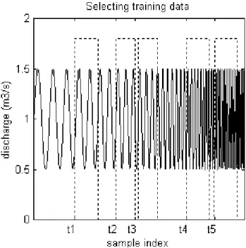
Fig. 3. Example of starting index for five subsets in training data.

4 Model experiment

The input for the ANN is the upstream discharge model boundary which varies between 0.5 and 1.5 m3/s to cover the input space. Within these limits the discharge model bound-ary frequency increases from days to hours in order to en-capsulate enough floods of different durations. It is a sin-function with a decreasing time period resulting in a quick oscillation at the end. The training target of the ANN is the discharge in the central area of the model. The target val-ues are calculated in the numerical flow model. The input and output values will be used to design a data-driven model apart from the physically-based flow model. ANN are used because it is a widely used trend and proved to be an accurate regression method. Alternative methods are for example lin-ear regression methods or model trees (Solomatine and Du-lal, 2003).

A stepped delay line is used to simulate stream flow dy-namics. In a stepped delay line the input at time t until n steps in history Qt −nform the ANN’s input layer (see Fig. 2).

The target values are the flow model’s output at time t . For the ANN we used two inputs; the 2nd and 7th time step of the upstream discharge model boundary in a stepped delay line. These steps were selected based on the cross-correlation graph of input and output data (see Fig. 7). The 2nd time step corresponds with the average travel time of a wave along the shortest route. In the cross-correlation graph there is plat-form at the 7th time step which could correspond to alterna-tive ways for the wave to travel through the flow model. The ANN has two hidden layers with three neurons and five neu-rons respectively and an output layer with one neuron with

(5)

Fig. 4. Training set optimised by Genetic Algorithm.

Fig. 5. Distribution data points of optimised training sets in

com-parison to initial data set.

a linear transfer function. The neurons in the hidden layers have logsig transfer functions.

The network structure, training algorithms, neuron func-tions and other ANN parameters are chosen on the basis of other hydraulic ANN model designs and experiences. It is a general problem that ANN has many design parameters that must be chosen and optimised. Therefore it is in general not straightforward to design a good structure for an ANN; a few rules of thumb for ANN in hydrinformatics were found by Zijderveld (2003). Other hydraulic ANN model designs and experiences were used as a first start. Another general prob-lem of ANN is overfitting. Overfitting means that the training algorithm adjustst the weights of the ANN to fit every single data value in the dataset and at the same time decreases its ca-pability to generelise future, new datasets. To prevent over-fitting, a dataset from a situation for which the desired output

Table 1. Testresults of optimised training set vs standard training

(10 runs).

Testset optimised training (rmse) standard training (rmse)

Test 1 0.0085 0.0114

Test 2 0.0095 0.0134

Test 3 0.0043 0.0124

is known, is used in the training method. If the validation er-ror increases while the training erer-ror steadily decreases then a situation of overfitting may have occurred and the training is stopped.

It is necessary to test the ANN on test sets that relate to hydraulic situations. The method of randomization of test sets was not used because it would not allow blocks of data. For that reason the test set was created distinctly from the training set. The test sets represent different hydrological sit-uations with variations in the hydrograph. The trained ANN will be used as an emulated flow model which, in concept, can simulate every flow condition. For this reason the test-ing was extended to three test sets, see Table 1. Each test set represents a situation with discharge variations with dif-ferent time periods. These three test sets together cover most discharge variations of the flow model.

In this paper the GA is used to optimise the training data to get a better trained ANN. The GA is trained for 30 genera-tions each with 10 off-spring which is a small number. Some calculations with a higher number did not give lower errors. From the initial training set five subsets of equal length (150 data points) are selected. Only the starting point or starting index is chosen by the GA (see Fig. 3). The five subsets to-gether form a new training set with new input/output time series and have a total length of 757 data points wich is half the length of the original training set.

With the combined training set, the ANN makes a new calculation, resulting in a better performing ANN model (RMSE). Based on these results the GA starts the next run and chooses five new samples.

5 Conclusions

For many reasons sufficient and representative data is not always available. In this case we focused on a hydraulic flow model and presumed there is not enough data to train an ANN and decided to produce an artificial dataset. There-fore a dataset was composed regarding the properties of the flow network such as water depth, average discharge and timescales. With this dataset the ANN simulated the target model output which gave, as expected, poor results.

The GA was used to improve the results of the ANN by optimising the original training set. The GA constructed a

(6)

Fig. 6. Frequency spectrum of optimised training set.

new training set by selecting different subsets from the orig-inal training set. The ANN was then trained again with this new training set. This was repeated until the GA found an op-timal training set that performed much better than the initial training set. In this particular flow model it gave on average 39% better results when measured in RMSE. Figure 4 shows one of the resulting training sets. The sharp edges in the dis-charge indicate the borders of the subsets and have no special meaning.

To take a closer look to the resulting dataset, Fig. 5 shows the distribution of the data points in comparison with the original, non optimised training set. A high density means the training set constructed with the GA chose that particu-lar data point frequently. It shows which part of the origi-nal training set is represented by the optimised training set. The GA used data from the entire, original dataset consist-ing of 1489 data samples to find an optimised trainconsist-ing set, except for the first 77 and the last 372 samples. In the last area the frequencies of the discharge is very high as shown in Fig. 3. The explanation for this is that in the flow model quick changes result in an almost constant discharge in the center of the model. The effect is that the relation between inputs and outputs is not ambiguous anymore. An ANN can-not handle this. As a result the GA did can-not select this area in the optimised training set. Slower changes were no problem for the ANN except for the very first samples where noise, induced by initial conditions, influenced the results.

It is also interesting to look at the frequency distribution of the initial and the optimal frequency dataset as shown in Fig. 6. The initial dataset puts emphasis on waves with a time period of half a day. The optimised dataset has corrected this and put more emphasis on a broader spectrum with wave periods from 2.7 days to 14 h. Wave periods longer than 2.7 days (left part of the graph) were excluded in the optimised

Fig. 7. Cross-correlation input and output discharge.

dataset. The GA created a more balanced training set. The optimized training and test sets correspond to a specific flow model and are not universal applicable for other flow models. For each new flow model a new initial training and test set is necessary.

In this paper a GA was used to optimise the training data resulting in a better ANN simulating an existing hydraulic flow model in Baambrugge, The Netherlands. The resulting training data was built from five subsets selected by the GAs optimisation technique and resulted in an ANN which gives more accurate outputs. Further recommendation is to compare this method to other splitting algorithm methods.

Edited by: D. Solomatine

References

Anctil, F. and Lauzon, N.: Generalisation for neural networks through data sampling and training procedures with applications to streamflow predictions, Hydrol. Earth Syst. Sci., 8, 940–958, 2004,

http://www.hydrol-earth-syst-sci.net/8/940/2004/.

Babovic, V. and Keijzer, M.: Genetic programming as a model in-duction engine, J. Hydroinformatics, 2(1), 35–60, 2000. Babovic, V. and Abbott, M. B.: The evolution of equations from

hydraulic data: Part I – Theory, J. Hydraulic Res., 35, 3, 1–14, 1997.

Bowden, G. J., Holger, R. M., and Dandy, G. C.: Optimal division of data for neural network models in water resources applica-tions, Water Resour. Res., 38(2), 1–11, 2002.

Dibike, Y. B.: Model Induction from Data: Towards the next gener-ation of computgener-ational engines in hydraulics and hydrology, IHE Delft, Delft, 2002.

Doan, C. D., Liong, S. Y., and Karunasinghe, D. S. K.: Derivation of effective and efficient dataset with subtractive clustering method and genetic algorithm, J. Hydroinformatics, 7, 219–233, 2005.

(7)

Feyen, L., V´azquez, R., Christiaens, K., Sels, O., and Feyen, J.: Application of a distributed physically-based hydrological model to a medium size catchment, Hydrol. Earth Syst. Sci., 4, 47–63, 2000,

Goldberg, D. E.: Genetic Algorithms in Search, Optimization, and Machine Learning, Addison-Wesley Pub. Co., 1989.

Hagan, T., Demuth, H. B., and Beale, M. H.: Neural Network De-sign, PWS Pub. Co., Boston, 1996.

Haykin, S.: Neural Networks, a comprehensive foundation, Pren-tice Hall, New Jersey, 1999.

Houck, C., Joines, J., and Kay, M.: A genetic algorithm for function optimization: a MATLAB implementation, NCSU-IE TR, 1995. Jolankai, G.: The Tisza River Project, Real-life scale integrated catchment models for supporting water- and environmental man-agement decisions, Section 6 Report, Hungary, 2004.

Minns, A. W. and Hall, M. J.: Artificial neural networks as rainfall-runoff models, Hydrol. Sci. J., 41(3), 399–417, 1996.

Minns, A. W.: Subsymbolic methods for data mining in hydraulic engineering, J. Hydroinformatics, 2, 3–13, 2000.

Price, R. K., Samedov, J. N., and Solomatine, D. P.: An artificial neural network model of a generalised channel network, Proc. 3rd Int. conf. Hydroinformatics, Copenhagen, 1998.

Shannon, C., Moore, D., Keys, K., Fomenkov, M., Huffaker, B., and Claffy, K.: The internet measurement data catalog, Computer communication review, 35, 97–100, 2005.

Shrestha, R. G., Theobald, S., and Nestmann, F.: Simulation of flood flow in a river system using artificial neural networks, Hy-drol. Earth Syst. Sci., 9, 313–321,

Solomatine, D. P. and Dulal, K. N.: Model trees as an alternative to neural networks in trainfall-runoff modelling, Hydrol. Sci. J., 48, 3, 399–411, 2003.

de Vos, N. J. and Rientjes, T. H. M.: Constraints of artificial neural networks for rainfall-runoff modelling: trade-offs in hydrological state representation and model evaluation, Hydrol. Earth Syst. Sci., 9, 111–126, 2005,

Whigham, P. A. and Crapper, P. F.: Modelling rainfall-runoff using genetic programming, Mathematical and Computer Modelling, 33(6–7), 707–721, 2001.

Zijderveld, A.: Neural network design strategies and modelling in hydroinformatics, Ph.D. thesis, Delft University of Technology, Delft, 2003.