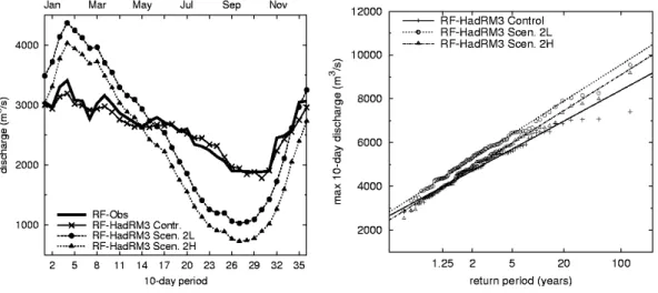
Estimates of future discharges of the river Rhine using two scenario methodologies: direct versus delta approach

The focus of this paper is on the changes in the frequency of extreme droughts under different global warming levels over China by using two large ensemble simulations from the

encourage the ontology engineering community, and more broadly the semantic web community, “to enforce their research efforts by developing further standard criteria [...] and

For energy companies, issues related to the factory of the future are the decentralised production of energy mainly based on renewable energies, the monitoring and

Since the Zimbardo Time Perspective Inventory (ZTPI), an important body of research emerges on the Time Perspective (TP) construct and more specifically on the Future Time

This paper has developed a negotiation scenario to simulate prod- uct’s routing sheet based on the media input of the TRACILOGIS test-bed platform and compare

The present paper is devoted to the computation of two-phase flows using the two-fluid approach. The overall model is hyperbolic and has no conservative form. No instanta- neous

In fact, the number of entrepreneurship education programs has shown an impressive progression in all countries, and this boom in pedagogical programs was supported by

[ 9 ] The differential reactions of the two lakes is due to complex interplays between local climatic conditions and two main lake characteristics: (i) the individual lake mor-