A Method for Automatic and Rapid Mapping of Water Surfaces from Sentinel-1 Imagery

(1)

HAL Id: hal-03060443

https://hal.archives-ouvertes.fr/hal-03060443

Submitted on 17 Dec 2020

HAL is a multi-disciplinary open access

archive for the deposit and dissemination of

sci-entific research documents, whether they are

pub-lished or not. The documents may come from

teaching and research institutions in France or

abroad, or from public or private research centers.

L’archive ouverte pluridisciplinaire HAL, est

destinée au dépôt et à la diffusion de documents

scientifiques de niveau recherche, publiés ou non,

émanant des établissements d’enseignement et de

recherche français ou étrangers, des laboratoires

publics ou privés.

A Method for Automatic and Rapid Mapping of Water

Surfaces from Sentinel-1 Imagery

Filsa Bioresita, Anne Puissant, André Stumpf, Jean-Philippe Malet

To cite this version:

Filsa Bioresita, Anne Puissant, André Stumpf, Jean-Philippe Malet. A Method for Automatic and

Rapid Mapping of Water Surfaces from Sentinel-1 Imagery. Remote Sensing, MDPI, 2018, 10 (2),

pp.217. �10.3390/rs10020217�. �hal-03060443�

(2)

Article

A Method for Automatic and Rapid Mapping of

Water Surfaces from Sentinel-1 Imagery

Filsa Bioresita1,2, Anne Puissant1,*, André Stumpf3and Jean-Philippe Malet3,4 ID 1 _{Laboratoire Image, Ville, Environnement—LIVE/CNRS UMR 7362, Department of Geography,}

University of Strasbourg, 3 rue de l’Argonne, 67000 Strasbourg, France; filsa.bioresita@etu.unistra.fr or filsa.bioresita@gmail.com

2 _{Department of Geomatics Engineering, Institut Teknologi Sepuluh Nopember, Surabaya 60111, Indonesia} 3 _{École et Observatoire des Sciences de la Terre—EOST/CNRS UMS 830, University of Strasbourg,}

67084 Strasbourg, France; andre.stumpf@unistra.fr (A.S.); jeanphilippe.malet@unistra.fr (J.-P.M.)

4 _{Institut de Physique du Globe de Strasbourg—IPGS/CNRS UMR 7516, University of Strasbourg,}

67084 Strasbourg, France

* Correspondence: anne.puissant@live-cnrs.unistra.fr; Tel.: +33-3-68-85-09-15 Received: 19 December 2017; Accepted: 29 January 2018; Published: 1 February 2018

Abstract:Reliable information about the spatial distribution of surface waters is critically important in various scientific disciplines. Synthetic Aperture Radar (SAR) is an effective way to detect floods and monitor water bodies over large areas. Sentinel-1 is a new available SAR and its spatial resolution and short temporal baselines have the potential to facilitate the monitoring of surface water changes, which are dynamic in space and time. While several methods and tools for flood detection and surface water extraction already exist, they often comprise a significant manual user interaction and do not specifically target the exploitation of Sentinel-1 data. The existing methods commonly rely on thresholding at the level of individual pixels, ignoring the correlation among nearby pixels. Thus, in this paper, we propose a fully automatic processing chain for rapid flood and surface water mapping with smooth labeling based on Sentinel-1 amplitude data. The method is applied to three different sites submitted to recent flooding events. The quantitative evaluation shows relevant results with overall accuracies of more than 98% and F-measure values ranging from 0.64 to 0.92. These results are encouraging and the first step to proposing operational image chain processing to help end-users quickly map flooding events or surface waters.

Keywords:surface waters; floods; Sentinel-1; automatic thresholding method; filtering

1. Introduction

Mapping the extent of surface waters is crucial for many applications as waters constitute a resource and a natural hazard during flooding events. Flood disasters occur in many regions of the globe and cause great losses each year [1], and flood extend maps derived from optical or Synthetic Aperture Radar (SAR) Earth Observation (EO) sensors are a source of information for flood disaster management [2]. Besides disaster relief operations, these maps can also serve for the validation of hydraulic models [3–5] and for quantifying flood hazard maps in the context of spatial planning and insurance [6].

In the case of favorable weather conditions, optical EO sensors are the preferred information source due to their straightforward interpretability. Successful applications of optical satellite data are presented in [7,8], while a detailed review of optical-based flood mapping is presented in [9].

However, as flood events often occur during periods of persistent cloud cover, monitoring by optical sensors (visible, infrared, thermal) is rarely feasible. Microwave SAR sensors offer clear advantages by providing their own sources of illumination, thus being able to operate in nearly all-weather/day-night Remote Sens. 2018, 10, 217; doi:10.3390/rs10020217 www.mdpi.com/journal/remotesensing

(3)

Remote Sens. 2018, 10, 217 2 of 17

conditions. For almost 20 years, spaceborne SAR sensors have increasingly been used for large-scale flood mapping, mainly at medium spatial resolutions, using X- (SIR-C/X-SAR, SRTM), C- (ERS-1/2 AMI, Envisat ASAR, RADARSAT-1, RISAT-1, SIR-C/X-SAR), and L- (SEASAT-1, JERS-1, ALOS PALSAR, SIR-A/B/C/X-SAR) band sensors. With the launch of the X-band TerraSAR-X/TanDEM-X and COSMO-SkyMed (CSK) constellations, higher sensor spatial resolutions (up to 0.24 m for the TerraSAR-X Staring SpotLight mode) or higher revisit times (six days for Sentinel-1, and up to 5×20 m in the standard Interferometric Wide—IW—Swath mode), have increased capabilities for estimating flood extent and for flood monitoring in the case that complex, small-scale, and operational scenarios are available. The potential of this new generation X-band data has already been demonstrated by several use cases in flood emergency situations [10–12]. The usefulness of the C-band Sentinel-1 sensor mission for flood mapping purposes has not been thoroughly investigated, while the design of this mission for operating in a pre-programmed conflict-free mode ensuring consistent long-term data archives [13] and the possibility of fully-automated surface water services [14] have been studied. The objective of this work is to address this gap by investigating the potential of Sentinel-1 data for the efficient and reliable mapping of flood extents.

Several SAR-based water detection algorithms have been proposed in the literature using supervised and unsupervised classification approaches [15–17], thresholding [18–20], object-based image analysis [21,22], and hybrid approaches [23,24]. Among these methods, thresholding is the most commonly adopted method for SAR image analysis to discriminate water and non-water areas. The approach is based on the contrast of low radar returns from water bodies and high radar returns from the surrounding terrain. The accuracy of the detection algorithms varies drastically independent of the land cover prevalent in the scene. Flood detection in urban areas is very challenging due to shadowing effects from buildings as a result of the side-looking viewing geometry of SAR satellite sensors [25]. Further, waters beneath vegetation layers are difficult to detect due to double bounce scattering resulting in a drastic increase of radar backscatter in such areas [26]. Misclassification errors are also prevalent in the presence of strong wind that roughens the water surfaces. Finally, it is difficult to determine the optimal threshold value for a scene/landscape, which implies the need for user intervention.

The number of SAR-based water detection algorithms and automatic flood mapping services has increased in the last years [3,19,27]. In most cases, a certain amount of user interaction is needed for data collection, pre-processing, and integration of auxiliary data in the processing pipelines. NASA’s Goddard’s Office of Applied Science proposes an automated global daily flood and surface water mapping service (http://oas.gsfc.nasa.gov/floodmap/). As one of the first SAR-based services, the Fast Access to Imagery for Rapid Exploitation (FAIRE) service hosted on the ESA’s Grid Processing on Demand system (G-POD,http://gpod.eo.esa.int/) provides automatic SAR pre-processing and change detection capabilities which can be triggered on demand by a user via a web-interface. Automatic algorithms for medium resolution surface water mapping have been presented by [28], e.g., Fully Automatic Aqua Processing Service/FAAPS) and [29]. WaMaPro [30] implements thresholding and morphological filtering but requires user intervention. RaMaFlood [31] has been developed for semi-automatic flood extent mapping using an interactive object-based classification algorithm. The TerraSAR-X Flood Service (TFS) [25] and the TanDEM-X Water Indication Mask processor (TDX WAM) [31] are water detection tools based on fully-automatic processing of TerraSAR-X and TanDEM-X images. The Canada Centre for Remote Sensing has developed the FnFCE (Forest non-Forest Class Extraction) water detection tool for the automated extraction of water bodies, but this tool only ingests Radarsat images [32].

The processing chain of the TerraSAR-X Flood Service is currently being adapted to Sentinel-1 data [33], which enables systematic disaster monitoring with high spatial and temporal resolutions. In contrast to the TerraSAR-X Flood Service, this is a major advantage since the time-consuming step of tasking new satellite data can be omitted.

Hence, while several semi-automatic and automatic tools already exist, there are, to the best of our knowledge, currently only a few scientific references which present a fully automatic water detection

(4)

processor for surface water mapping from Sentinel-1 imagery [33–35]. This method uses thresholding on individual pixels ignoring the correlation among neighboring pixels. Considering that individual pixels are not independent random variables but form a random field [36], the potential to improve the accuracy of the flood extent maps exists.

The objectives of this work are thus (1) to investigate the use of bilateral filtering as a smooth labeling method for defining the thresholds; (2) to integrate hydrologic/topographic information in the detection using the ‘Height above nearest drainage’ (HAND) index [37]; and (3) to quantitatively evaluate the accuracy of our proposed fully-automated SAR-based water detection algorithm for Sentinel-1 data.

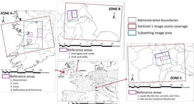
2. Study Areas and Datasets

Three test areas were selected for this study as shown in Table1. During Storm Desmond on the 4 December 2015, heavy rain with a 24 h total of 160.8 mm was reported at Keenagh Beg (Co Mayo, Ireland) [38]. The storm led to a 100-year flood event particularly affecting the cities Ennis, Gort, Roscommon, Ballinasloe, and Portumna (Figure1—Zone A).

Table 1.Images used, location, and events.

No

Occasion

SAR Acquisition Mode

Zone Image Acquisition Information

1

Zone A (Ireland)

22 November 2015 Before floods Ascending

2 16 December 2015 Floods occurred Ascending

3 9 January 2016 Floods occurred Ascending

4 14 February 2016 After floods Ascending

5 Zone B (England) 29 December 2015 Floods occurred Descending 6 Zone C (Italy) 28 November 2016 Floods occurred Ascending

Three weeks after, heavy rainfalls (about 215 mm 24 h rainfall) during Storm Eva (22 December 2015) caused flooding to areas in Northern England [39]. Particularly affected areas were Yorkshire, along the River Ouse, and a large zone of West Yorkshire including the city of Leeds (Figure1—zone B). Starting on 21 November 2016, persistent rainfalls with levels of up to 200 mm in around 12 h were recorded in some areas of North West Italy [40]. This led to severe flooding in the regions Liguria and Piedmont (Figure1—zone C).

Six images of Sentinel-1 IW GRDH (Ground Range Detected in High resolution) data are available for these three study sites. Sentinel-1 imageries include pre-event, during event, or post-event images collected from the European Space Agency (ESA) Sentinels Scientific Data Hub [41]. Each image has a spatial resolution of about 20×22 m with double polarization (VV and VH). In order to build HAND (Height above Nearest Drainage) [42] maps to account for the limitation of surface water areas, SRTM (Shuttle Radar Topography Mission) version 3, 1 Arc-Second Global with a 30-m resolution is used [43].

Reference maps to assess our results are available through the COPERNICUS Emergency Management Service [44]. These data are produced using ESRI World Imagery, COSMO-SkyMed, Radarsat-2, and other images except Sentinel imagery [44].

A preliminary statistical analysis based on permanent surface water surfaces in the Alsace Region (France) defined by topographic databases showed that with the spatial resolution of SENTINEL-1 images, the smallest water surfaces are limited to 1 ha. Consequently, only areas greater than or equal to 1 ha will be retained in the reference maps for the quantitative assessment.

(5)

Remote Sens. 2018, 10, 217 4 of 17

Remote Sens. 2018, 10, x FOR PEER REVIEW 4 of 18

Remote Sens. 2018, 10, x; doi: FOR PEER REVIEW www.mdpi.com/journal/remotesensing Figure 1. Study areas: Zone A—Ireland, Zone B—England and Zone C—Italy.

3. Methods

The automatic processing chain is described in Figure 2. It includes five components: (i) pre-processing of raw Sentinel-1 data; (ii) a tiling approach in order to focus on surface water areas automatically; (iii) class modeling with Finite Mixture Models [45] to produce probability maps based on established class models; (iv) bilateral filtering [36] for smooth labelling; and (v) post-processing and accuracy assessment.

In this study, we try to compare two scenarios of the processing chain based on the use of the HAND map. In the first scenario, the HAND index is applied in the pre-processing step to limit the considered area for the next processing step in order to avoid misclassification. In the second scenario, the HAND index is used as a final post-processing step for the amount of misclassified areas in the surface water maps. Moreover, we also perform a sensibility analysis of tile size used for the tiling approach in order to find a suitable tile size to be used in the processing.

Figure 2. Flowchart showing the overall methods used in this study. Figure 1.Study areas: Zone A—Ireland, Zone B—England and Zone C—Italy. 3. Methods

The automatic processing chain is described in Figure2. It includes five components: (i) pre-processing of raw Sentinel-1 data; (ii) a tiling approach in order to focus on surface water areas automatically; (iii) class modeling with Finite Mixture Models [45] to produce probability maps based on established class models; (iv) bilateral filtering [36] for smooth labelling; and (v) post-processing and accuracy assessment.

Remote Sens. 2018, 10, x; doi: FOR PEER REVIEW www.mdpi.com/journal/remotesensing Figure 1. Study areas: Zone A—Ireland, Zone B—England and Zone C—Italy.

3. Methods

The automatic processing chain is described in Figure 2. It includes five components: (i) pre-processing of raw Sentinel-1 data; (ii) a tiling approach in order to focus on surface water areas automatically; (iii) class modeling with Finite Mixture Models [45] to produce probability maps based on established class models; (iv) bilateral filtering [36] for smooth labelling; and (v) post-processing and accuracy assessment.

Figure 2. Flowchart showing the overall methods used in this study. _{Figure 2.}_{Flowchart showing the overall methods used in this study.}

(6)

3.1. Processing Chain

3.1.1. Step 1: Pre-Processing

Image pre-processing is applied to each Sentinel-1 IW GRDH dataset in order to reduce orbital errors, speckle noise, and geometric distortion. A first processing step comprises the application of precise Sentinel orbits, which can be obtained from SNAP (Sentinel Application Platform) [46,47] and considerably improve the geolocation accuracy. To transform raw amplitude images to calibrated products for the quantitative use of SAR images, we used also SNAP software. Among available calibrated products from SNAP, such as amplitude, intensity, beta-nought, and sigma nought, we selected sigma-nought since preliminary statistical tests showed that sigma-nought provides a better separation between water and land surfaces. Some previous studies have also used sigma-nought images for surface water mapping [48,49]. In order to reduce speckle noise, multilooking and speckle filtering with a Median filter and window size of 5×5 pixels was used after some preliminary tests on the size of window (3×3 or 5×5) and with some types of filtering (Mean, Median, Gamma Map, Lee, Frost, and Refined Lee). Subsequently, Range Doppler Terrain Correction was applied to geocode the images.

3.1.2. Step 2: Image Tiling Using a Modified Split-Based Approach (MSBA)

A Split-Based Approach (SBA) was originally proposed by [50] for flood detection with Radarsat images. This approach comprises a tiling of the satellite imagery into smaller sub scenes of a user-defined size and a successive local thresholding analysis. The approach’s performance has been confirmed in many studies for automatic mapping in remote sensing, e.g., [19,51]. The original SBA approach relies on the coefficient of variation to pre-select tiles for further processing and a global thresholding method to produce binary maps of surface water coverage. As noted by the authors, global thresholding methods are well adapted for small scene extents but face problems for the larger scene extents of Sentinel-1 with higher backscatter variances resulting from variations in the incidence angle.

To address this issue, we proposed a modified split-based approach which only applied pre-selection tiles for class modelling. Images are first automatically tiled into squared non-overlapping blocks. The tiles selection is then performed to choose only image tiles, which contain some portion of surface waters. This selection is based on Hartigan’s dip statistic (HDS) value [52]. The underlying hypothesis is that tiles with surface waters and land areas have bimodal grey-value distributions. HDS is used to distinguish between tiles with unimodal and bimodal distributions. p-values resulting from the HDS test are considered with values less than 0.05, indicating statistically significant bimodality [52]. Thus, only tiles with a p-value of less than 0.05 will be used for the subsequent class modelling with finite mixture models. In this context, it is important to note that this processing step only concerns the pre-selection for the class modeling, whereas the entire image is processed for the generation of the final water surface maps. 3.1.3. Step 3: Class Modelling with Finite Mixture Models (FMM)

The Finite Mixture Models represent the existence of subclass diversity with a limited number of distributions. They allow the decomposition of probability distributions into subgroups assuming that the observed distribution is the result of a mixture of sub-populations which are distributed according to a particular form (i.e., Gaussian). A popular method for modeling the parameters of the probability distributions contributing to the mixture is Expectation-Maximization (EM) [45]. The experimental results presented in this study rely on the assumption of a mixture of two Gaussian components, whereas the underlying implementation also allows the use of skewed distributions such as the Gamma function. Their initial means are determined automatically from the binned histograms and the standard deviation is set as 3 for the respective tile. The probability of surface waters is set as 0.1 in accordance with previous works [19,53], suggesting that a minimum amount of 10% of each class is sufficient for accurate threshold detection. Sensitivity tests of these parameters are performed to quantify the influence of standard deviation and probability parameters in this process. The EM-based distribution fitting is performed over a maximum of 1000 iterations and tiles for which convergence

(7)

Remote Sens. 2018, 10, 217 6 of 17

is not reached within this number of iterations are excluded only for the calculation of the threshold value. Instead of directly determining the threshold value, this process is used to compute posterior probabilities to generate surface water probability maps.

The standard EM algorithm for normal mixtures is based on a first step called E-step (Equation (1)) and followed by a second step called M-step (Equation (2)) [45]. In the E-step, it searches for the expected value p of the complete likelihood for all i = 1, . . . , n and j = 1, . . . , m at iteration t, from the given parameterization (λ, φ(x)). p(_ijt)=  1+

∑

j06=j λ(_j0t)φ (t) j0 (xi) λ(_jt)φ(_jt)(xi)   −1 (1) In the M-step, it finds the model parameters λ that maximize the conditional expected values from the E-step.

λ(_jt+1) =1 n n

∑

i=1 p(_ijt), for j=1, . . . , m (2)

After computing the model parameters for each tile, we calculate the average of those parameters to derive a global set of parameters. Then, using the global parameters, posterior probabilities (Equation (1)) are computed for each pixel of the entire image.

3.1.4. Step 4: Smooth Labelling Using a Bilateral Filtering Approach

Binary thresholding methods commonly treat each pixel independently to assign class labels such as land and surface water areas. However, considering the spatial auto-correlations among nearby pixels, it can be assumed that nearby pixels tend to have the same class label (smoothness assumption) [36].

Based on this assumption, bilateral filtering is used as a strategy for smooth labelling and the suppression of small spurious detection. This filter is a non-linear, edge-preserving, and noise-reducing smoothing filter commonly used in image processing. The intensity value at each pixel in an image is replaced by a weighted average of intensity values from nearby pixels. The resulting image is subsequently transformed into a binary image assigning all pixels with a probability of surface water greater than 0.9 as water surface.

3.1.5. Step 5: Post-Processing

In the post-processing step, the accuracy of final binary maps is assessed by calculating classical measures (overall accuracy, F-measure [54], true positive rates, false positive rates, omission and commission errors) obtained by a comparison with very-high resolution Copernicus products [44]. 3.2. Comparison of Two Scenarios Using HAND Maps

Height above Nearest Drainage (HAND) is a terrain index based on the drainage network [42,55]. A previous study showed the advantages of using HAND maps for flood mapping [33,34] to remove false positive surface water detections which are located high above the nearest drainage line. In order to create HAND maps, stream networks are defined with a 10 ha threshold [56]. For this study, a HAND threshold of 15 m [33,42] is used.

In this study, we performed two approaches to improve the accuracy of the surface water mapping. The first approach is using the HAND map in the pre-processing step, while the second approach employs the HAND map in the post-processing step. A comparison of the results will determine the best scenario for this study. A tile size of 10 km will be used in both of the scenarios.

(8)

3.2.1. Scenario 1: Use of HAND Maps in Pre-Processing

For the first scenario, we use a HAND map in the pre-processing step, after subsetting the sigma-nought image in the study area boundary. All areas with a HAND index of >15 m are excluded from all further processing steps including the computation of the HDS, finite mixture modelling, the generation of the probability maps, bilateral filtering, and the generation of the final maps. In this scenario, potential false positives are removed in the initial stage of the processing chain and will thus not impact the statistical analysis. A further advantage of this scenario is the reduction of the amount of data and hence faster processing.

3.2.2. Scenario 2: Use of HAND Maps in Post-Processing

In the second scenario, we use a HAND map only in the post-processing step after labeling the surface water class. In order to reduce misclassification, we subset surface water areas in the HAND≤15 m boundaries and produced the final surface waters map. In this scenario, all previous processing steps are based on the entire input image.

3.3. Sensitivity Analysis of Tile Size Used in Tiling Approach

It is a known issue that statistical thresholding methods applied to subsets of the image are sensitive to the size of the individual tiles [19]. The default tile size used in this study is 10×10 km due to the spatial extent of a Sentinel-1 image (250 km swath), but it cannot be excluded that increasing or reducing the tile size might improve or degrade the accuracy of the final maps. Using the first processing scenario, tile sizes of 2.5 km and 5 km are also evaluated and compared for the three zones (A, B, and C).

4. Results

4.1. Influence of FMM Parameters Values

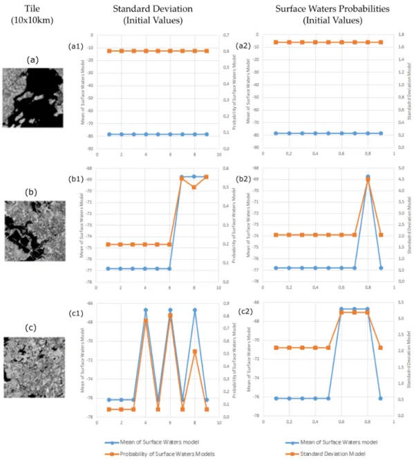
Given that FMMs are sensitive to the initial values set for standard deviations and prior class probabilities, the impact of variations in the initial parameter settings on the final class model is examined. The influence of FFM parameter values is assessed for the Sentinel-1 image (9 January 2016). This analysis is performed for three tiles of Zone A (Ireland), which are representative for different proportions of land and surface waters (Figure3). In Tile (a), surface waters cover more than 70% of the area, while in Tile (b), land and surface waters cover the same proportion of areas. In Tile (c), the majority is land surface. FMMs are initialized on these three tiles testing initialization values from 1 to 9 and from 0.1 to 0.9 for the standard deviation and prior class probabilities, respectively.

The results of this evaluation are presented in Figure3. In the column of standard deviation, we give various values of standard deviation as initial values and observe mean and probability values of the model. The graphs indicate the mean and probability values of the model associated with initial values of standard deviation. Subsequently, in the column of surface water probabilities, we give various values of probability as initial values and observe mean and standard deviation values of the model. Figure3shows that image tiles with large portions of surface water areas converge to the same stable output model no matter which initial values are selected. Contrarily, Tile (c), which includes rather small portions of surface water area, tends to marginal solutions at standard deviations above 3 or prior probabilities for the surface water class above 0.5. For Tile (b), which presents an intermediate contribution of water surfaces, the FMMs converge to a stable solution below standard deviations of 7 and water class probabilities of 0.7. Considering the results of this analysis, the use of a standard deviation of 3 and prior probability of 0.1 was considered as sufficiently low to assure that the FMMs will generally converge to stable solutions with a good approximation of the bimodal distributions.

(9)

Remote Sens. 2018, 10, 217 8 of 17

Remote Sens. 2018, 10, x; doi: FOR PEER REVIEW www.mdpi.com/journal/remotesensing Figure 3. Variation of standard deviation (a1,b1,c1) and surface water probabilities (a2,b2,c2) in the initial values of FMM parameters to output models for different proportions of land and surface waters in tiles.

The results of this evaluation are presented in Figure 3. In the column of standard deviation, we give various values of standard deviation as initial values and observe mean and probability values of the model. The graphs indicate the mean and probability values of the model associated with initial values of standard deviation. Subsequently, in the column of surface water probabilities, we give various values of probability as initial values and observe mean and standard deviation values of the model. Figure 3 shows that image tiles with large portions of surface water areas converge to the same stable output model no matter which initial values are selected. Contrarily, Tile (c), which includes rather small portions of surface water area, tends to marginal solutions at standard deviations above 3 or prior probabilities for the surface water class above 0.5. For Tile (b), which presents an intermediate contribution of water surfaces, the FMMs converge to a stable solution below standard deviations of 7 and water class probabilities of 0.7. Considering the results of this Figure 3.Variation of standard deviation (a1,b1,c1) and surface water probabilities (a2,b2,c2) in the initial values of FMM parameters to output models for different proportions of land and surface waters in tiles. 4.2. Sensitivity of Bilateral Filtering Parameter

The size of the filtering window and its influence on the results is also analyzed. The sensitivity of the classification accuracy to changes in these parameters is evaluated empirically for the image Sentinel-1 scene recorded on 9 January 2016 over the Gort area in Zone A.

Figure4represents the dependence of overall accuracy and F-measure on changes in the window size. It can be seen that a window size of 5×5 pixels yields the optimal result with the overall accuracy reaching 99.07% and F-measure at 0.84. Therefore, for all experiments, the bilateral filtering window was fixed to 5×5 pixels.

(10)

Remote Sens. 2018, 10, 217 9 of 17

Remote Sens. 2018, 10, x; doi: FOR PEER REVIEW www.mdpi.com/journal/remotesensing analysis, the use of a standard deviation of 3 and prior probability of 0.1 was considered as sufficiently low to assure that the FMMs will generally converge to stable solutions with a good approximation of the bimodal distributions.

4.2. Sensitivity of Bilateral Filtering Parameter

The size of the filtering window and its influence on the results is also analyzed. The sensitivity of the classification accuracy to changes in these parameters is evaluated empirically for the image Sentinel-1 scene recorded on 9 January 2016 over the Gort area in Zone A.

Figure 4 represents the dependence of overall accuracy and F-measure on changes in the window size. It can be seen that a window size of 5 × 5 pixels yields the optimal result with the overall accuracy reaching 99.07% and F-measure at 0.84. Therefore, for all experiments, the bilateral filtering window was fixed to 5 × 5 pixels.

Figure 4 also shows that bilateral filtering yields higher overall accuracies when compared to unfiltered maps over a wide range of window sizes between 3 × 3 pixels and 17 × 17 pixels. This clearly justifies the use of a bilateral filter as the smooth labeling method in this study.

(a) (b)

Figure 4. Dependence of classification result on bilateral filter window size indicated (a) by overall accuracy and (b) F-measure value.

4.3. Results Comparison between Scenario 1 and Scenario 2

Based on a comparison of quantitative evaluation results from scenario 1 and 2, there are no significant differences in all evaluation parameter values between the two scenarios. However, compared to scenario 2, scenario 1 gives slightly better evaluation results. This can be seen in Figure 5, which displays the F-measure values from all images. In the F-measure graph, the higher the value signifies the better the results. Figure 5 shows higher values for scenario 1 for two images and the same values for the other images. Thus, the use of scenario 1 is recommended and will be applied for this study.

Figure 4.Dependence of classification result on bilateral filter window size indicated (a) by overall accuracy and (b) F-measure value.

Figure4also shows that bilateral filtering yields higher overall accuracies when compared to unfiltered maps over a wide range of window sizes between 3×3 pixels and 17×17 pixels. This clearly justifies the use of a bilateral filter as the smooth labeling method in this study.

4.3. Results Comparison between Scenario 1 and Scenario 2

Based on a comparison of quantitative evaluation results from scenario 1 and 2, there are no significant differences in all evaluation parameter values between the two scenarios. However, compared to scenario 2, scenario 1 gives slightly better evaluation results. This can be seen in Figure5, which displays the F-measure values from all images. In the F-measure graph, the higher the value signifies the better the results. Figure5 shows higher values for scenario 1 for two images and the same values for the other images. Thus, the use of scenario 1 is recommended and will be applied for this study.

Remote Sens. 2018, 10, x; doi: FOR PEER REVIEW www.mdpi.com/journal/remotesensing Figure 5. Comparison of F-measure between scenario 1 and 2 for all images.

4.4. Sensitivity of Tile Size in MSBA and FMM Steps

A sensitivity analysis is carried out in all study areas through a quantitative assessment of the results with different tile sizes. Using scenario 1 and all further processing steps as explained above, only the tile size used in the MSBA and FMM steps is changed to values of 10 km, 5 km, and 2.5 km. A quantitative comparison against the available reference maps in Zone A is presented in Table 2 and indicates only subtle differences between three tile sizes. While small variations exist regarding the tradeoff between TPR and FPR, the F-measures are indistinguishable.

Table 2. Results assessment for three different tile sizes in Zone A—Ireland.

Evaluation 22 November 2015 16 December 2015 09 January 2016 14 February 2016 10 km 5 km 2.5 km 10 km 5 km 2.5 km 10 km 5 km 2.5 km 10 km 5 km 2.5 km Overall accuracy 99.41% 99.40% 99.40% 98.68% 98.68% 98.68% 98.68% 98.67% 98.66% 99.35% 99.36% 99.38% F-measure 0.88 0.88 0.88 0.77 0.77 0.78 0.92 0.92 0.92 0.88 0.88 0.88 TPR 81.27% 81.65% 81.44% 66.96% 67.04% 67.83% 89.67% 89.42% 89.18% 86.42% 86.26% 86.51% FPR 0.09% 0.10% 0.10% 0.22% 0.22% 0.24% 0.47% 0.45% 0.44% 0.29% 0.27% 0.31% Omission error 18.73% 18.35% 18.56% 33.04% 32.96% 32.17% 10.32% 10.58% 10.82% 13.58% 13.74% 13.49% Commission error 3.79% 4.29% 4.06% 8.54% 8.60% 9.31% 5.26% 5.10% 4.96% 10.80% 10.22% 11.29%

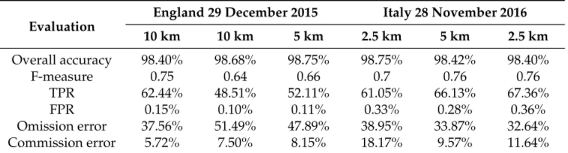
Similarly, in Zone B, a smaller tile size seems to favor both a higher TPR and a higher FPR, whereas the F-measure remains rather stable among all tested tile sizes (Table 3). On the other hand, the results for Zone C indicate a significant improvement from an F-measure of 0.64 towards 0.7 when using smaller tile sizes (Table 3). This might be due to smaller water surfaces in Zone C, which are less likely to be omitted at smaller tile sizes.

Table 3. Results assessment for three different tile sizes in Zone B—England and Zone C—Italy. Evaluation England 29 December 2015 Italy 28 November 2016

10 km 10 km 5 km 2.5 km 5 km 2.5 km Overall accuracy 98.40% 98.68% 98.75% 98.75% 98.42% 98.40% F-measure 0.75 0.64 0.66 0.7 0.76 0.76 TPR 62.44% 48.51% 52.11% 61.05% 66.13% 67.36% FPR 0.15% 0.10% 0.11% 0.33% 0.28% 0.36% Omission error 37.56% 51.49% 47.89% 38.95% 33.87% 32.64% Commission error 5.72% 7.50% 8.15% 18.17% 9.57% 11.64%

Figure 5.Comparison of F-measure between scenario 1 and 2 for all images. 4.4. Sensitivity of Tile Size in MSBA and FMM Steps

A sensitivity analysis is carried out in all study areas through a quantitative assessment of the results with different tile sizes. Using scenario 1 and all further processing steps as explained above,

(11)

Remote Sens. 2018, 10, 217 10 of 17

only the tile size used in the MSBA and FMM steps is changed to values of 10 km, 5 km, and 2.5 km. A quantitative comparison against the available reference maps in Zone A is presented in Table2and indicates only subtle differences between three tile sizes. While small variations exist regarding the tradeoff between TPR and FPR, the F-measures are indistinguishable.

Table 2.Results assessment for three different tile sizes in Zone A—Ireland.

Evaluation

22 November 2015 16 December 2015 09 January 2016 14 February 2016 10 km 5 km 2.5 km 10 km 5 km 2.5 km 10 km 5 km 2.5 km 10 km 5 km 2.5 km Overall accuracy 99.41% 99.40% 99.40% 98.68% 98.68% 98.68% 98.68% 98.67% 98.66% 99.35% 99.36% 99.38% F-measure 0.88 0.88 0.88 0.77 0.77 0.78 0.92 0.92 0.92 0.88 0.88 0.88 TPR 81.27% 81.65% 81.44% 66.96% 67.04% 67.83% 89.67% 89.42% 89.18% 86.42% 86.26% 86.51% FPR 0.09% 0.10% 0.10% 0.22% 0.22% 0.24% 0.47% 0.45% 0.44% 0.29% 0.27% 0.31% Omission error 18.73% 18.35% 18.56% 33.04% 32.96% 32.17% 10.32% 10.58% 10.82% 13.58% 13.74% 13.49% Commission error 3.79% 4.29% 4.06% 8.54% 8.60% 9.31% 5.26% 5.10% 4.96% 10.80% 10.22% 11.29%

Similarly, in Zone B, a smaller tile size seems to favor both a higher TPR and a higher FPR, whereas the F-measure remains rather stable among all tested tile sizes (Table3). On the other hand, the results for Zone C indicate a significant improvement from an F-measure of 0.64 towards 0.7 when using smaller tile sizes (Table3). This might be due to smaller water surfaces in Zone C, which are less likely to be omitted at smaller tile sizes.

Table 3.Results assessment for three different tile sizes in Zone B—England and Zone C—Italy.

Evaluation

England 29 December 2015 Italy 28 November 2016

10 km 10 km 5 km 2.5 km 5 km 2.5 km Overall accuracy 98.40% 98.68% 98.75% 98.75% 98.42% 98.40% F-measure 0.75 0.64 0.66 0.7 0.76 0.76 TPR 62.44% 48.51% 52.11% 61.05% 66.13% 67.36% FPR 0.15% 0.10% 0.11% 0.33% 0.28% 0.36% Omission error 37.56% 51.49% 47.89% 38.95% 33.87% 32.64% Commission error 5.72% 7.50% 8.15% 18.17% 9.57% 11.64% 5. Discussion

Generally, the accuracy assessment shows very high overall accuracies of about 98% for each of the study sites. Moreover, the commission error remains below 20% for all test zones. The final quantitative evaluation of surface water extraction results is presented in Table4. The presented results are obtained fully automatically using scenario 1 and a tile size of 10 km. As shown in the previous section, further improvements can be expected through an adaptation of the tile size, whereas we prefer to present here the results obtained with a default value that is more realistic for an operational scenario. For each zone, a map depicting the extent of surface waters is presented and several zooms overlaying Sentinel-2 imagery allow a better visualization of results. The surface water detection in Zone A shows results with F-measures ranging from 0.77 to 0.92. Figure6a–d show that false negatives occur mainly along the borders of surface water bodies, where most of the false positives are also located. In the Ennis area, the narrow river with a width of around 50 m cannot be detected. This is probably due to vegetation along the river banks and increased turbulence along the permanent riverbed which leads to increased backscattering in those areas (see Figure6d). Flooded areas are detected in wetland areas along Shannon River (Figure6b).

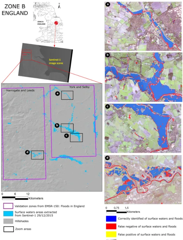
The evaluation of Zone B shows an adequate performance of the automatic detection with an F-measure value of 0.75. Zone B comprises numerous narrow river sections which, even during flooding events, do not exceed 100 m in width and are consequently difficult to detect with Sentinel-1 (see Figure7d). Similar to Zone A, the detection of these sections is further complicated by tree-and hedge lines along the river banks, as well as greater turbulence and hence water surface roughness along the permanent riverbed.

(12)

Zone C comprises several narrow river sections in Sale regions, which similarly leads to omission errors of about 51%. Some false negatives are visible along the borders of Po River (see Figure8a,b) and mostly appear in the bar or river bank areas (see Figure8c,d). In particular, it seems that several bar and river banks already reemerged after the main flooding event on 25 and 26 November 2016. The omission is hence due to the acquisition delay of Sentinel-1 because, at the time of imaging, these areas where not submerged.

Given the persistent omission of permanent river beds at all three study sites, further improvements of the processing chain could include the analysis of SAR time-series to amplify the signal of permanent riverbeds through spatio-temporal averaging.

Considering these results, our new automatic chain processing for floods detection and rapid surface water mapping using Sentinel-1 data appears to be efficient for mapping flood events and water surfaces. It has been applied to three major floods events in Ireland, the United Kingdom, and Italy with largely favorable results. The proposed method features a short processing time. For instance, using a computer with multiple Intel Duo processors of 1.90 GHz and 32 GB RAM, the time of processing is about 10 h per Sentinel-1 image. Multiple images can be processed easily in parallel. Rapid mapping can hence be achieved in less than half a day after the image data is made publicly available. Given the variable landscape characteristics at the investigated sites, we consider that the processing chain can also be deployed for rapid mapping in other geographic regions. Probabilistic map products can also be derived to better guide further intervention by human operators if required.

In this study, the methodology was specifically designed for the analyses of Sentinel-1 data and the suitability of the method for rapid surface water mapping was explored. The method is adapted to the particular features of high spatial resolution Sentinel-1 data which are different from the other available automatic tools targeting the use of SAR images with a very high spatial resolution (e.g., [31,57]). Since the required Sentinel-1 input data is publicly available without restriction, it will be easy to access unlimited data of Sentinel-1 and process it for surface water mapping.

Table 4.Quantitative evaluation of surface water extraction results (using scenario 1 and tile size 10 km). Study

Area Image Date Event

Overall Accuracy F-Measure True Positive Rate False Positive Rate Omission Error Commission Error Zone A (Ireland)

22 November 2015 Before floods 99.41% 0.88 81.27% 0.09% 18.73% 3.79%

16 December 2015 _occurredFloods 98.68% 0.77 66.96% 0.22% 33.04% 8.54%

09 January 2016 _occurredFloods 98.68% 0.92 89.67% 0.47% 10.32% 5.26%

14 February 2016 After floods 99.35% 0.88 86.42% 0.29% 13.58% 10.80%

Zone B (England) 29 December 2015 Floods occurred 98.40% 0.75 62.44% 0.15% 37.56% 5.726 Zone C (Italy) 28 November 2016 Floods occurred 98.68% 0.64 48.51% 0.10% 51.49% 7.50%

(13)

Remote Sens. 2018, 10, 217 12 of 17

Remote Sens. 2018, 10, x; doi: FOR PEER REVIEW www.mdpi.com/journal/remotesensing Figure 6. Surface water extraction result in Zone A (Ireland) with several zoom areas overlaying Sentinel-2.

(14)

Remote Sens. 2018, 10, x; doi: FOR PEER REVIEW www.mdpi.com/journal/remotesensing Figure 7. Surface water extraction result in Zone B (England) with several zoom areas overlaying Sentinel-2 imagery.

Figure 7. Surface water extraction result in Zone B (England) with several zoom areas overlaying Sentinel-2 imagery.

(15)

Remote Sens. 2018, 10, 217 14 of 17

Remote Sens. 2018, 10, x; doi: FOR PEER REVIEW www.mdpi.com/journal/remotesensing Figure 8. Surface water extraction result in Zone C (Italy) with several zoom areas overlaying Sentinel-2 imagery.

Considering these results, our new automatic chain processing for floods detection and rapid surface water mapping using Sentinel-1 data appears to be efficient for mapping flood events and water surfaces. It has been applied to three major floods events in Ireland, the United Kingdom, and Italy with largely favorable results. The proposed method features a short processing time. For instance, using a computer with multiple Intel Duo processors of 1.90 GHz and 32 GB RAM, the time of processing is about 10 h per Sentinel-1 image. Multiple images can be processed easily in parallel. Rapid mapping can hence be achieved in less than half a day after the image data is made publicly available. Given the variable landscape characteristics at the investigated sites, we consider that the processing chain can also be deployed for rapid mapping in other geographic regions. Probabilistic map products can also be derived to better guide further intervention by human operators if required. In this study, the methodology was specifically designed for the analyses of Sentinel-1 data and the suitability of the method for rapid surface water mapping was explored. The method is adapted Figure 8.Surface water extraction result in Zone C (Italy) with several zoom areas overlaying Sentinel-2 imagery. 6. Conclusions

The objective of this study has been twofold. First, to assess the suitability of Sentinel-1 data for flood detection and surface waters mapping. Second, to construct automatic chain processing for surface waters extraction. To this end, we presented an approach consisting of pixels modelling, probability maps, and a smoothness assumption in order to capture floods and surface waters.

We developed a modified SBA method to facilitate focusing on surface water areas rather than the entire image scene observed. Finite Mixture Models are found to be suitable for the automatic modelling of surface water class and land. Using bilateral filtering for smooth labeling from a probability map led to more accurate results than using direct thresholding. HAND maps are used as terrain filters in order to remove potential false positives early on in the processing chain. A comparison of two procedures integrating HAND in the pre- or post-processing showed better results when used already in the pre-processing step. Sensitivity analysis of tile size pointed out the importance of surface water areas to determine tile size. Yet, a default tile size of 10 km can yield high

(16)

overall accuracies. Our results show that we were able to estimate floods and surface waters in the three study areas with an average F-measure of about 0.8.

Using Sentinel-1 as free SAR data with wide area monitoring capabilities, we established a processing chain which can extract floods and surface water areas automatically. The automatic approach has been tested for three floods events in Central Ireland, England, and Northern Italy, suggesting an applicability for rapid flood mapping at other sites beyond the presented study areas.

Acknowledgments:This research is supported by the Indonesia Endowment Fund for Education (LPDP), Ministry of Finance, Republic of Indonesia and the French funded program ANR TIMES (ANR-17-CE23-0015-01). It is a continuation of the various works carried out at LIVE and EOST on satellite image time series processing for the analysis of environmental processes. It is a contribution to the program A2S—Alsace Aval Sentinel of University of Strasbourg on the development of innovative processing chains for Sentinel data. The authors would like to thank the European Space Agency for the provision of Sentinel-1 data. We also thank to COPERNICUS for the reference data used in this study.

Author Contributions:Filsa Bioresita designed the experiments, performed the experiments, collected the data, analyzed the data, carried out some programming, and wrote the paper; Anne Puissant defined the research problem, gave some key advice, proposed the method, and contributed to the paper writing; André Stumpf proposed the method, undertook some programming, gave useful advice, and contributed to the paper writing; Jean-Philippe Malet gave useful advice and contributed to the paper writing.

Conflicts of Interest:The authors declare no conflict of interest. References

1. Sanyal, J.; Lu, X.X. Application of remote sensing in flood management with special reference to monsoon Asia: A review. Nat. Hazards 2004, 33, 283–301. [CrossRef]

2. Voigt, S.; Kemper, T.; Riedlinger, T.; Kiefl, R.; Scholte, K.; Mehl, H. Satellite Image Analysis for Disaster and Crisis-Management Support. IEEE Trans. Geosci. Remote Sens. 2007, 45, 1520–1528. [CrossRef]

3. Matgen, P.; Montanari, M.; Hostache, R.; Pfister, L.; Hoffmann, L.; Plaza, D.; Pauwels, V.R.; De Lannoy, G.; De Keyser, R.; Savenije, H.H. Towards the sequential assimilation of SAR-derived water stages into hydraulic models using the Particle Filter: Proof of concept. Hydrol. Earth Syst. Sci. 2010, 14, 1773–1785. [CrossRef] 4. Pappenberger, F.; Frodsham, K.; Beven, K.; Romanowicz, R.; Matgen, P. Fuzzy set approach to calibrating

distributed flood inundation models using remote sensing observations. Hydrol. Earth Syst. Sci. Discuss. 2007, 11, 739–752. [CrossRef]

5. Schumann, G.; di Baldassarre, G.; Bates, P.D. The Utility of Spaceborne Radar to Render Flood Inundation Maps Based on Multialgorithm Ensembles. IEEE Trans. Geosci. Remote Sens. 2009, 47, 2801–2807. [CrossRef] 6. De Moel, H.; van Alphen, J.; Aerts, J. Flood Maps in Europe-Methods, Availability and Use. Nat. Hazards

Earth Syst. Sci. 2009, 9, 289–301. [CrossRef]

7. Brakenridge, G.R.; Anderson, E. MODIS-based flood detection, mapping, and measurement: The potential for operational hydrological applications. In Transboundary Floods: Reducing Risks through Flood Management; Springer: Dordrecht, The Netherlands, 2006.

8. Ottinger, M.; Kuenzer, C.; Liu, G.; Wang, S.; Dech, S. Monitoring land cover dynamics in the Yellow River Delta from 1995 to 2010 based on Landsat 5 TM. Appl. Geogr. 2013, 44, 53–68. [CrossRef]

9. Marcus, W.A.; Fonstad, M.A. Optical remote mapping of rivers at sub-meter resolutions and watershed extents. Earth Surf. Process. Landf. 2008, 33, 4–24. [CrossRef]

10. Martinis, S.; Kersten, J.; Twele, A. A fully automated TerraSAR-X based flood service. ISPRS J. Photogramm. Remote Sens. 2015, 104, 203–212. [CrossRef]

11. Martinis, S.; Twele, A. A Hierarchical Spatio-Temporal Markov Model for Improved Flood Mapping Using Multi-Temporal X-Band SAR Data. Remote Sens. 2010, 2, 2240–2258. [CrossRef]

12. Pierdicca, N.; Pulvirenti, L.; Chini, M.; Guerriero, L.; Candela, L. Observing floods from space: Experience gained from COSMO-SkyMed observations. Acta Astronaut. 2013, 84, 122–133. [CrossRef]

13. Torres, R.; Snoeij, P.; Geudtner, D.; Bibby, D.; Davidson, M.; Attema, E.; Potin, P.; Rommen, B.; Floury, N.; Brown, M.; et al. GMES Sentinel-1 mission. Remote Sens. Environ. 2012, 120, 9–24. [CrossRef]

14. Twele, A.; Martinis, S.; Cao, W.; Plank, S. Inundation mapping using C- and X-band SAR data: From algorithms to fully-automated flood services. In Proceedings of the Mapping Water Bodies from Space (MWBS 2015), Frascati, Italy, 18–19 March 2015; Volume 46–47.

(17)

Remote Sens. 2018, 10, 217 16 of 17

15. Chapman, B.; McDonald, K.; Shimada, M.; Rosenqvist, A.; Schroeder, R.; Hess, L. Mapping Regional Inundation with Spaceborne L-Band SAR. Remote Sens. 2015, 7, 5440–5470. [CrossRef]

16. De Roo, A.; van der Knijff, J.; Horritt, M.; Schmuck, G.; de Jong, S. Assessing Flood Damages of the 1997 Oder Flood and the 1995 Meuse Flood. In Proceedings of the 2nd International Symposium on Operationalization of Remote Sensing, Enschede, The Netherlands, 16–20 August 1999.

17. Martinis, S.; Twele, A.; Voigt, S. Unsupervised Extraction of Flood-Induced Backscatter Changes in SAR Data Using Markov Image Modeling on Irregular Graphs. IEEE Trans. Geosci. Remote Sens. 2011, 49, 251–263. [CrossRef]

18. Bartsch, A.; Trofaier, A.M.; Hayman, G.; Sabel, D.; Schlaffer, S.; Clark, D.B.; Blyth, E. Detection of open water dynamics with ENVISAT ASAR in support of land surface modelling at high latitudes. Biogeosciences 2012, 9, 703–714. [CrossRef]

19. Martinis, S.; Twele, A.; Voigt, S. Towards operational near real-time flood detection using a split-based automatic thresholding procedure on high resolution TerraSAR-X data. Nat. Hazards Earth Syst. Sci. 2009, 9, 303–314. [CrossRef]

20. Muster, S.; Heim, B.; Abnizova, A.; Boike, J. Water Body Distributions across Scales: A Remote Sensing Based Comparison of Three Arctic TundraWetlands. Remote Sens. 2013, 5, 1498–1523. [CrossRef]

21. Evans, T.L.; Costa, M.; Telmer, K.; Silva, T.S.F. Using ALOS/PALSAR and RADARSAT-2 to Map Land Cover and Seasonal Inundation in the Brazilian Pantanal. IEEE J. Sel. Top. Appl. Earth Obs. Remote Sens. 2010, 3, 560–575. [CrossRef]

22. Simon, R.N.; Tormos, T.; Danis, P.A. Geographic object based image analysis using very high spatial and temporal resolution radar and optical imagery in tracking water level fluctuations in a freshwater reservoir. South-East. Eur. J. Earth Obs. Geomat. 2014, 3, 287.

23. Martinez, J.M.; Toan, T.L. Mapping of flood dynamics and spatial distribution of vegetation in the Amazon floodplain using multitemporal SAR data. Remote Sens. Environ. 2007, 108, 209–223. [CrossRef]

24. Mitchell, A.L.; Milne, A.K.; Tapley, I. Towards an operational SAR monitoring system for monitoring environmental flows in the Macquarie Marshes. Wetl. Ecol. Manag. 2015, 23, 61–77. [CrossRef]

25. Martinis, S. Automatic Near Real-Time Flood Detection in High Resolution X-Band Synthetic Aperture Radar Satellite Data Using Context-Based Classification on Irregular Graphs. Ph.D. Thesis, LMU Munich, München, Germany, 2010.

26. Schumann, G.J.-P.; Moller, D.K. Microwave remote sensing of flood inundation. Phys. Chem. Earth Parts ABC 2015, 83, 84–95. [CrossRef]

27. Pulvirenti, L.; Chini, M.; Marzano, F.S.; Pierdicca, N.; Mori, S.; Guerriero, L.; Boni, G.; Candela, L. Detection of floods and heavy rain using Cosmo-SkyMed data: The event in Northwestern Italy of November 2011. In Proceedings of the IEEE International Geoscience and Remote Sensing Symposium, Munich, Germany, 22 July 2012; pp. 3026–3029.

28. Schlaffer, S.; Hollaus, M.; Wagner, W.; Matgen, P. Flood delineation from synthetic aperture radar data with the help of a priori knowledge from historical acquisitions and digital elevation models in support of near-real-time flood mapping. In Proceedings of the SPIE, Earth Resources and Environmental Remote Sensing/GIS Applications III, Edinburgh, UK, 14 November 2012; pp. 853813-1–853813-9.

29. Westerhoff, R.S.; Kleuskens, M.P.H.; Winsemius, H.C.; Huizinga, H.J.; Brakenridge, G.R.; Bishop, C. Automated global water mapping based on wide-swath orbital synthetic-aperture radar. Hydrol. Earth Syst. Sci. 2013, 17, 651–663. [CrossRef]

30. Huth, J.; Ahrens, M.; Klein, I.; Gessner, U.; Hoffmann, J.; Künzer, C. WaMaPro—A user friendly tool for water surface derivation from SAR data and further products derived from optical data. In Proceedings of the ESA Mapping Water Bodies from Space Conference 2015, Frascati, Italy, 18–19 March 2015.

31. Martinis, S.; Kuenzer, C.; Wendleder, A.; Huth, J.; Twele, A.; Roth, A.; Dech, S. Comparing four operational SAR-based water and flood detection approaches. Int. J. Remote Sens. 2015, 36, 3519–3543. [CrossRef] 32. Short, N.; Brisco, B.; Landry, R.; Raymond, D.; van der Sanden, J. A Semi-automated tool for surface water

mapping with RADARSAT-1. Can. J. Remote Sens. 2009, 35, 336–344.

33. Twele, A.; Cao, W.; Plank, S.; Martinis, S. Sentinel-1-based flood mapping: A fully automated processing chain. Int. J. Remote Sens. 2016, 37, 2990–3004. [CrossRef]

34. Clement, M.A.; Kilsby, C.G.; Moore, P. Multi-temporal synthetic aperture radar flood mapping using change detection: Multi-temporal SAR flood mapping using change detection. J. Flood Risk Manag. 2017. [CrossRef]

(18)

35. Martinis, S. Improving flood mapping in arid areas using Sentinel-1 time series data. In Proceedings of the 2017 International Geoscience and Remote Sensing Symposium, Fort Worth, TX, USA, 23–28 July 2017; pp. 193–196. 36. Schindler, K. An Overview and Comparison of Smooth Labeling Methods for Land-Cover Classification.

IEEE Trans. Geosci. Remote Sens. 2012, 50, 4534–4545. [CrossRef]

37. Rennó, C.D.; Nobre, A.D.; Cuartas, L.A.; Soares, J.V.; Hodnett, M.G.; Tomasella, J.; Waterloo, M.J. HAND, a new terrain descriptor using SRTM-DEM: Mapping terra-firme rainforest environments in Amazonia. Remote Sens. Environ. 2008, 112, 3469–3481. [CrossRef]

38. Met Éireann. Monthly Weather Bulletin; Met Éireann: Dublin, Ireland, 2015; No. 355.

39. British Geological Survey; Centre for Ecology & Hydrology. Hydrological Summary for United Kingdom; British Geological Survey: Nottingham, UK; Centre for Ecology & Hydrology: Bailrigg, UK, 2015.

40. Copernicus. Copernicus Emergency Management Service Activated for Floods in Northern Italy. 28 November 2016. Available online: http://copernicus.eu/news/copernicus-emergency-management-service-activated-floods-northern-italy(accessed on 1 June 2017).

41. ESA. Copernicus Open Access Hub. 2014. Available online:https://scihub.copernicus.eu/dhus/#/home (accessed on 15 November 2015).

42. Nobre, A.D.; Cuartas, L.A.; Hodnett, M.; Rennó, C.D.; Rodrigues, G.; Silveira, A.; Waterloo, M.; Saleska, S. Height Above the Nearest Drainage—A hydrologically relevant new terrain model. J. Hydrol. 2011, 404, 13–29. [CrossRef]

43. USGS. USGS Earth Explorer. Available online:http://earthexplorer.usgs.gov(accessed on 15 November 2015). 44. Copernicus. Copernicus Emergency Management Service—Mapping; European Union: Brussels, Belgium, 2018. 45. Benaglia, T.; Chauveau, D.; Hunter, D.; Young, D. mixtools: An R package for analyzing finite mixture

models. J. Stat. Softw. 2009, 32, 1–29. [CrossRef]

46. Foumelis, M. ESA Sentinel-1 Toolbox Generation of SAR Backscattering Mosaics, Course Materials. In Proceedings of the 6th ESA Advanced Training Course on Land Remote Sensing, Bucharest, Romania, 14 September 2015.

47. Stewart, C. Exercise Sentinel-1 Processing, Course Materials. In Proceedings of the 8th ESA Training Course on Radar and Optical Remote Sensing, Cesis, Latvia, 5 September 2016.

48. Lee, H.; Yuan, T.; Jung, H.C.; Beighley, E. Mapping wetland water depths over the central Congo Basin using PALSAR ScanSAR, Envisat altimetry, and MODIS VCF data. Remote Sens. Environ. 2015, 159, 70–79. [CrossRef]

49. O’Grady, D.; Leblanc, M.; Bass, A. The use of radar satellite data from multiple incidence angles improves surface water mapping. Remote Sens. Environ. 2014, 140, 652–664. [CrossRef]

50. Bovolo, F.; Bruzzone, L. A Split-Based Approach to Unsupervised Change Detection in Large-Size Multitemporal Images: Application to Tsunami-Damage Assessment. IEEE Trans. Geosci. Remote Sens. 2007, 45, 1658–1670. [CrossRef]

51. Chini, M.; Hostache, R.; Giustarini, L.; Matgen, P. SAR-based flood mapping combining hierarchical split-based approach and change detection. In Proceedings of the IEEE IGARSS 2015, Milan, Italy, 26–31 July 2015. 52. Freeman, J.B.; Dale, R. Assessing bimodality to detect the presence of a dual cognitive process. Behav. Res. Methods

2013, 45, 83–97. [CrossRef] [PubMed]

53. Bazi, Y.; Bruzzone, L.; Melgani, F. Image thresholding based on the EM algorithm and the generalized Gaussian distribution. Pattern Recognit. 2007, 40, 619–634. [CrossRef]

54. Van Rijsbergen, C.J. Information Retrieval, 2nd ed.; Butterworths: London, UK, 1979.

55. Donchyts, G.; Winsemius, H.; Schellekens, J.; Erickson, T.; Gao, H.; Savenije, H.; van de Giesen, N. Global 30 m Height Above the Nearest Drainage. In Proceedings of the EGU General Assembly 2016, Vienna, Austria, 17–22 April 2016.

56. Montgomery, D.R.; Dietrich, W.E. Where do channels begin? Nature 1988, 336, 232–234. [CrossRef] 57. Wendleder, A.; Wessel, B.; Roth, A.; Breunig, M.; Martin, K.; Wagenbrenner, S. TanDEM-X Water Indication

Mask: Generation and First Evaluation Results. IEEE J. Sel. Top. Appl. Earth Obs. Remote Sens. 2013, 6, 171–179. [CrossRef]

© 2018 by the authors. Licensee MDPI, Basel, Switzerland. This article is an open access article distributed under the terms and conditions of the Creative Commons Attribution (CC BY) license (http://creativecommons.org/licenses/by/4.0/).