The effect of sensor resolution on the number of cloud-free observations from space

(1)

HAL Id: hal-00301415

https://hal.archives-ouvertes.fr/hal-00301415

Submitted on 7 Jun 2006

HAL is a multi-disciplinary open access

archive for the deposit and dissemination of sci-entific research documents, whether they are pub-lished or not. The documents may come from teaching and research institutions in France or abroad, or from public or private research centers.

L’archive ouverte pluridisciplinaire HAL, est destinée au dépôt et à la diffusion de documents scientifiques de niveau recherche, publiés ou non, émanant des établissements d’enseignement et de recherche français ou étrangers, des laboratoires publics ou privés.

The effect of sensor resolution on the number of

cloud-free observations from space

J. M. Krijger, M. van Weele, I. Aben, R. Frey

To cite this version:

J. M. Krijger, M. van Weele, I. Aben, R. Frey. The effect of sensor resolution on the number of cloud-free observations from space. Atmospheric Chemistry and Physics Discussions, European Geosciences Union, 2006, 6 (3), pp.4465-4494. �hal-00301415�

(2)

ACPD

6, 4465–4494, 2006 Effect of sensor resolution on cloud-free observations J. M. Krijger et al. Title Page Abstract Introduction Conclusions References Tables Figures J I J I Back Close

Full Screen / Esc

Printer-friendly Version Interactive Discussion

Atmos. Chem. Phys. Discuss., 6, 4465–4494, 2006 www.atmos-chem-phys-discuss.net/6/4465/2006/ © Author(s) 2006. This work is licensed

under a Creative Commons License.

Atmospheric Chemistry and Physics Discussions

The e

ffect of sensor resolution on the

number of cloud-free observations from

space

J. M. Krijger1, M. van Weele2, I. Aben1, and R. Frey3

1

SRON, Netherlands Institute for Space Research, Sorbonnelaan 2, 3584 CA Utrecht, The Netherlands

2

KNMI, Royal Netherlands Meteorological Institute, De Bilt, The Netherlands

3

Cooperative Institute for Meteorological Satellite Studies, University of Wisconsin-Madison, Madison, WI, USA

Received: 23 January 2006 – Accepted: 28 February 2006 – Published: 7 June 2006 Correspondence to: J. M. Krijger ([email protected])

(3)

ACPD

Full Screen / Esc

Abstract

Air quality and surface emission inversions are likely to be focal points for future satellite missions on atmospheric composition. Most important for these applications is sensi-tivity to the atmospheric composition in the lowest few kilometers of the troposphere. Reduced sensitivity by clouds needs to be minimized. In this study we have quantified

5

the increase in number of useful footprints, i.e. footprints which are sufficient cloud-free, as a function of sensor resolution (footprint area). High resolution (1 km×1 km) MODIS TERRA cloud mask observations are aggregated to lower resolutions. Statis-tics for different thresholds on cloudiness are applied. For each month in 2004 two days of MODIS data are analyzed. Globally the fraction of cloud-free observations

10

drops from 16% at 100 km2resolution to only 3% at 10 000 km2if not a single MODIS observation within a footprint is allowed to be cloudy. If up to 5% or 20% of a footprint is allowed to be cloudy, the fraction of cloud-free observations is 9% or 17%, respectively, at 10 000 km2resolution. The probability of finding cloud-free observations for different sensor resolutions is also quantified as a function of geolocation and season, showing

15

examples over Europe and northern South America.

1 Introduction

Satellite-based passive remote sensing is commonly used to derive global information about the composition of the Earth’s atmosphere, e.g. in relation to the ozone layer, climate change or air quality. Information about the total column or even vertical profiles

20

of different gases in the Earth atmosphere can be obtained by measuring the radiance (intensity) spectrum of sunlight reflected by the Earth’s atmosphere and surface, since these spectra contain absorption bands of gases present in the atmosphere, such as ozone (O₃) and nitrogen dioxide (NO₂).

Satellite observations of trace gas columns can be seen as a projection or footprint

25

on the Earth surface. A footprint covers an extended area over which the radiance 4466

(4)

ACPD

Full Screen / Esc

is averaged. The presence of cloudiness within a footprint shields part of the area and strongly reduces sensitivity to the trace gases below the clouds. Cloudiness also affects the average reflected radiance. Because clouds are typically more reflective than the cloud-free atmosphere plus Earth’s surface, the presence of even a small amount of cloudiness in the footprint drastically reduces the sensitivity to trace gases

5

near the surface in the same footprint (Meirink et al., 2005). Therefore, trace gas observations in the troposphere should be minimised for their impact of cloudiness.

Smaller footprints will decrease the probability of finding clouds within the footprint, and increase the sensitivity to trace gas concentrations in the lowest atmospheric lay-ers. The size of a footprint is determined by sensor resolution, which is limited by the

10

instantaneous field-of-view (IFOV) or movement of the IFOV during a single measure-ment. An increase in sensor resolution decreases the size of the footprint and thus the number of cloud-contaminated footprints. In practice, limitations exist to the resolution related to, e.g., the integration time and required signal-to-noise.

In the ultra-violet (UV), visible (VIS) and near infra-red (NIR) wavelength range clouds

15

effectively screen the lower part of the atmosphere. Because typically more than 90 percent of the total ozone column is situated above cloud top, corrections for cloudi-ness can be applied in the retrieval of a total ozone column. However, for example, for the observation of pollutant concentration levels in the boundary layer and the deriva-tion of pollutant sources and sinks at the Earth’s surface using inverse modelling, the

20

observations need to be close to cloud-free at the time of observation.

The full potential of satellite instruments for air quality and other tropospheric appli-cations has only recently been fully perceived and has followed the development of a new generation of solar-backscatter instruments with high spectral resolution with sen-sor resolutions that have been increasing from instrument to instrument. The GOME

25

instrument launched on ERS-2 in 1995 (Burrows et al., 1999) has footprints ranging from 960 km×80 km to 320 km×40 km (across × along track) providing daily cover-age in three days. The SCanning Imaging Absorption SpectroMeter for Atmospheric CHartographY (SCIAMACHY), a joint German-Dutch-Belgian instrument launched in

(5)

ACPD

Full Screen / Esc

2002 (Bovensmann et al., 1999) on board Envisat has a footprint on Earth ranging from 60 km×30 km to 240 km×30 km (across × along track) providing daily coverage in six days. The Ozone Monitoring Instrument (OMI), a Dutch-Finnish contribution to the NASA EOS-AURA mission, launched in 2004 (Levelt et al.,2000), has a footprint of only 24 km×13 km (across × along track). The three planned operational GOME-2

5

instruments which will be part of the Eumetsat Polar System (MetOp) for a 15-year period from 2006 onwards will have a footprint of 80 km×40 km (across × along track). The increasing potential of the instruments for air quality applications including detec-tion of emissions areas is illustrated by the subsequent observadetec-tions on tropospheric NO₂(Leue et al.,2001;Richter and Burrows,2002;Boersma et al.,2004;Martin et al.,

10

2004;Richter et al.,2005,1).

Future missions focusing on air quality will face choices between sensor resolution, integration time and spatial coverage. A compromise between these must be found. For example, resolution may be sacrificed in order to obtain global coverage or a better signal-to-noise ratio. The planned operational measurements by GOME-2 have not

15

been developed for air quality applications (but for total ozone monitoring) and the resolution has been judged insufficient for the development of an adequate air quality monitoring system from space (Kelder et al., 2005). For a good definition of future missions the need exists to better estimate the quality of the information on the lowest parts of the atmosphere as a function of sensor resolution, taking into account cloud

20

effects.

In this study we have quantified the increase in number of useful footprints, i.e. foot-prints with sufficient sensitivity to trace gases in the lower troposphere, as a function of sensor resolution. We have analysed the number of useful footprints for three thresh-olds on cloudiness: fully cloud-free (0 percent), almost cloud-free (≤5 percent

cloudi-25

ness) and significant cloud-free (≤20 percent cloudiness). At 20 percent cloudiness the radiance from the cloudy region typically outweighs the radiance from the cloud-free region (Boersma et al.,2004). Our final goal has been to document the probability

1

ACPD

Full Screen / Esc

of finding cloud-free observations not only as a function of observation resolution, but also as a function of geolocation and season.

For this we followed a similar approach to that of Tjemkes et al. (2003) in that we used high resolution cloud mask observations (1 km×1 km) and degraded the cloud mask to a lower resolution. Earlier studies (Harshvardhan et al., 1994; Wielicki and

5

Parker, 1992) degraded their observations to lower resolution and then performed a detection method. However this requires optimising and validating the cloud-detection method for each different resolution. In contrast toTjemkes et al.(2003) we attempt to provide an absolute reference on the effects of cloudiness as a function of resolution by using MODIS observations which have higher resolution (1 km×1 km

10

vs. 7.5 km× 7.5km) and improved cloud detection methods (Ackerman et al.,2002). We focus on globally averages, seasonal variations as well as on two continental regions with very different cloud regimes: Europe and northern South-America.

The structure of this paper is as follows. In Sect.2we describe the data and analysis method. Section 3 starts with the results on global averages as well as seasonal

15

variations, continuing with a focus on two continental regions: Europe and northern South-America. In Sect.4 we compare our results with earlier work and describe the limitations of our study. We finish with conclusions in Sect.5.

2 Method

2.1 MODIS

20

The MODIS (MODerate resolution Imaging Spectroradiometer) instrument operates on-board two different satellites: TERRA (EOS AM) and AQUA (EOS PM). TERRA is in a sun-synchronous, near-polar, descending orbit at 705 km and has an equa-tor crossing time of 10:30 UT. AQUA is in a sun-synchronous, near-polar, ascend-ing orbit at 705 km and has an equator crossascend-ing time of 13:30 UT. Both individually

25

cover the entire Earth’s surface every 1 to 2 days, with a swath of 2330 km across 4469

(7)

ACPD

Full Screen / Esc

track and 10 km along track (at nadir), with spatial resolution between 250 m×250 m, 500 m×500 m 1 km×1 km, depending on wavelength band. We have used TERRA data in our study and made some comparisons with AQUA data to confirm our findings and investigate the diurnal variation of cloudiness.

2.2 MODIS Cloudmask

5

For this study we used the Level 2 MODIS Cloud Mask product at 1 km×1 km spa-tial resolution (MOD35, collection 004). The MODIS cloud detection algorithm em-ploys a combination of different tests on the visible and infrared channels to indicate various confidence levels that an unobstructed (=cloud-free) view of the Earth’s sur-face is observed, divided into domains according to sursur-face type and solar

illumi-10

nation. These tests are reflectance thresholds (for 0.66, 0.8, 1.38 µm), reflectance ratios (0.87/0.66 µm), brightness temperature thresholds (for 6.7, 11, 13.9 µm) and brightness temperature differences (between 11–6.7, 3.7–12, 8.6-11, 11–12 and, 11– 3.9 µm). Also a spatial variability test over water has been included (Ackerman et al.,

2002). The different tests return a confidence level from 1 (high confidence the pixel is

15

clear) to 0 (high confidence the pixel is cloudy). The individual confidence levels must be combined to determine a final decision on clear or cloudy. As several tests are not independent of each other, tests are split into 5 groups to maximize independence and for each group the minimum confidence determined. The groups are based upon sim-ple IR threshold , brightness temperature difference, solar reflectance, NIR thin cirrus

20

and IR thin cirrus test, respectively. The final cloud mask is then determined from the product of the results of each group. This approach is clear-sky conservative, minimiz-ing clear detection but missminimiz-ing clear regions that spectrally resemble cloud conditions. The resulting MODIS cloud mask gives 4 possible confidence levels: confident clear, probably clear, probably cloudy, and confident cloudy, with a 99%, 95%, 66% and less

25

than 66% confidence of clear, respectively. The lower confidence values are most of-ten found at the edges of clouds, and indicate partially cloudy scenes. In this study we grouped confident clear with probably clear together as ”clear” and probably cloudy

(8)

ACPD

Full Screen / Esc

with confident cloudy as “cloudy”.

Several auxilary data sets are provided with the MODIS cloud mask data (MOD35), such as geolocations (provided at 5 km×5 km), Quality Assurance and domain. Do-mains are split in water, coast, land and desert. For our study on cloudiness in rela-tion to air quality observarela-tions we have only made a dinstincrela-tion between water (open

5

ocean/sea) and the combination of the desert, land and coast domains. Other auxil-iary data by MODIS (such as which tests have exactly been performed, presence of shadow or snow/ice, etc.) is provided but not used in this study.

2.3 Data analysis

MODIS cloud mask data is delivered in granules of 2330 km across track and 2030

10

or 2040 km along track at 1 km×1 km resolution (at nadir). Each MODIS scan (10 km along track) fans out toward the side of each sweep in the form of a bowtie. The across track resolution becomes lower at the sides of each sweep up to around 10 km. As such we decided to discard the outer 290 km of both sides of the scan, keeping across track resolution smaller than 1.7 km. The next step was to re-grid the MODIS observation

15

to a regular 1 km×1 km grid. MODIS geolocations (provided at 5 km×5 km) were also interpolated to the same 1 km×1 km grid. Granules containing more than 50 faulty (as indicated by the MODIS Quality Assurance) along-track columns or 3.6% of the total granule were discarded.

Larger footprints were simulated by combining several adjacent 1 km×1 km

obser-20

vations depending on the area of the simulated footprint. The different simulated foot-prints always contain an odd numbers of original 1 km×1 km observations, allowing the use of more efficient computer algorithms. The resolutions have been chosen to rep-resent a good sample of resolutions for future and current missions: 3×3, 5×5, 9×9, 11×11, 21×21, 41×41, 61×61, 99×99 (km× km), or footprint areas of, respectively, 9,

25

25, 81, 121, 441, 1681, 3721, and 9801 km2. Footprints containing a faulty observation according to MODIS Quality Assurance, were discarded.

A footprint was designated cloudy when a single MODIS observation within the foot-4471

(9)

ACPD

Full Screen / Esc

print was “cloudy” (0% clouds allowed). If 5% or less of the MODIS observations were “cloudy” within a footprint, the footprint was designated 5% cloudy. Similarly for 20% cloudy. The thresholds “up to 5%” and “up to 20%” were determined in addition to the strict cloud free threshold as trace gas retrievals are not equally sensitive to clouds and some can compensate for a small amounts of clouds. For example, in the

determina-5

tion of NO₂a cloud fraction up to 20% can be compensated for (Boersma et al.,2004), while the strict cloud-free threshold is being applied for the retrieval of a well-mixed gas as methane (Meirink et al.,2005;Gloudemans et al.,2005). The number of cloud-free observations for intermediate threshold values can be easily estimated.

Edge effects can cause unwanted statistic fluctuations when breaking up a scene

10

into equal-sized non-overlapping footprints. For example, a cloud slightly smaller than the simulated footprint can, in one extreme case, fall either fully within a footprint or, in the other extreme case, cover the corner of four footprints, causing all four footprints to be considered cloudy. As such an arbitrarily chosen division grid can cause such random variations in cloudiness. For areas containing many footprints this random

15

effect cancels, but for areas containing only a few simulated footprints this method of sampling can have an important effect on the statistics. As such we performed the analysis for all possible different grid locations (at 1 km×1 km resolution) for each MODIS granule. This gives a number of realizations equal to the area of the simulated footprint in square kilometers (as we cannot displace the grid by less than a kilometer

20

due to MODIS 1 km×1 km resolution). All realizations were stored and averaged in later steps when required, thus avoiding possible edge effects.

Next for each footprint the average geolocation and domain (desert/land/coast or water) was determined. To preserve computer resources the Earth was divided in 1◦×1◦ gridcells and the statistics for all footprints within each particular 1◦×1◦ grid-cell

25

were stored instead of statistics for all individual footprints.

Because our focus is on solar backscatter satellite measurements we limited us to only daytime (solar zenith angle <85◦) observations. Still (almost) global cloud cover statistics can be derived from a single day of MODIS daytime observations. We

(10)

ACPD

Full Screen / Esc

alyzed for each month in 2004 the first and 15th day and determined the statistics described, using Collection 004 MOD35 Cloudmask data. For 1 February 2004 no MODIS data was available and observations of 2 February were used instead. How-ever given the 2 weeks intervals between other observations, this one day difference should not affect the results presented in the next section. If MODIS passed multiple

5

times over an area during the observed day only the latest overpass was taken into account to avoid giving double significance to such areas.

3 Results

3.1 Fraction cloud-free observations

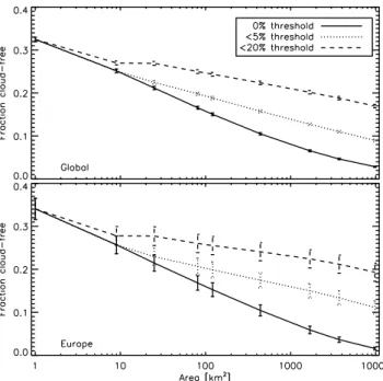
Figure1shows the fraction of cloud-free observations as a function of the area of the

10

simulated footprint. The first panel is averaged globally between 70◦ North and South, excluding the polar regions. The second panel shows the same information but now averaged over the MODIS categories coast/desert/land over Europe (latitudes between 35oN and 73◦N, longitudes between 10◦W and 36◦E). Note the logarithmic area axis. Both panels show three different line-styles (solid, dotted and dashed) for footprints

15

designated 0%, 5% cloud fraction or less, and 20% cloud fraction or less, respectively. Rounding errors occur when observing 9 km2(3 km×3 km). In this case the number for 5% cloud fraction or less is identical to 0%, because the possible cloud fractions are 0, 0.11, 0.22, 0.33,. . . , etc, and the number for 20% or less is effectively for 11% or less.

Globally we see a decrease in the fraction of cloud-free observations as a function

20

of area from about one-third at 1 km×1 km to only 3% percent of all observations at 10 000 km2. The decrease is almost logarithmically linear up to synoptic scales of sev-eral hundred km2 from whereon a further increase in footprint size causes relatively less extra cloud flagging. The numbers above are using the strict cloudiness thresh-old of 0% , where a single cloudy 1 km×1 km MODIS observation within the footprint

25

causes a full footprint to be designated cloudy. By application of a less strict threshold 4473

(11)

ACPD

Full Screen / Esc

on cloudiness the fraction of cloud-free observations is increased and the decrease with area is less steep. For footprints with up to 5% and up to 20% cloudiness we find at 10 000 km2 useful fractions of 0.09 and 0.17, respectively. The latter numbers are roughly applicable to GOME-1 on ERS-1.

The lowest panel of Fig. 1 shows that there is, coincidently, little difference

be-5

tween the fraction of cloud-free observations globally and for the MODIS categories land/desert/coast over Europe. For possible future air quality applications for the Eu-ropean continent the fraction of cloud-free observations for, for example, an area of 100 km2 are for the three thresholds (0%, up to 5%, up to 20%), respectively, 0.16, 0.20, and 0.26. Numbers at 3200 km2, which are applicable to the GOME-2 instrument,

10

are significantly smaller and down to 4% for the 0% threshold. The standard deviations over Europe are larger than globally because of the larger seasonal variations. These are further detailed in the next section.

3.1.1 Seasonal variation

Figure 2 shows the same parameter as Fig. 1 (lower panel), but now differentiated

15

between seasons and using “up to 5%” as cloudiness threshold. For the seasonal averages the data for six days (two days per month) have been used: winter is denoted by DJF (December, January, February), spring by MAM (March, April, May), summer by JJA (June, July, August), and autumn by SON (September, October, November). The panel for the global average is not shown as on a global scale the differences between

20

seasons are almost non-present, mainly because the northern-hemisphere winter is averaged with the southern-hemisphere summer and in reverse. The European winter clearly has the largest amount of clouds of the seasons, spring and autumn less, and not differing much from each other. European summer is relatively the most cloudfree.

(12)

ACPD

Full Screen / Esc

3.1.2 North and South Europe

A further refinement of the fraction of cloud-free observations as a function of sensor resolution over Europe can be obtained by differencing not only between the seasons, but also between northern and southern Europe. Because of the rather different cloud climatology significant differences in cloudiness are expected. For this purpose

north-5

ern Europe has been defined between 46◦N–58◦N and 10◦W–36◦E and southern Europe between 35◦N–46◦N and 10◦W–36◦E. Figure 3 shows that indeed the frac-tion of cloud-free observafrac-tions over southern Europe is typically twice the fracfrac-tion of cloud-free observations over northern Europe. The summer and autumn over southern Europe give a fraction of cloud-free observations of up to 0.70 and 0.53, respectively,

10

at 1 km×1 km, and 0.40 and 0.28 at 10 000 km2. The slopes as a function of sensor resolution (area) are rather similar. The standard deviations in the figure show that the daily variations within a season are quite large. Nevertheless, the differences be-tween the seasons are even larger. The geographical dependence of the results is further emphasized by Fig. 4. This figure illustrates the relative reduction in cloudy

15

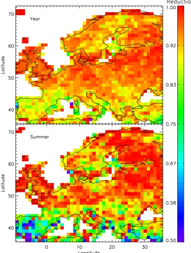
observations when sensor resolution would be increased from 3200 km2(applicable to GOME-2 on MetOp) to 100 km2. The upper panel shows the relative reduction in cloudy scenes for the summer season, the lower panel shows the yearly averages. Red col-ors indicate small relative reductions, green and blue significant relative reductions. Clearly the reductions are largest over southern Europe. While the relative reduction in

20

cloud-fractions seems minor, the increase of cloud-free observations due to improving sensor resolution may in fact be quite larger. A better way to quantify the impact of sen-sor resolution on fraction of cloud-free observations – particularly in persistently cloudy situations – is to calculate a relative gain factor. The relative gain factor is defined as the fraction of cloud-free observations for a sensor resolution of 100 km2divided by the

25

same value for a sensor resolution of 3200 km2and is a useful additional parameter as the gain factor puts more weight on extra cloud-free observations in particularly cloudy areas. For example, an area with a yearly cloud cover of 90% at 3200 km2resolution

(13)

ACPD

Full Screen / Esc

and 80% at 1000 km2resolution, has only a relative cloud reduction of 89%, while the relative gain cloud-free factor is 200%. The drawback for the gain factor is that infinite numbers may occur in grid cells where cloud-free observations are completely absent. Therefore no meaningful geographic images, such as Fig.4, can be easily shown. In-stead, our interest in future Earth observation of air quality, we compare gain factors

5

with reduction factors for a number of major cities in Europe, see Table1. The cities are ordered as a function of their fraction of cloud-free observations . In summer 2004 the cities with the largest fraction of cloud-free observations are Madrid (0.66) and Athens (0.63). The gain factors for these cities are 1.20 and 1.36, respectively. This implies that the number of cloud free observations over these cities would increase by about

10

30% using a footprint of 100 km2 instead of 3200 km2 (applicable to GOME-2). The smallest fraction of cloud-free observations at 3200 km2resolution is found for London (0.05). The number of cloud-free observations in the summer over London increases by more than a factor four for the high spatial resolution (100 km2) case. Tabel 1 also presents the annual numbers for the different cities.

15

3.1.3 Northern South America

Air pollution is a global phenomenon. For example, in the tropics the impact of human activities on atmospheric composition is increasing rapidly. Satellite observations of trace gases down to the boundary layer in tropical areas that are mostly poorly sampled by groundbased measurements would offer a wealth of information for studies on global

20

change. In order to examine the advantage of improved sensor resolution for a cloudy region outside Europe, we decided to investigate the area of the Amazon rain forest. The question is if an increase of sensor resolution would also give an increase of cloud free observations for this region. To answer this question we studied cloud statistics based on MODIS data for 2004 over South-America and in more particular the Amazon

25

area. For the analysis the observations are split into two seasons (wet and dry). Our division in seasons is based on examination of the MODIS cloud statistics for 2004.

(14)

ACPD

Full Screen / Esc

First we arbitrarily broke up the land-mass of South-America into three regions: South (5◦S–10◦S), Equator (5◦S–5◦N), and North (5◦N–15◦N) as indicated by solid curves in Fig.5. Note that the northern region contains only a small area of landmass. Observations over the Andes (indicated in red in the right-hand side panel) have been removed in order to prevent orography effects. As the centre of convection moves in

5

latitudinal direction during the year, the three different regions experience wet and dry seasons during different periods in the year (Hastenrath,1997).

Figure5shows the yearly variation of fraction of cloud-free observations over South-America for 2004. The same plot is shown twice in order to better show the annual cycle. For the purpose of our study the period during which a region has a low fraction

10

of cloud-free observations will be referred to as the “wet season”. Similarly, the period during which the fraction of cloud-free observations is high will be referred to as the “dry season”. In this manner the dry season is defined to last for the northern region from January to March and August to October, for the Equator regions from June till November and for the southern region from May till October. It is acknowledged that

15

the division in (multiple) dry and wet seasons could have been made somewhat more thoroughly. However, the main driver for the present study is to obtain a subtantial difference in cloud statistics between the seasons. Our division is roughly in line with the division in seasons as reported in the literature (Hastenrath,1997).

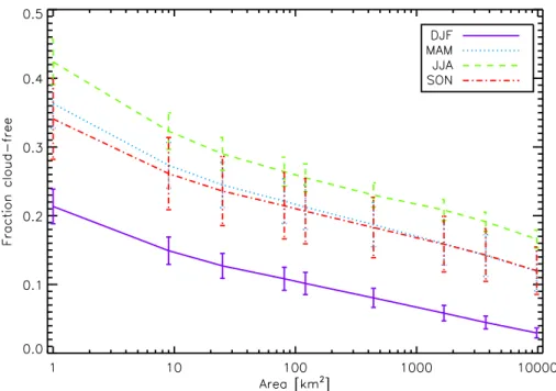
Figure6shows the fraction of cloud-free observations over land and averaged over

20

the wet and dry seasons for the different regions. Again observations over the Andes have been removed. As desired the wet seasons show a much lower fraction of cloud-free observations than the dry seasons, most clearly in the southern region. Northern South-America is showing more seasonal variation than Europe: the wet season is comparable in cloudiness to the European winter (Fig.1), while the dry season

com-25

pares to the summer in southern Europe (Fig.2). This is well in line withAsner(2001) who investigated the seasonal variation in cloudiness over the Brazilian Amazon using Landsat images (∼30 m resolution) of 185 km×185 km.

Figure7is similar to Fig.4for Europe. The geographical distribution of the reduction 4477

(15)

ACPD

Full Screen / Esc

in cloudy scenes is presented for an increase in sensor resolution from 3200 km2 to 100 km2. The upper and lower panel show the reductions for the dry and wet season, respectively, for each of the three defined regions. The reduction in cloudy scenes in the dry season is substantial, while reductions in the wet season are only marginal. However, this should be compared with the results in terms of a gain factor, again

5

defined as the number of cloud-free observations in a 1 km×1 km grid cell for a sensor resolution of 100 km2divided by the same value for a sensor resolution of 3200 km2. In Table2the absolute fraction of cloud-free observations as well as their associated gain factors are presented as a function of 5-degrees latitude bands in the region. Values are averages for a band between longitudes of 57◦W and 63◦W. The gain factors show

10

that also in the wet seasons significant more cloud free observations are obtained with increased resolution. While the fraction of cloud-free observations stays small, the number of cloud free observations is calculated to exceed 5 times the number of lower resolution observations in the [−10, −5] latitude band. We conclude that above tropical regions, and even in the wet season, a high sensor resolution will improve sensitivity

15

to trace gases in the lower troposphere by looking between clouds.

4 Discussion

It is interesting to compare our results with earlier works, both in absolute number of cloud-free observations and in its dependence on footprint area. For example, in the ACECHEM study (2001) global average statistics for a single day (4 July 1996) was

de-20

rived from 1 km×1 km ATSR-2 images. Our fraction of cloud-free observations based on 24 days of global data from MODIS TERRA are somewhat lower, yet the difference decreases when comparing only the fraction of cloud-free observations for July 2004 (22% vs 14% at 1600 km2, respectively) while the change with sensor resolution is al-most identical. Therefore, the MODIS cloud screening procedures that is applied here

25

is likely more stringent and makes use of the full suite of MODIS observations at di ffer-ent wavelengths, as MODIS has more channels than ATSR-2. As the ACECHEM study

(16)

ACPD

Full Screen / Esc

analysed only a single day, temporal variation might also confuse direct comparison. In another study byTjemkes et al.(2003), per season one week of cloud mask data from a geosationary platform was studied. They found that the fraction of cloud-free ob-servations values are twice as large as in our study, yet with similar change with sensor resolution. Yet their study did not try to establish an absolute reference. The employed

5

cloud-mask might underestimate the number of clouds as the cloud-detection algorithm was designed for SEVIRI on Meteosat Second Generation (Meteosat-8), but applied on its predecessor, MVIRI on Meteosat-7. MVIRI contains only three observation chan-nels. The MODIS cloud mask algorithm used in our study is more advanced because it can make use of much more spectral channels, see the specifications in Sect.2.2.

10

Also the initial cloudmask of MODIS is of higher sensitivity due to MODIS better reso-lution (1 km×1 km) compared to MVIRI (7.5 km×7.5 km). All cloud detection methods sometimes overlook a cloud that covers only a very small area of the total footprint, as such very small clouds might be missed by MVIRI but not by MODIS. Finally MODIS is cloud conservative, as shown byLi et al. (2005), which is a desired property of cloud

15

mask employed to remove cloudy observations.

Our study agrees with earlier studies which analyzed cloud fractions for a single resolution, such asBr ´eon et al. (2005), who found at 7 km along-track resolution us-ing GLAS observations around 30% “almost clear sky” (aerosols and clouds τ<0.2) over Europe and ∼32% globally during autumn 2003. The corresponding numbers

20

from our study are 27% and 28%, respectively, which correspond very well given the uncertainties. Meerkotter et al. (2004) found, using 14-years of AVHRR and SYNOP observations, and at 1 km×1 km resolution, for northern Europe a yearly fraction of cloud-free observations around 35% and for southern Europe around 55%. The corre-sponding numbers from our study are 27% and 50%, respectively, which correspond

25

very well given the larger uncertainties as they study smaller areas (individual coun-tries). As such they confirm the differences we found between northern and southern Europe. Using 7 km×5 km Meteosat observations spanning from August 1994 till July 1995 Massons et al.(1998) found an annual fraction of cloud-free observations over

(17)

ACPD

Full Screen / Esc

northern Europe between 10–40% and over southern Europe between 40–70%, which compares very will with our results of 27% and 50%, respectively.

This study was limited to data from one year, 2004, and within this year, we examined two days of MODIS data per month: the 1st (or 2nd) and 15th day. It is therefore unlikely that our data set covers the full temporal variation in cloudiness. For example,

5

we noted that on 15 April 2004 central Europe was relatively cloud free. However, we assume that the effect of imperfect temporal sampling will be smaller when we average over a large enough area, capturing enough spatial variation to compensate for the temporal variation. E.g., while central Europe was cloud-free, northern Europe was quite clouded. We did some tests (not shown here) which confirmed that the effects

10

of our limited temporal sampling does not affect the results when we look at averages over areas of a single (sub-)continent or larger. Numbers for smaller regions such as given in Table 2, and especially for cities such as given in Table 1 will suffer more from the limited sampling of our data set. One could certainly question their general representativeness. Nevertheless, we considered it worthwile to present some of our

15

results not only on continental scales.

We also analyzed MODIS/AQUA observations for the 15th of each month, search-ing for diurnal variation, as MODIS/TERRA has a local overpass time of 10:30 and MODIS/AQUA at 13:30. However we found very little difference within the uncertain-ties. From this we tend to conclude that the considered overpass times would be

20

equally adequate for missions focusing on air quality. It is noted that to study diurnal variation it would be preferably to employ a single instrument because the construc-tion of different instruments may introduce (technical) differences, even if of similar design. Also a larger time difference (e.g. between 10:30 and 16:00) would be needed for a proper study of diurnal variations. In this study we chose to analyse

observa-25

tions from MODIS/TERRA because MODIS/AQUA is missing a channel and because MODIS/TERRA is in descending orbit, similarly as GOME, SCIAMACHY, OMI, and GOME-2.

In this work we did not study the effect of cirrus clouds that are optically thin (optical 4480

(18)

ACPD

Full Screen / Esc

thickness <0.2) in the visible wavelength range but well observed in the infrared. Thin cirrus clouds can significantly influence retrievals of trace gas constituents. Cirrus clouds occur most frequently at higher altitudes (>10 km) and in the tropics and less often at lower altitudes (∼6 km) and at mid-latitudes. The MODIS cloud mask product gives information on the possible presence of optically thin clouds. Based hereon

5

we concluded that thin cirrus occur globally for less than 4% of all otherwise clear sky scenes. For Europe we find less than 2%. In a recent study by Breon et al. (2005) using Geoscience Laser Altimeter System (GLAS) observations (7 km along track resolution) it is shown that optical thin (<0.2) clouds occur for about 8% of the scenes in the tropics and also much less at mid-latitudes.

10

Finally, shadowing of clouds could have an impact on the determination of the frac-tion of cloud-free scenes. Based on our (limited) MODIS data-set we conclude that shadowing will impact on the number of cloud-free scenes by less than 4% globally, and less than 0.5% over Europe.

5 Conclusions

15

Recent satelliteborne trace gas column observations sensitive to the lower troposphere and planetary boundary layer show large potential for air quality applications (e.g. by constraining air quality analyses and forecasts) and for studies on human impact and global change (e.g. by surface emission inversions). Envisioned applications require footprints that are minimised for the effect of clouds. In this paper we have investigated

20

the potential to increase the fraction of cloud-free observations by an increase in sen-sor resolution. We have quantified the benefits globally and for two regions with very different cloud regimes: Europe and northern South America. We used the 1 km×1 km MODIS TERRA cloud mask for our calculations. We have also demonstrated that the relative gain in cloud-free observations as a function of sensor resolution is largest in

25

the less cloudy regions and seasons. However, it is anticipated that the foreseen ad-dition of only a few cloud-free observations (in absolute number) in persistently cloudy

(19)

ACPD

Full Screen / Esc

regions and seasons is also very important for the observation from space of the at-mospheric composition in the lower troposphere.

In our study we have quantified the “fraction of cloud-free observations” and the in-crease of cloud-free observations for higher sensor resolutions. Under the assumption of a preserved sampling rate (that is, e.g., related to revisit time and swath) a

dou-5

bling of sensor resolution would imply by definition a doubling of the absolute number of cloud-free observations over a certain area. This factor is typically larger than the change in cloud fraction and easy to quantify. Combined with the increase of useful cloud-free footprints this allows e.g., a future mission with 10 km×10 km footprint and similar swath to GOME-2 to statistically obtain as much cloud-free measurements over

10

Northwest Europe in less than a week as GOME-2 obtains in a full year.

Finally, the absolute number of cloud-free observations over a certain region can be increased by increasing the revisit time of the observations. This can be accom-plished in different ways. First, by using a wide swath. For example, the wide swath of OMI and MODIS yield global coverage in one day while GOME-1 on ERS-2 only

15

obtained global coverage in three days. An instrument could also be positioned on a geostationary platform or in low-inclination orbit instead of the more common polar or-bit. These configurations would in addition allow to observe diurnal variations in trace gas concentrations. The absolute number of cloud-free observations using these ge-ometries will not increase if the clouds persist over the whole day. A similar study as

20

presented here, but using cloud mask data from instruments on a geostationary plat-form is needed to quantify to what extend the number of cloud-free observations for certain regions would be increased by performing multiple observations per day. Diur-nal variation in cloudiness changes from day-to-day, depending on the weather, and is a function of geolocation and season.

25

Acknowledgements. We would like to thank J. de Laat for his comments. The MODIS data

used in this study were acquired as part of the NASA’s Earth Science Enterprise. The MODIS cloud mask algorithms were developed by the MODIS Science Teams. The MODIS cloud mask data were processed by the MODIS Adaptive Processing System (MODAPS) and Goddard

(20)

ACPD

Full Screen / Esc

Distributed Active Archive Center (DAAC), and are archived and distributed by the Goddard DAAC. The authors have obtained additional and more specialised statistics from the presented data, e.g., concerning different observation techniques or cloud thressholds. Those interested in using these additional cloud-statistics from the used dataset can contact the first author.

References

5

Ackerman, S. A., Strabala, K. I., Menzel, W. P., Frey, R. A., Moeller, C. C., Gumley, L. E., Baum, B., Wetzel-Seeman, S., and Zhang, H.: Discriminating clear sky from clouds with MODIS Algorithm Theoritical Basis Document (MOD35), Tech. Rep. ATBD-MOD-06, University of Wisconsin-Madison, 2002. 4469,4470

Asner, G.: Cloud cover in Landsat observations of the Brazilian Amazon, International Journal

10

of Remote Sensing, 22, 3855–3862, 2001. 4477

Boersma, K. F., Eskes, H. J., and Brinksma, E. J.: Error analysis for tropospheric NO₂retrieval from space, J. Geophys. Res.-Atmos., 109, D04 311–D04 322, 2004. 4468,4472

Bovensmann, H., Burrows, J. P., Buchwitz, M., Frerick, J., Noel, S., Rozanov, V. V., Chance, K. V., and Goede, A. P. H.: Sciamachy: Mission objectives and measurement modes, J.

15

Atmos. Sci., 56, 127–150, 1999. 4468

Br ´eon, F. M., O’Brien, D. M., and Spinhirne, J. D.: Scattering layer statistics from space borne GLAS observations, Geophys. Res. Lett., 32, 22 802, doi:10.1029/2005GL023825, 2005.

4479

Burrows, J. P., Dehn, A., Deters, B., Himmelmann, S., Richter, A., Voigt, S., and Orphal, J.:

At-20

mospheric remote-sensing reference data from GOME: 2, Temperature-dependent absorp-tion cross secabsorp-tions of O₃in the 231–794 nm range, J. Quant. Spectrosc. Radiat. Transfer, 61, 509–517, 1999. 4467

ESA: The five candidate earth explorer core missions, Reports for Assessment, ACECHEM, Tech. rep., ESA, 2001.

25

Gloudemans, A. M. S., Schrijver, H., Kleipool, Q., van den Broek, M. M. P., Straume, A. G., Lichtenberg, G., van Hees, R. M., Aben, I., and Meirink, J. F.: The impact of SCIAMACHY near-infrared instrument calibration on CH4 and CO total columns, Atmos. Chem. Phys., 5, 1733–1770, 2005. 4472

Harshvardhan, B. A., Wielicki, B. A., and Ginger, K. M.: The Interpretation of Remotely Sensed

30

(21)

ACPD

Full Screen / Esc

Cloud Properties from a Model Parameterization Perspective, J. Clim., 7, 1987–1998, 1994.

4469

Hastenrath, S.: Annual cycle of upper air circulation and convective activity over the tropical Americas, J. Geophys. Res., 102, 4267–4274, 1997. 4477

Kelder, H., van Weele, M., Bovensmann, H., Goede, A., Kerridge, B., Mager, R., Monks, P.,

5

Reburn, W., Remedios, J., and Sassier, H.: Operational Atmospheric Chemistry Monitoring Missions: CAPACITY, final report, ESA contract no. 17237/03/NL/GS, Tech. rep., ESA, 2005.

4468

Leue, C., Wenig, M., Wagner, T., Klimm, O., Platt, U., and J ¨ahne, B.: Quantitative analysis of NO_x emissions from Global Ozone Monitoring Experiment satellite image sequences, J.

10

Geophys. Res., 106, 5493–5506, 2001. 4468

Levelt, P. F., van den Oord, B., Hilsenrath, E., Leppelmeier, G. W., Bhartia, P. K., Malkki, A., Kelder, H., van der A, R. J., Brinksma, E. J., van Oss, R., Veefkind, P., van Weele, M., and Noordhoek, R.: Science Objectives of EOS-Aura’s Ozone Monitoring Instrument (OMI), in: Proc. Quad. Ozone Symposium, pp. 127–128, 2000. 4468

15

Li, Z., Crib, M., Chang, F.-L., Trishchenko, A., and Luo, Y.: Evaluating MODIS Cloud Detection Algorithm Using Whole-Sky Imager Cloud Cover Data at the Three ARM Sites, in: Fifteenth ARM Science Team Meeting Proceedings, Daytona Beach, Florida, 2005. 4479

Martin, R. V., Parrish, D. D., Ryerson, T. B., Nicks, D. K., Chance, K., Kurosu, T. P., Jacob, D. J., Sturges, E. D., Fried, A., and Wert, B. P.: Evaluation of GOME satellite measurements of

20

tropospheric NO₂and HCHO using regional data from aircraft campaigns in the southeastern United States, J. Geophys. Res., 109, D24307, doi:10.1029/2004JD004869, 2004. 4468

Massons, J., Domingo, D., and Lorente, J.: Seasonal cycle of cloud cover analyzed using Meteosat images, Ann. Geophys., 16, 331–341, 1998. 4479

Meirink, J. F., Eskes, H. J., and Goede, A. P. H.: Sensitivity analysis of methane emissions

25

derived from SCIAMACHY observations through inverse modelling, Atmos. Chem. Phys., 5, 9405–9445, 2005. 4467,4472

Richter, A. and Burrows, J. P.: Tropospheric NO₂from GOME measurements, Adv, Space Res., 29, 1673–1683, 2002. 4468

Richter, A., Burrows, J. P., Nusz, H., Granier, C., and Niemeier, U.: Increase in tropospheric

30

nitrogen dioxide over China observed from space, Nature, 437, 129–132, 2005. 4468

Tjemkes, S., Lutz, H., Duff, C., Stuhlmann, R., and McNally, A.: Detection of cloud-free areas as a function of Sensor Resolution and Time Sampling, Technical Memorandum No. 10,

(22)

ACPD

Full Screen / Esc

2003. 4469,4479

Wielicki, B. A. and Parker, L.: On the determination of cloud cover from satellite sensors: The effect of sensor spatial resolution, J. Geophys. Res., 97, 12 799–12 823, 1992. 4469

(23)

ACPD

Full Screen / Esc

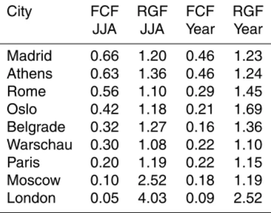
Table 1. Absolute fraction of cloud-free observations (FCF) at 100 km2 resolution and relative gain factor (RGF) between footprints of 100 km2 and 3200 km2 averaged over the summer of 2004 and for the full year of 2004. Threshold: up to 5% cloudiness.

City FCF RGF FCF RGF JJA JJA Year Year Madrid 0.66 1.20 0.46 1.23 Athens 0.63 1.36 0.46 1.24 Rome 0.56 1.10 0.29 1.45 Oslo 0.42 1.18 0.21 1.69 Belgrade 0.32 1.27 0.16 1.36 Warschau 0.30 1.08 0.22 1.10 Paris 0.20 1.19 0.22 1.15 Moscow 0.10 2.52 0.18 1.19 London 0.05 4.03 0.09 2.52 4486

(24)

ACPD

Full Screen / Esc

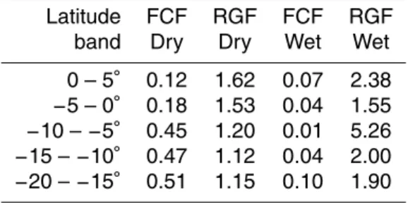
Table 2. Absolute fraction of cloud-free observations (FCF) and relative gain factor (RGF)

be-tween footprints of 100 km2and 3200 km2for wet and dry season over South America averaged between −63 and −57 E longitude for different indicated latitude bands. Threshold: up to 5% cloudiness.

Latitude FCF RGF FCF RGF band Dry Dry Wet Wet 0 – 5◦ 0.12 1.62 0.07 2.38 −5 – 0◦ 0.18 1.53 0.04 1.55 −10 – −5◦ 0.45 1.20 0.01 5.26 −15 – −10◦ 0.47 1.12 0.04 2.00 −20 – −15◦ 0.51 1.15 0.10 1.90 4487

(25)

ACPD

Full Screen / Esc

Fig. 1. The fraction of cloud-free observations as a function of sensor resolution (footprint area),

as determined from 1 km×1 km resolution MODIS TERRA (local overpass time 10:30 UT) cloud mask (MOD35) observations. For each month in 2004 two days (either the 1st or 2nd and the 15th) are analyzed and statistics determined. Different line-styles indicate different thresholds on cloudiness: 0% indicates that not a single MODIS cloud of 1 km×1 km was allowed to be present in the observed area. The data for the 5% and 20% thresholds includes the areas that were containing clouds up to 5% and 20%, respectively, of the total area observed. Also indicated are the standard deviations on the average derived from the temporal variation during the whole year (based on 24 days). Top panel: globally averaged between latitudes of 70◦S and 70◦N. Bottom panel: the same plot but averaged over Europe (latitude range 35◦N–73◦N; longitude range 10◦W–36◦E) for MODIS categories land, coast, and desert. Coincidently, these cloud-free fractions over Europe are very similar to the global averaged fractions in the upper panel that also include the oceans.

(26)

ACPD

Full Screen / Esc

Fig. 2. Similar as Fig.1, yet now only for the MODIS categories land/desert and coast, over Eu-rope, and with a threshold of up to 5% cloudiness. Different colors indicate averaging over dif-ferent seasons: winter: December, January, February (DJF); spring: March, April, May (MAM); summer: JJA (June, July, August); autumn: September, October, November (SON). Also in-dicated are the standard deviations on the average derived from the temporal variation during the season. Six days of global MODIS observations for the year 2004 have been analysed per season.

(27)

ACPD

Full Screen / Esc

Fig. 3. Similar as Fig.1(lower panel), with a threshold of up to 5% cloudiness, yet now splitted between the land masses of northern (dashed curves) and southern (solid curves) Europe. Indicated are also 1-sigma errors-bars derived from the temporal variation during the season. The error-bars from the North Europe observations are shifted slightly in area for clarity.

(28)

ACPD

Full Screen / Esc

Fig. 4. Relative reduction in clouded observations (up to 5% cloudiness thresshold) over

Eu-rope, when increasing sensor resolution from 3200 km2 to 100 km2. The upper panel shows the reductions averaged for the summer (JJA), the lower panel averaged over the whole year.

(29)

ACPD

Full Screen / Esc

Fig. 5. Yearly variation in 2004 of fraction of cloud-free observations with a threshold up to 5%

cloudiness (FCF) over northern South-America and surrounding waters for different 1◦

latitude bands. The plot is presented twice, in order to better show the cyclic yearly variation. On the right side an image of South-America is given (contracted in longitude) with the scenes over the Andes that have been left out, and for visual reference to the latitudes. The highest cloud fractions (in blue) move rather slow from South to North during the year and then quickly from North to South in November/December.

(30)

ACPD

Full Screen / Esc

Fig. 6. Similar as Fig.1, but now over northern Southern America. The fraction of cloud-free observations is shown for different sub-regions (blue, North [5◦N–20◦N], Equator [5◦S–5◦N] and South [20◦S–5◦S]) and seasons (solid curves: dry season, dashed curves: wet season). The area covered by the Andes has been removed. Indicated are also 1-sigma errors-bars derived from temporal variation during seasons.

(31)

ACPD

Full Screen / Esc

Fig. 7. Similar as Fig.4, but now showing the relative reduction in clouded observations during the dry (upper panel) and wet (lower panel) season over the northern South America.