HAL Id: hal-00318428
https://hal.archives-ouvertes.fr/hal-00318428
Submitted on 2 Jan 2008
HAL is a multi-disciplinary open access
archive for the deposit and dissemination of
sci-entific research documents, whether they are
pub-lished or not. The documents may come from
teaching and research institutions in France or
abroad, or from public or private research centers.
L’archive ouverte pluridisciplinaire HAL, est
destinée au dépôt et à la diffusion de documents
scientifiques de niveau recherche, publiés ou non,
émanant des établissements d’enseignement et de
recherche français ou étrangers, des laboratoires
publics ou privés.
Comparison of magnetic field observations of an average
magnetic cloud with a simple force free model: the
importance of field compression and expansion
R. P. Lepping, T. W. Narock, H. Chen
To cite this version:
R. P. Lepping, T. W. Narock, H. Chen. Comparison of magnetic field observations of an average
magnetic cloud with a simple force free model: the importance of field compression and expansion.
Annales Geophysicae, European Geosciences Union, 2008, 25 (12), pp.2641-2648. �hal-00318428�
www.ann-geophys.net/25/2641/2007/ © European Geosciences Union 2007
Annales
Geophysicae
Comparison of magnetic field observations of an average magnetic
cloud with a simple force free model: the importance of field
compression and expansion
R. P. Lepping1, T. W. Narock1,2, and H. Chen3
1NASA, Goddard Space Flight Center, Heliophysics Science Division, Greenbelt, MD 20771, USA 2Goddard Earth and Science Technology Center, University of Maryland, Baltimore County, MD, USA 3River Hill High School, Clarksville MD 21029, USA
Received: 1 June 2007 – Revised: 6 November 2007 – Accepted: 14 November 2007 – Published: 2 January 2008
Abstract. We investigate the ability of the cylindrically symmetric force-free magnetic cloud (MC) fitting model of Lepping et al. (1990) to faithfully reproduce actual magnetic field observations by examining two quantities: (1) a difference angle, called β, i.e., the angle between the direction of the observed magnetic field (Bobs) and
the derived force free model field (Bmod) and (2) the
dif-ference in magnitudes between the observed and modeled
fields, i.e., 1B(=|Bobs|−|Bmod|), and a normalized 1B (i.e.,
1B/<B>) is also examined, all for a judiciously chosen set of 50 WIND interplanetary MCs, based on quality consid-erations. These three quantities are developed as a percent of MC duration and averaged over this set of MCs to obtain average profiles. It is found that, although <1B> and its normalize version are significantly enhanced (from a broad central average value) early in an average MC (and to a lesser extent also late in the MC), the angle <β> is small (less than 8◦) and approximately constant all throughout the MC. The field intensity enhancements are due mainly to interaction of the MC with the surrounding solar wind plasma causing field
compression at front and rear. For example, for a typical MC,
1B/<B> is: 0.21±0.27 very early in the MC, −0.11±0.10 at the center (and −0.085±0.12 averaged over the full “cen-tral region,” i.e., for 30% to 80% of duration), and 0.05±0.29 very late in the MC, showing a double sign change as we travel from front to center to back, in the MC. When individ-ual MCs are examined we find that over 80% of them possess field enhancements within several to many hours of the front boundary, but only about 30% show such enhancements at their rear portions. The enhancement of the MC’s front field is also due to MC expansion, but this is usually a lesser effect compared to compression. It is expected that this compres-sion is manifested as significant distortion to the MC’s cross-section from the ideal circle, first suggested by Crooker et
Correspondence to: R. P. Lepping
(ronald.p.lepping@nasa.gov)
al. (1990), into a more elliptical/oval shape, as some global MC studies seem to confirm (e.g., Riley and Crooker, 2004) and apparently also as confirmed for local studies of MCs (e.g., Hidalgo et al., 2002; Nieves-Chinchilla et al., 2005).
Keywords. Solar physics, astrophysics and astronomy
(Flares and mass ejections, Magnetic fields) – Space plasma physics (experimental and mathematical techniques)
1 Introduction
We are concerned here with evaluating the capability of the force-free cylindrically symmetric (and so-called con-stant alpha) magnetic cloud (MC) fitting model of Lepping et al. (1990) to reproduce average input data (average mag-netic field vector observations), for relatively good quality MCs, as defined below. This model is based on MC prop-erties earlier discussed by Burlaga et al. (1981), Goldstein (1983), and Burlaga (1988). A MC was defined empiri-cally by L. Burlaga and coworkers as a (usually large) in-terplanetary structure having enhanced field magnitude, a relatively smooth change in field direction as the space-craft passes through the MC, and lower proton temperature (and proton beta) than the surrounding solar wind (see, e.g., Burlaga, 1995). In particular, we analyze here the Lepping et al. (1990) model’s average ability to provide separately field directions and field magnitudes that are consistent with ob-servations using a large number of WIND MCs. It is well know that this model is relatively good at reproducing the actual direction of the field for most events (and it generally provides good estimates of most of the model fit parameters, especially axial attitude, Lepping et al., 2003a, 2004), but its ability to capture the field magnitude profile across the MC is almost always poor. This is believed to be mainly due to the two oversimplifying assumptions that were employed in the model: (1) circular cross-section and (2) static nature of
2642 R. P. Lepping et al.: Comparison of magnetic field observations the MC (i.e., non-expanding). So we ask, “How faithful, on
average, is the field directional-profile reproduction, and how poor is the field magnitude-profile reproduction by the model – and where is it poorest”?
Lepping et al. (2003a, also see 2004) took a different approach in studying the Lepping et al. (1990) MC fitting model’s ability to reproduce observations by showing how the “fluctuation level” of the field within a MC can propagate to the seven MC fit-parameter error estimates; the higher the fluctuation level the higher the parameter uncertainty. (Er-rors due to choosing incorrect boundary times were not con-sidered. ) Other independent variables affecting uncertainty, besides the fluctuation level, were the closest approach dis-tance and the size of the oblique angle that the spacecraft’s path makes with the MC’s axis. Such error estimates for the MC fit-parameters hold for the given MC as a whole. The study here is concerned with finding quantitatively how field observations typically deviate from the MC model field, as a
function of percent travel through the average MC, i.e., as a function of space, and with any implications.
2 Analysis and results: field direction
We start by defining a difference angle (called β), which is that angle between the direction of the observed magnetic field within a MC and that direction of the field derived by the Lepping et al. (1990) MC fitting model (assumed for the same instant front and rear. For examplind it convenient to present β as a percent of MC duration through the MC, so we can superimpose many MCs of various actual sizes to find an “average” case. We, in fact, do this using a large num-ber of good quality WIND MCs; quality (QO)is defined in
Lepping et al. (2006). That is, only MCs of QO of 1 or 2
are used, i.e., those of QO=3, quantitatively determined poor
cases, are ignored in forming the average β. These QO=1,2
cases comprise 50 MCs out of an original 82, for the inter-val from WIND launch until August 2003. We determined that it is very important to smooth the field observations, through filtering, before any difference quantity is formed; this smoothing is done with three trial running averages to be explained below. We justify this field-smoothing on the basis of our desire to judge the MC parameter fit-model’s ability to track the major component of the observed MC, i.e., we do not wish to follow all the little wiggles in the field that are usually due to waves and/or discontinuities superimposed on the MC’s field and which are not considered part of the MC (see, e.g., Narock and Lepping, 2007).
First, we will discuss how average β (<β>) is derived. We start by “low pass filtering” the one minute averages of the magnetic field within each MC of the 50 cases of interest with a running average filter, in order to smooth
the observations, as mentioned above. [The 1 min averages
were derived by averaging WIND/MFI measurements that were made at the standard sample rate of ≈11 vector
sam-ples/s (usually) done in component form.] This is done for three trial smoothing-intervals (denoted 1T ) of 15, 61, and 242 min; see Lepping et al. (2007) for an identical analysis using five smoothing intervals. (No interval lengths longer than 242 min were attempted.) After this, the resulting MCs are still in one minute average form. We then divide the dura-tion of the MC into 100 evenly spaced buckets, so that each bucket represents one percent of the duration of that MC. In this way we can superimpose the 50 MCs regardless of the actual differences in their durations. [Since we limit the study to only the better quality MCs, QO of 1 and 2 cases
(see Lepping et al., 2006), we are less likely to badly distort the results by those extreme cases of very distant passages where only a very small outer segment of the MC would be contributing to the average. Actually, only six cases of the 50 had closest approaches greater than 66% of the radius.] How-ever, by employing percent-duration means that the origi-nal 1 min averages must be averaged in each MC separately to whatever interval is necessary to create the 100 averages across the MC. Typically such an average is about 13 min, since the average MC-duration was 21.6 h for these 50 MCs (e.g., see Lepping et al., 2006). The model field, however, was based on the discrete averages (which could have been any one of 1T′=15, 30, or 60 min depending on the duration of the MC); the results are shown in Table 2 of the Website: http://lepmfi.gsfc.nasa.gov/mfi/mag cloud S1.html
It is obvious that there was no need for “model-curve smoothing”, because the resulting model-field is already rep-resented as a smoothed vector field, in time, from the Lep-ping et al. (1990) fitting procedure itself. We pick 100 evenly spaced vectors from the model-field for each MC and, along with the 100 matched observed fields, as described above, we find 100 β’s using
β =cos−1(Bobs·Bmod/(|Bobs||Bmod|)), (1)
at each of the 100 points for each MC, where Bobs is the
observed field and Bmodis the model field.
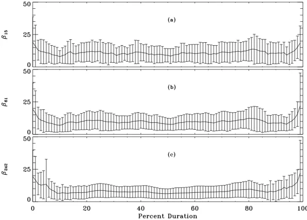
After these operations, the 100 points (β’s) of each of the 50 MCs are averaged, and these averages and their associ-ated standard deviations (σ , i.e., the RMSs) are retained; the results are shown in Fig. 1, where the curves are labeled (a) to (c), according to the scheme of Table 1. The central curves are the averages of β, and the length (top-to-bottom) of the vertical bar at each point represent twice the sigma for that point. It is obvious that set (a) is more jagged generally, has higher sigmas, and its average is higher than those of all the other curves. But what all three average curves have in com-mon is an approximate constancy across the full 100% du-ration, except for some boundary influences. As might be expected, set (c), where the smoothing interval is largest at 242 min, has the broadest boundary influence, but this set is the smoothest, has the lowest overall average value (of 7.6◦, if the average is taken between 10% and 90% duration), and is the most constant between 10% and 90%-duration. (The
Table 1. The final averages and sigmas for β*, 1B+, and 1B/<B>+for three smoothing interval lengths.
Case Interval length <<β>> <σβ> <<1B>> <σ1B> <<1B/<B>>> <σ1B/<B>>
1T(minutes) (Deg) (Deg) (nT) (nT)
(a) 15 10.8 7.3 −0.88 2.04 −0.060 0.13
(b) 61 9.7 6.4 −0.93 2.06 −0.064 0.14
(c) 242 7.6 4.9 −1.18 1.90 −0.085 0.12
* Average and sigma derived over the interval of 10% to 90% of duration for β.
+Average and sigma derived over the interval of 30% to 80% of duration for 1B and 1B/<B>.
Table 2. Comparisons of <<1B>> and <<1B/<B>>> within the Average Magnetic Cloud for the 1T =242 Minute Case.
Quantity Considered: <<1B>> <σ1B> <<1B/<B>>> <σ1B/<B>>
(nT) (nT)
Very early in the MC 3.5 4.5 0.21 0.27
At the Center −1.6 1.8 −0.11 0.10
For the full “central region* −1.2 1.9 −0.085 0.12 Very late in the MC 0.60 3.4 0.05 0.29
* This region refers to 30% to 80% of duration within the average MC, the “average-middle region” for study of field magnitude differences.
fact that duration of the enhanced boundary effect for β de-pends on the filter-length, being almost negligible for the 15 min case, clearly indicates that these small variations in
β near the boundaries are due to filtering, are not real, and can be ignored.) The left side of Table 1 shows the averages and sigmas for β (i.e., <<β>>, <σβ>)derived from each
of the three curves, over the interval of 10% to 90% to avoid boundary concerns. The 242 min average curve (c) gives the smallest <<β>> and <σβ>(4.9◦), as mentioned above,
and we will consider it to give the best estimate of <<β>>. Further we will assume that <β> is approximately constant all across the average MC, because of the argument above concerning the 15 min case. The main point here is that for a fixed 1T , <β> and σβ are almost constant and small all
across the average MC, including the regions close to the
boundary.
3 Analysis and results: field magnitude
We now examine the difference between the
magni-tudes of the observed (obs) and modeled (mod) fields
(1B=|Bobs|−|Bmod|), for the same time intervals as were
studied for β, and also as a percent of MC duration through the MC, again for only QO=1 and 2 cases. These field
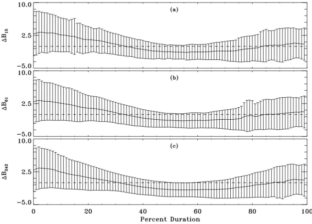
inten-sity differences are processed in the same manner as β with respect to smoothing and averaging, and the results are given in Fig. 2, which shows 1B vs. %-duration for the same three
1Ts 15 to 242 min [i.e., (a) to (c)]. But we see that 1B has very different characteristics compared to β. Whereas the three average β-curves of Fig. 1 are approximately
sym-metric around 50% (and almost constant vs. %-duration), the three 1B-curves are clearly not constant anywhere, not sym-metric, and have roughly a broad “U” shape. The values of
<1B>at the beginning of each panel are relatively high and the associated sigmas are also high. The middle columns of Table 1 show the averages and sigmas for 1B (<<1B>>,
<σ1B>)derived from each of the three curves in Fig. 2 over
the interval of 30% to 80% of duration, where the curves are near minimum, mostly negative, and deviate only slightly from being flat. [In a report by Lepping et al. (2007) where
|1B| is examined (as well as 1B itself), it is seen that in the region from 30% to 80% of duration of the average MC the ordinate value is relatively steady much like β is in the region of 10% and 90%-duration; see Figs. 7, 8 and 9 of that report. Hence, the region between 30% and 80% of dura-tion is separated from the two “boundary” regions (<30% and >80%), as in Figs. 2 and 3 and in Table 1 here. But
|1B| itself will not be discussed here.] As Table 1 shows, the changes in these quantities vs. 1T -length (a to c) is also very regular, with the 1T =242 min (c) giving the smallest average sigma of <σ1B>of 1.9 nT, yielding a <<1B>>
of −1.2 nT. However, it is interesting that <<1B>> and
<σ1B>are almost independent of the value of 1T ,
espe-cially so for <σ1B>. The 1B results are clearly less
sensi-tive to 1T than the β results.
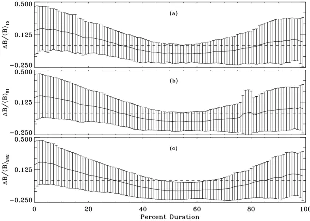
Since the average fields across these 50 MCs cover a very broad range (from 5 nT to 31 nT), and with model-estimated axial values covering the range of 9 nT to 47 nT (e.g., see Lepping et al., 2006), it is often reasonable and informative to normalize each MC’s 1B by its average <B>. Then all
2644 R. P. Lepping et al.: Comparison of magnetic field observations
Fig. 1. Family of plots of β vs. %-duration for three 1T s (from top to bottom: 15, 61, and 242 min, as shown by the subscripts on the β’s
on the left). The central curves are the averages over the 50 MCs, and the lengths (top-to-bottom) of the vertical bars at the points represent twice their sigmas.
of those in the full set of 50 MCs are on the same footing when they are superimposed, when finding the overall av-erage MC. In fact, superimposing such a normalized quan-tity probably makes more sense than simply superimpos-ing 1B itself. Therefore, in Fig. 3 we show the normal-ized 1B (i.e., 1B/<B>) vs. %-duration for the same three
1Ts. The right side of Table 1 shows <<1B/<B>>> and
<σ1B/B>derived from each of the three curves in Fig. 3,
again over the region of 30% to 80% of duration, and where again the regions near the boundaries are ignored. It is inter-esting that in this “middle” region the model gives a slightly
higher estimate than the observations, (i.e., << 1B>> and
<< 1B/<B>>> are both negative), as Table 1 shows, unlike the early or later regions. Table 1 also shows that, for this central region, there is little variation of either
<< 1B/<B>>> or its sigma as 1T -length is changed over 15 to 242 min, as was true for <1B> itself, with how-ever <σ1B/B>being the smallest (0.12) for 1T of 242 min,
where << 1B/<B>>>=−0.085. We also notice that for
1T of 15 min |<<1B/<B>>>| is the smallest, 0.060. The boundary regions obviously would show larger values of both |1B| and its <σ1B>.
As Figs. 2 an 3 show the model does not do so well in estimating field intensity closer to the boundaries in terms of either <1B> or <1B/<B>>. In particular, for a “typical,” good MC (i.e., for QO=1,2 quality cases where the
smooth-ing average is 242 min), 1B is about 3.5 nT±4.5 nT very early in the MC, −1.6 nT±1.8 nT in the middle (which for the full region of 30% to 80% of duration is −1.2 nT±1.9 nT; see Table 1), and 0.60 nT±3.4 nT at the end. We consider the 242 min case here, because it gives the lowest <σ1B>
(=1.9 nT) in that middle range of durations, as Table 1 shows. See Table 2 for a comparison of 1B (and σ1B) at
vari-ous key locations in the average MC. Similarly for such a typical MC, 1B/<B> is 0.21±0.27 very early in the MC, about −0.11±0.10 at the center (and for the full region of 30% to 80% of duration is −0.085±0.12; see Table 1), and 0.05±0.29 late in the MC, as Fig. 3 and Table 2 show. So the quantities |<1B>| and |<1B/<B>>| very near the front are larger than the average-middle region by factors of 2.2 and 1.6, respectively. We also see that there is a sign change of <1B> (and <1B/<B>>) from either of the near-boundary values (being positive) to the central val-ues, which are negative. Obviously any individual MC can have difference-values that are quite at variance from these
Fig. 2. Family of plots of 1B (=Bobs−Bmod)vs. %-duration for three 1T s (from top to bottom as in Fig. 1a, b, c, as shown by the subscripts
on the 1Bs on the left). The central curves are the actual averages over the 50 MCs, and the lengths (top-to-bottom) of the vertical bars at the points represent twice their sigmas. The dashed line is the zero-line.
average values, for 1B, or 1B/<B>, as indicated by the uncertainty bars in Figs. 2 and 3.
The enhancements of field magnitude at the front and rear of a MC over the model predicted field are probably due mainly to the interaction of the MC with the surrounding so-lar wind plasma, compressing the MC and its field lines at the front and sometimes (as we discuss below) in the rear. The enhancement of the front’s field is also due, to some extent, to MC expansion (see Klein and Burlaga, 1982; Burlaga and Behannon, 1982; and Lepping et al., 2003b).
Finally, we point out that an even larger set of WIND MCs (N =100, taken from launch until 13 April of 2006) were ex-amined individually, in order to see if 1B was >0, <0, or
≈0 in the early few hours (“the front”) of the MC and in the last few hours (“the rear”), separately. For the front, it was determined that about 81% of the cases showed 1B>0 (i.e.,
Bobs>Bmod), and the rest were mostly 1B≈0, with only 6%
being 1B<0 (i.e., Bmod>Bobs); two of the N =100 were
am-biguous and therefore not counted. For the rear, the three possibilities were distributed very differently: each was 33% (one of the N =100 was ambiguous and not counted). So ap-parently compression at the rear of a MC occurs less fre-quently than at the front by a factor of 2.3. But when rear
compression does occur, it appears stronger than at the front and is caused principally by impinging solar wind streams, or on occasion by impinging interplanetary shock waves. It is the impinging shocks at the rear that tilt the strength of the compression in favor of the rear, even though it is much less frequent. By contrast, front compression is caused by the MC overtaking the upstream solar wind usually causing an upstream shock depending on physical conditions upstream.
4 Summary and discussion
This analysis of 50 WIND MCs has shown that the Lepping et al. (1990) MC parameter fitting model is capable of obtain-ing relatively small directional differences between smoothed
observational fields and the model fields, viz., angles to
within about 1β=8◦, everywhere across an average MC for relatively good cases of individual MCs. [Results of three smoothing interval lengths (1T ) were examined: 15, 61, and 242 minu. None of our results was strongly dependent on the choice of smoothing interval length, but we choose those based on 1T =242 min as being marginally the best.] But field intensity differences vary quite markedly as a percent
2646 R. P. Lepping et al.: Comparison of magnetic field observations
Fig. 3. Family of plots of 1B/<B> (i.e., 1B normalized by average B-magnitude) vs. %-duration for three 1T s (from top to bottom as in
Fig. 1a, b, c), as shown by the subscripts on the (1B/<B>)s on the left). The central curves are the actual averages over the 50 MCs, and the lengths (top-to-bottom) of the vertical bars at the points represent twice their sigmas. The dashed line is the zero-line.
of travel through the MC, as measured by both <1B> and
<1B/<B>>. These quantities, especially near the aver-age MC boundaries, i.e., earlier than 30% or later than 80%-duration, are significantly larger than in the middle. At the front this increase is by a factor of 2.2 for |<1B>| and a factor of 1.9 for |<1B/<B>> |. Specifically for 1B/<B>, in a typical MC, 1B/<B> is: 0.21±0.27 very early in the MC, −0.11±0.10 at the center, −0.085±0.12 averaged over the full “central region” (i.e., 30% to 80% of duration), and 0.050±0.29 very late in the MC. Note that Bobs>Bmodin the
front, Bobs<Bmodin the middle, and back to Bobs>Bmodnear
the rear boundary. The increase of the observed field mag-nitude over the model field near the boundaries is apparently principally indicative of field compression, but not uniquely. Other important effects (listed below) may contribute to this violation of the cylindrically symmetric force free model. We point out that all three quantities, β, 1B, and 1B/<B> are independent of coordinate system being used for the study.
It is well know that interaction of a MC with the surround-ing solar wind can cause field compression (e.g., Burlaga, 1995; Riley and Crooker, 2004). The question remains as to why the consequences of such an interaction are detected in 1B, but essentially not in β, within the MC, at least
not at 1 AU. It seems obvious why the field magnitude in-creases in the front and rear in response to compression, especially since the fields at the boundaries, being approx-imately aligned with the boundaries, are usually close to normal to solar wind flow (see Lepping and Berdichevsky, 2000), or at least have a significant component that is. (This will not be true for the unusual cases that represent observa-tions at the extreme flanks of the global MC.) But the lack of response by the field’s direction to compression is less obvious. Apparently it is due to the other side of the same argument: a MC’s field, which is usually (and ideally in the model) aligned with the front and rear boundaries at and near these boundaries, is not expected to change direction signif-icantly when these boundaries are compressed. Any indica-tion of field compression via field direcindica-tional change will not occur until the spacecraft gets well into the MC where the effect should be far less noticeable.
MCs from a larger data set of N =100 WIND cases (cov-ering launch to mid April 2006) were examined individu-ally to see how often front or rear MC compression oc-curred. (For this study it was assumed that Bobs>Bmodel
for several hours near the boundary indicated compression.) For the front it was determined that in 81% of the cases
compression occurred. For the rear it occurred for only 33% of the cases. But when rear compression did occur, it was typically stronger than what was generally seen at the front.
MC expansion is also expected to play a role in 1B-distortion as a function of percent-duration of travel through a MC (see, e.g., Farrugia et al., 1992; Osherovich et al., 1993a, b; Berdichevsky et al., 2003), but it is expected to be secondary to compression (e.g., Burlaga, 1995; Riley and Crooker, 2004) and be less noticeable. And MC expansion should also cause asymmetry in the B-profile, causing the peak in |B| to move to an earlier time (from the center ide-ally) in a somewhat predictable way, depending on the gradi-ent in solar wind speed across the MC (see, e.g., Farrugia et al., 1992 and Lepping et al., 2003b). As shown by Riley and Crooker (2004) using a global MHD model of MC evolution from the Sun, and allowing both spherical expansion and uni-form expansion due to pressure gradients between the ejecta and the ambient solar wind, the cross-section of the MC as it moves outward takes on an elongated shape where ideally the long axis is approximately perpendicular to the Ecliptic plane, and where at 1AU its “ellipticity” is quite large; see Fig. 4 of Riley and Crooker (2004). This effect (related to the pressure gradient) is essentially what we suggest is equiv-alent to a measure of the compression of the MC, in the sense that the ratio of the long- to the short-axis of the cross-section is, in some respect (depending on such details as the inclina-tion of the MC’s axis with respect to the Sun-spacecraft line and gradient of speed across the MC responsible for the ex-pansion), a measure of this effect. Crooker et al. (1990) were the first to suggest that the cross-sections of some MCs may be significantly distorted from a circle, and support for this idea was given by Lepping et al. (1998), who showed from statistical analysis of many WIND MCs that there was a
ten-dency for the long axis of the average ellipse to be normal to the Ecliptic plane, consistent with the findings of Riley and
Crooker (2004), except that these later findings indicated that the effect is much more severe than originally thought.
It would be interesting to see the results of alternative MC models analyzed in the same manner as we studied the Lep-ping et al. (1990) model here and as applied to the same data set, if possible. Some of these alternatives include flux rope models employed by Farrugia et al. (1992) (expanding force-free of constant alpha), Farrugia et al. (1999) (uniform twist of field in MC), Marubashi (1986, 1997) (force free with ef-fect of solar rotation), Vandas et al., 2002 (3-D MHD sim-ulations of MC compression), Hidalgo et al. (2002) (non-force free approach to the topology of MCs), Vandas and Romashets (2003) (an oblate cylinder generalization of the Lundquist (1950) solution), Nieves-Chinchilla et al. (2005) (examples of MCs with non-circular cross-section and ex-pansion), Vandas et al. (2006) (cross-sectional oblateness and expansion), and Marubashi and Lepping (2007) (torus-shaped MCs, especially for long duration cases); see Riley et al. (2004) for comments on these and references to other MC parameter-fitting techniques. These models and
stud-ies generally represent marked improvements over the sim-ple force free flux rope of circular cross-section and might be expected to yield more satisfying results, especially with
regard to the field magnitude profile of the MC, which means
that the magnitude-differences should be small and uniform across the full average MC for a good model, just as was the case for β in the Lepping et al. (1990) model.
The motivation for this present study started with a de-sire to make the most effective modifications to the Lepping et al. (1990) model, and it was believed that such a mag-netic field difference-analysis, as presented here, should help guide us on what factors (and in what order) to concentrate on for such improvements. It is clear that accounting for MC compression (causing non-circular cross-section of the flux rope) will be one of the most important factors to consider. The already known successes of the above referenced studies by other teams, especially with regard to MC expansion and flux rope curvature for some cases should also be other key guides for improvement, as well as for the already attempted approaches (also given above) on non-circular cross-section flux rope accommodation. Probably the use of the torus ge-ometry (or something similar) is best for analyzing MCs of long duration, as observed on the flanks of the global MC (Marubashi and Lepping, 2007), to account for flux rope cur-vature, as the authors effectively argue.
Acknowledgements. We thank A. Szabo and F. Mariani for
WIND/MFI data handling and calibration, and are grateful to C.-C. Wu and D. Berdichevsky for helpful comments and general as-sistance over the last few years on this and related magnetic cloud studies and to Charles Farrugia for comments on magnetic cloud compression. This work was supported by the NASA Heliophysics Guest Investigator Program.
Topical Editor B. Forsyth thanks two anonymous referees for their help in evaluating this paper.
References
Berdichevsky, D. B., Lepping, R. P., and Farrugia, C. J.: On Geo-metric Considerations of the Evolution of Magnetic Flux Ropes, Phys. Rev. E, 67(3), id. 036405, 2003.
Burlaga, L. F.: Magnetic clouds: Constant alpha force-free config-urations, J. Geophys. Res., 93, 7217–7224, 1988.
Burlaga, L. F.: Interplanetary Magnetohydrodynamics, Oxford Univ. Press, New York, 89–114, 1995.
Burlaga, L. F., Sittler Jr., E. C., Mariani, F., and Schwenn, R.: Mag-netic loop behind an inter- planetary shock: Voyager, Helios, and IMP-8 observations, J. Geophys. Res., 86, 6673–6684, 1981. Burlaga L. F. and Behannon, K. W.: Magnetic clouds: Voyager
ob-servations between 2 and 4 AU, Solar Phys., 81, 181–192, 1982. Crooker, N. U., Gosling, J. T., Smith, E. J., and Russell, C. T.: A bubble-like coronal mass ejection flux rope in the solar wind, in: Physics of Magnetic Flux Ropes, edited by: Russell, C. T., Priest, E. R., and Lee, L. C., 365–372, AGU GM 58, American Geophysical Union, Wash. D.C., 1990.
Farrugia, C. J., Burlaga, L. F., Osherovich V., and Lepping, R. P.: A comparative study of expanding force-free constant alpha
mag-2648 R. P. Lepping et al.: Comparison of magnetic field observations netic configurations with application to magnetic clouds, in
So-lar Wind Seven, edited by: Schwenn, T., p. 611, Pergamon New York, 1992.
Farrugia, C. J., Janoo, L., Torbert, R. B., Quinn, J. M., Ogilvie, K. W., Lepping, R. P. Fitzenreiter, R. J., et al.: Uniform-twist mag-netic flux tube in the solar wind, Solar WIND 9, p. 745, edited by: Habbal, S., Esser, R., Hollweg, J. and Isenberg, P., 1999. Goldstein, H.: On the field configuration in magnetic clouds, in
Solar Wind Five, edited by: Neugebauer, M., NASA Conf. Publ., 2280, 731–733, 1983.
Hidalgo, M. A., Cid, C., Vinas, A. F, and Sequeiros J.: A non-force free approach to the topology of magnetic clouds in the solar wind, J. Geophys. Res., 107(A1), 1002, doi:10.1029/2001JA900100, 2002.
Klein L. W. and Burlaga, L. F.: Interplanetary magnetic clouds at 1 AU, J. Geophys. Res., 87, 613–624, 1982.
Lepping, R. P., Jones, J. A., and Burlaga, L. F.: Magnetic field struc-ture of interplanetary magnetic clouds at 1AU, J. Geophys. Res., 95, 11 957–11 965, 1990.
Lepping, R. P., Berdichevsky, D., Szabo, A., Goodman, M., and Jones, J.: Modifications of magnetic cloud model: Elliptical cross-section, AGU EOS Transactions (SH11A-05), 79, F696, 1998.
Lepping, R. P. and Berdichevsky, D.: Interplanetary magnetic clouds: Sources, properties, modeling, and geomagnetic rela-tionship, Research Signpost, Recent Res. Devel. Geophysics, 3, 77–96, 2000.
Lepping, R. P., Berdichevsky, D., and Ferguson, T.: Estimated er-rors in magnetic cloud model fit-parameters with force free cylin-drically symmetric assumptions, J. Geophys. Res., 108(A10), 1356, doi:10.1029/2002JA009657, 2003a.
Lepping, R. P., Berdichevsky, D., Szabo, A., Arqueros, C., and Lazarus, A. J.: Profile of an average magnetic cloud at 1 AU for the quiet solar phase: WIND Observations, Solar Phys., 212, 425–444, 2003b.
Lepping, R. P., Berdichevsky, D, and Ferguson, T: Correction (to paper entitled Estimated errors in magnetic cloud model fit-parameters with force free cylindrically symmetric assump-tions by the same authors), J. Geophys. Res., 109, A07101, doi10.1029/2004JA010517, 2004.
Lepping, R. P., Berdichevsky, D. B., Wu, C.-C., A. Szabo, A., Narock, T, Mariani, F, Lazarus, A. J., and Quivers, A. J.: A summary of WIND magnetic clouds for the years 1995–2003: Model-fitted parameters, associated errors, and classifications, Ann. Geophys., 24(1), 215–245, 2006.
Lepping, R. P., Narock, T. W., and Chen, Henry: Unique vector features of the magnetic fields of interplanetary magnetic clouds as cylindrically symmetric force-free flux ropes, NASA/GSFC, Heliophysics Science Division, Internal Report, May 2007. Lundquist, S.: Magnetohydrostatic fields, Ark. Fys., 2, 361, 1950. Marubashi, K.: Structure of the interplanetary magnetic clouds and
their solar origins, Adv. Space Res., 6(6), 335–338, 1986. Marubashi, K.: Interplanetary magnetic flux ropes and solar
fila-ments, In: Coronal Mass Ejections, Geophys. Monogr. Ser., Vol. 99, edited by: Crooker, N., Joselyn, J., and Feynman, J., 147– 156, AGU, Washington D. C., 1997.
Marubashi, K. and Lepping, R. P.: Long-duration magnetic clouds: A comparison of analyses using torus- and cylindrical-shaped flux rope models, Ann. Geophys., in press, 2007.
Narock, T. W. and Lepping, R. P.: Anisotropy of magnetic field fluctuations in an average interplanetary magnetic cloud at 1 AU, J. Geophys. Res., 112(A6), A06106, doi:10.1029/2006JA11987, 2007.
Nieves-Chinchilla, T., Hidalgo, M. A., and Sequeiros, J.: Magnetic clouds observed at 1 AU during the period 2000–2003, Solar Phys., 232, 105–126, 2005.
Osherovich, V. A., Farrugia, C. J, and Burlaga, L. F.: Non-linear evolution of magnetic flux ropes: 1. The low beta limit, J. Geo-phys. Res., 98, 13 225–13 231, 1993a.
Osherovich, V. A., Farrugia, C. J., and Burlaga, L. F.: Dynamics of aging magnetic clouds, Adv. Space Res., 13(6), 57–62, 1993b. Riley, P. and Crooker, N. U.: Kinematic treatment of coronal mass
ejection evolution in the solar wind, Ap. J., 600, 1035–1042, 2004.
Riley, P., Linker, J. A., Lionello, R., Mikic, Z., Odstrcil, D., Hi-dalgo, M. A., Cid, C, Hu, Q., Lepping, R. P., Lynch, B. J., and Rees, A.: Fitting flux ropes to a global MHD solution: A compar-ison of techniques, J. Atmos. Sol.-Terr. Phy., 66(15–16), 1321– 1331, 2004.
Vandas, M., Odstrcil, D., and Watari, S.: Three-dimensional MHD simulation of a loop-like magnetic cloud in the solar wind, J. Geophys. Res., 107(A9), 1236, doi:10.1029/2001JA005068, 2002.
Vandas, M. and Romashets, E. P.: Force-free field with constant alpha in an oblate cylinder: A generalization of the Lundquist solution, Astron. Astrophys., 398, 801–807, 2003.
Vandas, M., Romashets, E. P., Watari, S., Geranios, A., Antoniadou, E., and Zacharopoulou, O.: Comparison of force-free flux rope models with observations of magnetic clouds, Adv. Space Res., 38, 441–445, 2006.