Simulations of ARGO profilers and of surface floating objects: applications in MFSTEP

(1)

HAL Id: hal-00298437

https://hal.archives-ouvertes.fr/hal-00298437

Submitted on 20 Oct 2006

HAL is a multi-disciplinary open access

archive for the deposit and dissemination of sci-entific research documents, whether they are pub-lished or not. The documents may come from teaching and research institutions in France or abroad, or from public or private research centers.

L’archive ouverte pluridisciplinaire HAL, est destinée au dépôt et à la diffusion de documents scientifiques de niveau recherche, publiés ou non, émanant des établissements d’enseignement et de recherche français ou étrangers, des laboratoires publics ou privés.

Simulations of ARGO profilers and of surface floating

objects: applications in MFSTEP

C. Pizzigalli, V. Rupolo

To cite this version:

C. Pizzigalli, V. Rupolo. Simulations of ARGO profilers and of surface floating objects: applications in MFSTEP. Ocean Science Discussions, European Geosciences Union, 2006, 3 (5), pp.1747-1790. �hal-00298437�

(2)

OSD

3, 1747–1790, 2006

Numerical ARGO floats and surface

drifters C. Pizzigalli and V. Rupolo Title Page Abstract Introduction Conclusions References Tables Figures J I J I Back Close

Full Screen / Esc

Printer-friendly Version Interactive Discussion

Ocean Sci. Discuss., 3, 1747–1790, 2006 www.ocean-sci-discuss.net/3/1747/2006/ © Author(s) 2006. This work is licensed under a Creative Commons License.

Ocean Science Discussions

Papers published in Ocean Science Discussions are under open-access review for the journal Ocean Science

Simulations of ARGO profilers and of

surface floating objects: applications

in MFSTEP

C. Pizzigalli and V. Rupolo

Climate Department, ENEA, Via Anguillarese 301 00060 Rome, Italy

Received: 5 October 2006 – Accepted: 13 October 2006 – Published: 20 October 2006 Correspondence to: V. Rupolo (rupolo@casaccia.enea.it)

(3)

OSD

3, 1747–1790, 2006

Full Screen / Esc

Printer-friendly Version Interactive Discussion Abstract

In this work we describe part of the activities performed in the MFSTEP project by means of numerical simulations of ARGO profilers and surface floating objects. Simu-lations of ARGO floats were used to define the optimal time cycling characteristics of the profilers to maximize independent observations of vertical profiles of temperature

5

and salinity and to minimize the error on the estimate of the velocity at the parking depth of the profilers. Instead, the Mediterranean Forecasting System archive of Eu-lerian velocity field from 2000 to 2004 was used to build a related surface Lagrangian archive, systematically integrating numerical particles released and constrained to drift at surface. Such Lagrangian archive is then used to study the variability of the surface

10

Lagrangian dispersion. Finally, as an example of a possible more realistic application, we estimated the interannual variability of the Lagrangian transport in two key areas of the Western Mediterranean also introducing an exponential decay in the particles concentration.

1 Introduction

15

The Eulerian description of the flow is obviously of primary importance for the knowl-edge of the dynamics of the sea, but often critical questions concerning the path of the water masses are much more easily accessible from the Lagrangian picture of the motion. Moreover, Lagrangian experimental devices provide economical observations over extended areas for long time periods, even during extreme weather conditions,

20

and play by now a major role in the global ocean observing. These simple observa-tions have motivated, as one important enrichment of the general architecture of the previous Mediterranean Forecasting Pilot Project (MFSPP), the introduction of the

La-grangian framework, both in the modelling and observing parts of MFSTEP.

During the project, starting from June 2004, about twenty autonomous drifting ARGO

25

profilers were deployed in the Mediterranean Sea in the context of the MedARGO 1748

(4)

OSD

3, 1747–1790, 2006

Full Screen / Esc

project that is fully described in the papers of Poulain (2005) and Poulain et al. (2006)1. ARGO floats freely drift at a prescribed depth for a given time interval and then they resurface where, before starting a new cycle, transmit position data and vertical Tem-perature and Salinity (TS) profiles, collected during the upwelling, to the satellite AR-GOS system. The use of such instruments became very popular in the last years. In

5

the global oceans data from autonomous drifting profilers are collected in the frame-work of the ARGO international project (http://www.argo.ucsd.edu) as a part of the global ocean observing system whose main aim is to collect data to detect and study climate changes. ARGO vertical profiles are collected typically at 10 days interval in the upper 2000 m. Contrastingly, MedARGO data are collected to provide Near Real

10

Time (NRT) TS data to be assimilated, together with the Temperature profiles from the Volunteer Observing Ships (Manzella et al., 2003), in a operational forecasting model of a basin of reduced size and characterized by a rather complex bathymetric structure. Other than TS vertical profiles, autonomous drifters profilers provide also information about the velocities at the parking depth that may also be assimilated in a General

Cir-15

culation Model (Molcard et al., 2005). However, this estimate, being obtained directly from the resurfacing positions of the ARGO profilers, do not consider residual motions at intermediate depth and it is affected by the intrinsic errors given by the neglected horizontal displacements during the vertical motion of the profiler.

Consequently, designing the overall MFSTEP architecture it was foreseen a research

20

activity devoted to define, by means of numerical simulations, the “best” cycling char-acteristics for the MedARGO floats in order to maximize independent observations of vertical profiles of TS and to study the error on the estimate of intermediate velocity, its dependence on the time characteristics of the profiler cycle and, possibly, on the geo-graphic area of release. These activities were performed in the Work Package (WP) 4,

25

but numerical simulations of the ARGO profilers movement were also used in the WP

1_{Poulain, P. M., Barbanti, R., Font, J., Cruzado, A., Millot, C., Gertman, I., Griffa, A., Molcard,}

A., Rupolo, V., Le Bras, S., and Petit de la Villeon, L.: MedARGO: A Drifting Profiler Program in the Mediterranean Sea, Ocean Sci., submitted, 2006.

(5)

OSD

3, 1747–1790, 2006

Full Screen / Esc

6 of MFSTEP to quantify the impact of assimilating in the forecasting model vertical TS profiles (Griffa et al., 2006; Raicich 2006) and positions (Taillandier and Griffa, 2006) and to design an array of profiling floats for the estimation of the 3-D thermohaline fields (Guinehut et al., 2002).

In WP8 of MFSTEP numerical trajectories of surface particles were used to study

5

the variability of the surface dispersal properties in the Mediterranean, since a better description of its phenomenology is an important oceanographic issue both for oper-ational and scientific purposes. For operoper-ational purposes, the knowledge of surface dispersal properties is useful in case of pollutant releases at sea (e.g. oil spill), for the assessment of biological quantities such as larvae spreading and in the search and

10

rescue activities, to make a first guess at the most probable direction of drifting. For scientific purposes, information about the Lagrangian dispersion variability at sea sur-face is an appropriate tool to study the heat and salt budgets in an evaporative basin like the Mediterranean Sea, where the hydrological properties of the surface layers of-ten considerably differ from those of the sub-surface layers and where, also due to the

15

presence of geomorphic constraints, the variability of the surface flow may influence the basin-wide thermohaline circulation through a modification of the heat and salinity contents (Astraldi et al., 1992). Technically, we have built a huge Lagrangian archive using the archived hindcast Eulerian velocity fields of the Mediterranean Forecasting System (MFS) systematically integrating particles released, and constrained to drift,

20

at surface. This huge “Lagrangian Atlas”, obtained integrating Eulerian velocity fields in which the variability due to the variability of the surface forcing is fully represented, was already used to study, following a statistical approach, seasonal maps of surface dispersion at basin scale (Pizzigalli et al., 20062). In this work we show a practical use of these maps and, always using this Lagrangian data set, we present some results

25

concerning the interannual variability of the “Lagrangian transport” in two key areas of

2

Pizzigalli, C., Rupolo, V., Lombardi, E., and Blanke, B.,: Seasonal Probability Dispersion Maps in the Mediterranean Sea obtained from the MFS Eulerian velocity fields, J. Geophys. Res., under revision, 2006.

(6)

OSD

3, 1747–1790, 2006

Full Screen / Esc

the Mediterranean. Since we are interested in possible practical applications, we study the variability of the Lagrangian transport in a relatively short range of time O(30 days), considering also the case of tracers characterized by a concentration decreasing with an exponential decay.

This work is composed by two different and separate parts. In Sect. 2 we describe

5

the use of the numerical simulations of the movements of the ARGO profilers for the definition of the optimal sampling strategy and we discuss in detail the statistics of the errors on the determination of the sub-surface velocity from ARGO data. In Sect. 3 we overview the use of the Lagrangian tools to compute seasonal maps of surface disper-sion properties and we show some results concerning the interannual variability of the

10

Lagrangian transport in the Corsica and Sardinia Channels taking also into account the dilution rate of the tracer due, e.g., to the evaporation of the given pollutant or to the larvae mortality. Finally, Sect. 4 summarizes the results and discusses some future prospects, notably in terms of development and improvement of the use of Lagrangian numerical tools in operational projects.

15

2 Numerical ARGO profilers (WP4)

In this section, describing the activity performed in the WP4, we will mainly focus our attention on the work done for quantifying the error on estimate of the intermediate velocity, since it may also be of general interest in view of the growing number of ARGO profilers deployed in the global oceans.

20

2.1 Numerical algorithm and experiments

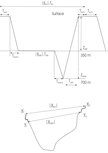
The motion of the profiler is simulated through an off-line algorithm obtained modifying the original code ARIANE (http://www.ifremer.fr/lpo/blanke/ARIANE/index.htmlBlanke and Raynaud, 1997). During a profiler cycle (see Fig. 1) the simulated profiler down-wells to a specified depth Z_drift where it freely drifts for a given time T_drift, then further

(7)

OSD

3, 1747–1790, 2006

Full Screen / Esc

downwells to a second specified depth Z_down to immediately upwell to the surface, where it stays for a given time T_surf. During the vertical displacements the floats are subjected to the horizontal movements induced by the vertical velocity shear. For the real profilers of the MedARGO program the “parking” depth Z_drift was chosen to be fixed at 350 m, that approximately corresponds to the “mean core depth” of the

Lev-5

antine Intermediate Water, while the deepest depth is fixed at 700 m (Poulain et al., 2005). Coherently, in each numerical experiment the same parking and the deepest depths were fixed while, during the vertical displacements, the “numerical profilers” move with the constant experimental-like downward and upward velocities w=−5 cm/s and w=10 cm/s, respectively.

10

In each cycle the profiler stays at surface for a time T_surf=T_surf1+T_surf2+T_surf3 where

T_surf1=T_surf2≈15 min represent, respectively, the time intervals between the last surface positioning and the sinking and between the resurfacing and the first satellite position-ing of the float and T_surf3≈6 h is the time spent at surface to transmit data.

The time interval T_tot between the last float positioning in the surface and the first

15

positioning after the re-surfacing is given (see Fig. 1) by:

T_tot = T_surf1+ T_down1+ T_drift+ T_down2+ T_upw+ T_surf2,

where T_down1=T_down2=350 m

5 cm/s≈2 h is the time necessary fort the first (from surface to

350 m) and the second (from 350 to 700 m) upwelling and T_upw= 700 m

10 cm/s≈2 h is the

time necessary for the upwelling of the profiler to the surface. During the horizontal

20

and vertical movements the profiler trajectory is sampled every 3 h and every 18 s., respectively. The code is flexible and the user can easily change the depth and time characteristics of the cycle that, together with the position of the initial conditions, are specified in a input ASCII file while two output files contain the floats trajectories and the vertical TS profiles.

25

We have performed 6 experiments making vary the time T_drift from 3 to 30 days. In each experiment 40 136 “numerical profilers” are uniformly released at surface (with an approximate density of 4 particles/100 km2) only where the bottom sea is deeper

(8)

OSD

3, 1747–1790, 2006

Full Screen / Esc

than 700 m except than in the North Aegean and Adriatic Sea and the Sicily Channel (see Fig. 2). After the release each numerical profiler sinks to the equilibrium depth of 350 m and starts its cycles. The integration is performed for 364 days using the 3 days mean eulerian hindcast velocity field of the year 2000 (52 weeks) of MFSPP obtained with the Med831 model (MOM 1/8◦×1/8◦×31, model details are described in Korres at

5

al., 2000 and Demirov et al., 2003).

When a real ARGO float crashes on the bottom it simply stays at the floor sea for the described time and then it resurfaces. In our simulations, if the numerical profiler reaches the bottom it immediately resurfaces to start a new cycle and, to avoid spurious results, we consider in our statistics only cycles in which the numerical floats do not

10

reach the bottom. Consequently we have a statistics based on a number of cycles

N_cycles6=N_tc=N_part·TINT

Ttot, where Npart is the number of profilers and TINT=364. For each

experiment N_cycles is always very large (see Table 1) and the ratio N_Ncycles

tc is about 0.66

for EXP1 and about 0.75 for the five experiments EXP2-EXP6.

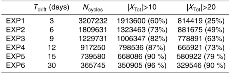
A proxy for the number of independent observations of vertical profiles of TS,

mea-15

sured during vertical movements, is given by the number of cycles characterized by having|X_Tot| >R₀, where R₀is the Rossby deformation radius that in the Mediterranean Sea is of the order of O(5–15) km. In the two last columns of Table 1, we show the number of cycles in which|X_Tot| is greater than 10 and 20 km. The percentage of “in-dependent” observations tends to saturate to 100% only for very big T_drift. For T_drift=6

20

(9)

OSD

3, 1747–1790, 2006

Full Screen / Esc

2.2 Sub-surface velocities

The estimate of the intermediate currents by means of ARGO floats is given by

U = X Tot T_tot = X 2− X1 T_tot , (1)

where X_i are the surface positions before and after the deep cycle of the float and T_tot is the time interval between these two subsequent, satellites located, surface points

5

(see Fig. 1).

The estimate of the intermediate velocity (Eq. 1) is inadequate when T_drift is greater or comparable to the intermediate velocity Lagrangian correlation time T_L since in this case, due to the presence of eddies and meanders, the length of the piece of trajectory D = RT_Tj+Tdrift

j d Y covered by the profiler in the time Tdrift is greater than

10 X_drift = Y₂−Y₁

, where Y_i represent coordinates of the first and last point of the trajectory at the parking depth Z_drift. A second source of inaccuracy is given by the fact that the definition (1) does not take into account the horizontal displacements occurring at the surface, first and before the satellite locations, and during the vertical motions of the profiler (X Tot 6= X drift

in the notation of Fig. 1).

15

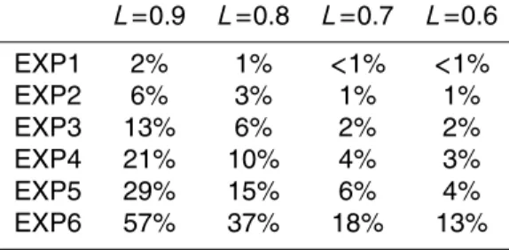
We have then computed for each cycle of each experimentX_drift

and the distance

D covered by the numerical profilers, approximated as a broken line of segments of

time length equal to the time interval of the Lagrangian integration (3 h). From Table 2, where we report for each experiment the percentage of cycles in which the ratio |Xdrift|

D

is smaller than a threshold value L, it is possible to see that a significant number of

20

cycle (>5%) have an important difference (L<0.8) for T_drift≥9 days, time scale that may be considered as a crude estimate of the order of magnitude of T_Lfrom the numerical Lagrangian velocity time series at 350 m.

The same experiments are used to assess the role of the vertical velocity shear and surface motions computing for each cycleX

Tot

,X

drift

and the error on the estimate

25

(10)

OSD

3, 1747–1790, 2006

Full Screen / Esc

of the intermediate velocity that is defined as: ∆(Tdrift)= X_Tot − X_drift X_drift . (2)

This huge statistics is then used to directly quantify the dependence of∆ on T_driftand to define possible criteria to decrease the error (2) or to identify geographical area where the vertical shear gives raise to smaller error∆.

5

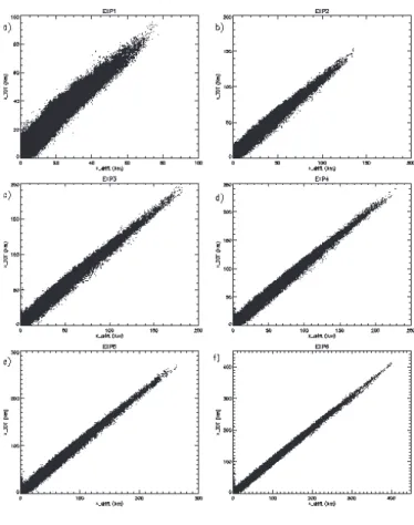
In Fig. 3 we show the scatter plot ofX_Tot vs.

X_drift

computed for each cycle of the six experiments EXP1-EXP6. As is expected, increasing T_drifthe plot is less “scat-tered” and the correlation betweenX

drift and X Tot

is more pronounced. However, due to the existence in each experiment of cycles with smallX

drift

and very big∆, the corresponding mean errors are very high (Table 3), the standard deviation of∆ largely

10

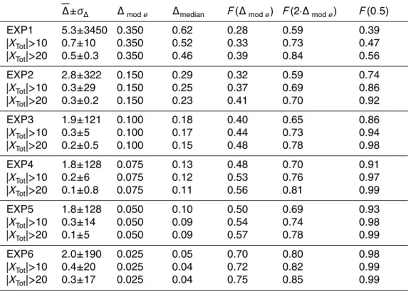
exceeds its mean value and the probability density function (pdf) P (∆) of ∆ (Fig. 4), even if characterized by well defined peak (“mode” value) for relatively low values of∆, have very long tails. In such situation it is interesting and useful to consider also sta-tistical indices from the cumulative F ( ˆ∆)= R∆₀ˆ P (∆)d∆, which represents the probability

to have a value∆< ˆ∆. Looking at these indices in Table 3 we can see that,

consid-15

ering all the cycles of the 6 experiments EXP1-EXP6 the mode varies from 0.350 to 0.025, the median (F (∆_median)=0.5) from 0.62 to 0.05 and the probability to have an error smaller than 50% (F (0.5)) from 39% to 98%. Moreover, considering only cycles in which the surface displacementX

Tot

is greater than 10 and 20 km the estimate on the intermediate velocity definitely improves. For instance if in EXP2 we consider only

20

cycles withX

Tot

>10 km (20 km) we have that 50% of cycles have an error less than

0.25 (0.23) and that the 37%, 69% and 86% (41%, 70% and 92%) of cycles give an estimate of the intermediate velocities with an error smaller than 0.15, 0.30 and 0.50 (F (∆_Mode), F (2·∆_Mode) and F (0.5)), respectively. Neglecting cycles with small X

Tot

(the only experimental observable variable) is only a first guess in order to attempt to

25

avoid floats with weak intermediate current. In a barotropic situation a smallX_Tot im-plies a smallX

drift

and considering only cycles with X

Tot

(11)

OSD

3, 1747–1790, 2006

Full Screen / Esc

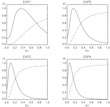
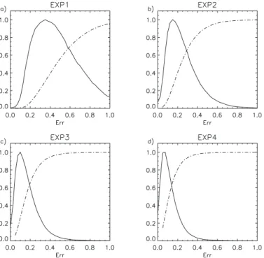
value may help to avoid pathological situation of floats moving very slowly; however, in presence of strong shear it is possible to have smallX

drift with large X Tot . In Fig. 5 we show the pdf of ∆ together with its cumulative computed considering only cycles withX_Tot

>20 km for the four experiments EXP1-EXP4.

Obviously the error decreases when the time T_drift increases but since the primary

5

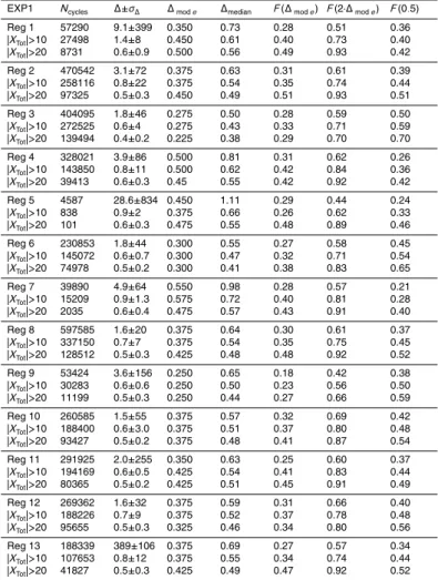
aim of the MedARGO experiment was the collection of the maximum number of inde-pendent TS vertical profiles, and since the assimilation procedure of positions in an OGGM requires that the parking time T_drift<T_L in the following we will analyze results only from EXP1 and EXP2. In particular, to identify a possible dependence of ∆ on the geographical position, we report in Tables 4 and 5 for EXP1 and EXP2, the

val-10

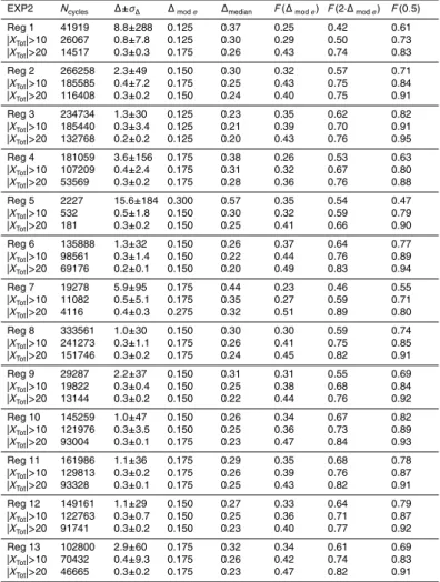
ues of ¯∆±σ_∆, ∆_Mode, ∆_MedianF (∆_Mode), F (2·∆_Mode) and F (0.5) computed considering cycles in the 13 regions indicated in Fig. 2. In all the regions, both for EXP1 and EXP2, the presence of cycles characterized by very small|X_drift| biases the statistics toward very high mean values of∆ and for EXP2 (Table 5) ∆_Median ranges from 0.23 to 0.57 (Regions 3 and 5) and the probability of having an estimate of the intermediate

veloc-15

ity with an error <0.5 (F(0.5)) varies from the 47% (Region 5) to the 82% (Regions 3 and 10). As expected, the situation improves considering cycles with|X_Tot| >10 km and |X_Tot| >20 km. In this latter case the standard deviation is smaller than the mean values almost everywhere and for EXP2∆_Median ranges from 0.20 (Regions 3 and 6) to 0.32 (Region 7) and we have that the probability of having an estimate of the intermediate

20

velocity with an error <0.5 (F(0.5)) varies from the 80% (Region 7) to the 95% (Re-gion 3). This re(Re-gional analysis shows that the estimate of the intermediate velocities is characterized by a smaller error in the North Western Mediterranean Sea (NWM) in the Northern Ionian (Regions 3 and 6) and in Western Levantine basin (Regions 10 and 11 while the Tyrrhenian and the Adriatic Seas and the Sicily Channel are expected to be

25

characterized by a larger error. In Fig. 6 we map for EXP2 the mean error∆ computed averaging, on a grid of 0.25◦×0.25◦, between all the error values of the cycles with X Tot >10 km and X Tot

>20 km falling in a given bin. From this figure we may also

see that all the area north to the African coast (influenced by the flow of the Modified 1756

(12)

OSD

3, 1747–1790, 2006

Full Screen / Esc

Atlantic Water which gives rise to a strong velocity shear) is characterized by a greater error on the estimate of the intermediate velocities.

Finally, in Fig. 7 we show the initial conditions of the numerical ARGO floats charac-terized by having∆<0.25, where now ∆ is the mean error computed on all the cycles of the entire 1 year long trajectory. Once again, this figure indicates that numerical

5

simulations suggest that the NWM, the Ionian Sea together with the Levantine basin are favorite sites for the deployment of ARGO profilers in order to have smaller error on the estimate of sub-surface velocities.

We conclude this section noting that the analysis of numerical profilers performed in WP4 of MFSTEP other than indicating areas where one can expect a smaller error on

10

the estimate of subsurface velocities were useful to define the parking time T_drift for the real profilers that was finally chosen to be equal to 5 days (Poulain et al., 2005), since this values is as a good compromise between the different and contrasting needs of having the larger number of independent observations, a small error on the estimate of the intermediate velocities and a time length of the profiler cycle smaller than the

15

intermediate velocities decorrelation time T_L.

3 Numerical surface particles: variability of the Lagrangian dispersion (WP8)

We present here some results related to the study of the interannual and seasonal vari-ability of the surface dispersion in the Mediterranean Sea obtained utilizing the MFS archive of Eulerian velocity field from 2000 to 2004. Lagrangian trajectories of

parti-20

cles were computed using the off-line ARIANE algorithm (Blanke and Raynaud, 1997, http://www.univ-brest.fr/lpo/ariane) in which, to mimic the behaviour of floating objects, the numerical particles are kept at the sea surface imposing null vertical velocity.

(13)

OSD

3, 1747–1790, 2006

Full Screen / Esc

3.1 Seasonal maps of surface dispersion

Seasonal variability of surface dispersion was investigated systematically integrating numerical particles using the daily averaged MFS hindcast Eulerian velocity fields over January 2000–December 2004 (MOM 1/8◦×1/8◦×31, Korres at al., 2000 and Demirov et al., 2003). Every week, about 400 000 particles (25 particles per model grid cell)

5

are uniformly released over the whole Mediterranean Sea surface, except within a 2-gridcell band adjacent to the coastline, and their trajectories are integrated for 28 days. The starting dates were lagged by a weekly interval over the first 10 weeks of each 13-week-long season to have each experiment embedded in the same season. Given the length of the time series (5 years), a total of 200 experiments (5 years × 4 seasons

10

× 10 experiments) were performed and this huge Lagrangian dataset was used to construct seasonal dispersion maps obtained by averaging the results over the five year considered (Pizzigalli et al., 20062). The statistics of dispersion properties over the entire surface of the Mediterranean Sea is calculated from the time evolution of “clusters” of numerical particles released and the results are available in a user friendly

15

web site (http://clima.casaccia.enea.it/riskmap) in terms of both global and local maps showing, respectively, the seasonal variability of the dispersion properties in a synoptic view (“basin-scale maps”) and as a function of the initial conditions.

This seasonal statistics was obtained by considering “ideal particles” that are con-strained to drift at the sea surface without being influenced by any of the physical

20

constraints (as drag or buoyancy changes) that affect most of the real Lagrangian ob-jects or tracers. Despite these strong restrictions, the obtained results may still be useful for practical situations since they provide the user with an immediate estimate of the variability of dispersion properties for “ideal particles” released at a given location before running (or in lack of) model simulations taking into account specific

character-25

istics of the searched object (e.g. Hackett et al. (2004) in the search and rescue activity or Zodiatis et al. (2006), for oil spills). In the same work numerical Lagrangian sur-face dispersion was checked against real data from the Mediterranean Sursur-face Drifter

(14)

OSD

3, 1747–1790, 2006

Full Screen / Esc

Database (1986–1999) (Poulain et al., 2001) by computing, for each season, the posi-tion error between the centres of mass of numerical particles and real drifters released with equivalent initial conditions.

We present here a further check against reality provided by a recent war event. In fact, during the last conflict in the Middle East (July–August 2006), the oil-fuelled

5

power plant of Jiyyeh, located directly on the coastline approximately 30 km south of Beirut, was hit by bombs on 15 July 2006. As a result, large part of the fuel was spilled into the Mediterranean Sea; the Lebanese ministry of environment estimated that approximately 10 000 tons of fuel oil were emitted into the sea in the fist hours and about 25 000 tons in the following 3 weeks (http://ec.europa.eu/environment/civil/

10

marin/mp01 en introduction.htm). The evolution of the oil spill has been monitored by remote sensing images and here we compare real oil dispersion with numerical es-timates in spite of the coastal origin of the oil. In fact, in the above mentioned work (Pizzigalli et al., 20062) and in the web site we do not compute statistics for particles released in the vicinity of coasts, since, due to the relatively low resolution, the OGCM

15

can not well represents coastal dynamics. In Fig. 8 we show (red lines) the centres of mass of each summer Lagrangian integration in which 225 particles are released in the grid point nearest to the power plant of Jiyyeh. The dark line represents the average on all the summer centres of mass and the integration is performed for 17 days since we dispose of a map on the first August 2006 of the oil location retrieved from a

satel-20

lite image acquired by the MODIS (MODerate resolution Imaging Spectroradiometer) sensor on board Terra satellite (courtesy of R. Sciarra, CNR-ISAC Rome). Numerical trajectories are superimposed on such map where green patches indicate the oil spill (see caption of Fig. 8 for details). Due to the coarse horizontal resolution (1/8◦×1/8◦) of the OGCM, the model coastlines do not coincide with the real ones (trajectories

25

may result to stay at land) and the point where numerical particles are released (black point in Fig. 8) is rather far from the real source of the spill. In spite of all these strong limitations from Fig. 8 we may observe that, even if the total centre of mass is slower, the numerical dispersion occurs in the same direction of the real oil spill and that the

(15)

OSD

3, 1747–1790, 2006

Full Screen / Esc

fastest centres of mass of a single Lagrangian integration of 225 particles (red lines) arrive near the coasts of Trabicus (about 100 km from the power plant) in 17 days, as in the case of the real oil spill. Obviously, better forecasting of dispersion may be obtained using coastal models forced with the winds of the considered days; however the inter-est of the proposed statistics of dispersion relies in the fact that it provides immediate

5

information in the entire basin.

3.2 Interannual variability of the Lagrangian transport in the Corsica and Sardinia Channels

We focus here our attention on the study of the interannual variability of the Lagrangian transport in two key areas of the surface circulation in the Western Mediterranean Sea:

10

the Sardinia and Corsica Channels. In the Sardinia Channel the near surface Modi-fied Atlantic Water (MAW) flows eastward and in proximity of Sicily bifurcates in two branches, one entering the Tyrrhenian Sea, the other flowing in the Eastern Mediter-ranean (EM) through the Sicily Channel (e.g., Astraldi et al., 1999). The MAW entering the Tyrrhenian Sea participates to its cyclonic surface circulation and it is subject to a

15

further bifurcation (Artale et al., 2006) in two branches, one recirculating in the Sardinia Channel, the other entering the Ligurian Sea through the Corsica Channel (approxi-mately 400 m deep) that is characterized by an highly variable, barotropic, northward flow of both surface water of Atlantic origin and intermediate water of eastern origin (Astraldi and Gasparini, 1992).

20

The study of the interannual variability of the path of the relatively fresher MAW in these two key areas is an important issue since both in the North Western Mediter-ranean (NWM) and in the EM occur deep water formation processes (among others MEDOC, 1970; Robinson and Golnaraghi, 1994; Mertens and Schott, 1998; Malanotte-Rizzoli et al., 1999), that are highly influenced by the surface water salinity.

25

Here we use the one day averaged MFS Eulerian velocity fields from 2000 to 2004 and we perform two experiments (CORS and SARD) in which, respectively, starting from January 2000 we release every week 12 354 and 11 980 particles in the two

(16)

OSD

3, 1747–1790, 2006

Full Screen / Esc

grid thick sections covering the Corsica and Sardinia Channels (see Fig. 9). Such particles are then integrated for 28 days for a total of 258 Lagrangian realizations. In experiment CORS particles are stopped if they recirculate in CORS or if they reach the section LIG while in experiment SARD they are stopped when arriving at the sections TYR and SIC or if they recirculate in SARD. We then construct a time series

repre-5

senting the variability of the surface section to section Lagrangian transport directly computing for each Lagrangian integration (realization) the number of particles that, after a given time, reach the ending sections. Some practical application may require the knowledge of the total integrated quantity of the tracer that reaches a given area in a given time. Consequently, in Fig. 10 we show as a function of time the percentage

10

of particles that reach the section LIG starting from section CORS after 28, 14 and 7 days (panels a, b and c). The thick black line represents the yearly averaged per-centage, while the thick red line is the percentage of realizations in which none of the particles reaches the ending section. The Lagrangian flow from the Corsica Channel toward the Western Ligurian Sea shows a well defined and realistic seasonality

(As-15

traldi and Gasparini, 1992) with maximum values in winter when from 2000 to 2003 for extended periods more than 80% of particles enter the Ligurian Sea in 28 days while few of them are able to arrive, during isolated events, in less than one week at the ending section LIG (Fig. 10c). From 2000 to 2004 the mean flow shows a decreasing trend and the yearly averaged percentage of particles reaching the LIG Section in 28

20

days (panel a) monotonically decreases from the 52% in 2000 to about 30% in 2004. This tendency is not evident for the faster isolated events while, for particles that arrive at the ending section in 14 days the percentage varies from about 20% for 2000 and 2001 to about 15% for 2004. It is interesting to observe that during these 5 years the number of realizations in which none of the particles released in the Corsica Channel

25

reaches the Ligurian Sea (red curves) in 14 and 28 days increases almost monoton-ically and that during the summers 2003 and 2004 for a time period of 4-5 months do not exist a surface flow connecting the Tyrrhenian and the Ligurian basin in less than 28 days. These results agree with experimental observations from surface drifters

(17)

OSD

3, 1747–1790, 2006

Full Screen / Esc

released in the Tyrrhenian Sea in the context of the Italian project “Ambiente Mediter-raneo” (http://clima.casaccia.enea.it/murst/index.html). In particular, during 2003 26 drifters were deployed in the central part of the basin and only 2 of them (released in the late autumn) were able to exit the Tyrrhenian, entering the Ligurian Sea (Rinaldi, 2006).

5

In Figs. 11 and 12 we show, respectively, the analogous plots for the surface flow connecting the Sardinia Channel to the Tyrrhenian Sea (Section TYR in Fig. 9) and the EM (Section SIC in Fig. 9). In both cases it cannot be observed a clear seasonality of the signal, even if the isolated events of fast particles reaching the EM in less than one week are mainly concentrated in the winter months (panel c of Fig. 12). In accord

10

to the CORS experiment, even the surface flow entering the Tyrrhenian Sea from the Sardinia Channel shows a general decreasing tendency from 2000 to 2004 and the percentage of particles that reach the TYR Section in 28 days varies from about 30% in 2000 to about 15% in 2004. The same behaviour it is not observed in the surface flow entering the EM (Fig. 12) that shows a maximum value during 2002 in which

15

more than 45% of particles reaches the ending section SIC. In this year the number of particles entering the EM in 28 days is almost five times the number of particles entering the Tyrrhenian Sea, as is possible to see in panel a of Fig. 13 where is plotted the ratio between the yearly averaged percentage of particles entering the Tyrrhenian and the EM. For slow particles (red and black lines in Fig. 13a) the mean value of this

20

ratio shows a rather high variability around its mean value (about 0.6–0.7) that is very similar to the estimate obtained both from experimental data and numerical simulation (e.g., Herbaut et al., 1996; Pierini et al., 2001). On the contrary, the number of fast particles is definitively larger for the flow connecting the Sardinia Channel to the EM (line blue in panel a of Fig. 13), since only in few (5) Lagrangian realizations particles

25

released in the Sardinia Channel are able to reach the TYR section in less than one week (panel c of Fig. 11). Finally, it is interesting to note that even if the ratio between the yearly averaged percentage of particles arriving at TYR and SIC in less than 28 and 14 days is almost always smaller than one (except than in 2000), we may observe the

(18)

OSD

3, 1747–1790, 2006

Full Screen / Esc

presence of a non negligible number of Lagrangian realizations in which most of the particles enter the Tyrrhenian Sea as is evident from panels b and c of Fig. 13 where for each realization is plotted the ratio between the particles reaching the TYR and the SIC section.

Other interesting information may be obtained from the arrival times in the ending

5

sections. Considering all the Lagrangian integrations, we may construct a five years long time series representative of the time behavior of the parameter in which we are interested. In fact, depending upon the practical application, one may be interested in different parameters of the probability density function (pdf) P (t) of the arrival times in the ending section. For instance, if we are interested in the dispersion of a dangerous

10

pollutant we could be interested to know when it reaches for the first time a given location. Contrastingly, if we are interested to know for how much time a source of pollution contaminates a given location, we are interested in studying the extreme tail of the arrival times pdf, or, for the practical cases in which the concentration of the tracer is an important factor, the relevant parameter to be considered is the mode value of the

15

pdf.

As an example of a possible application, we plot in Fig. 14 the yearly averaged minimum times (time in which the first particle reaches the ending section, panel a), the mean and the median values of the arrival times to the ending section (panel c and d). It has to be stressed that, since these characteristic times are computed considering only

20

particles reaching the final sections, the interpretation of their time behavior has to be

weighted with the results shown in Figs. 10–12, where we explicitly plot the percentage

of realizations in which none of the particles reach the ending sections. From Fig. 14 it is possible to observe that the characteristics times of the transport to the SIC and LIG (red and blue lines) sections oscillates around their mean values (please note that

25

in the CORS experiment the number of particles that do not reach the ending section strongly increases in 2003 and 2004) while all the characteristics times of the surface Lagrangian transport from the Sardinia Channel to the Tyrrhenian Sea (black line) show a tendency to increase during these years of about a 30%.

(19)

OSD

3, 1747–1790, 2006

Full Screen / Esc

3.2.1 Exponentially decaying particles

The variability of trend in the characteristic times of the Lagrangian transport may have important consequences when considering tracers which concentration decays with time. Till now we have considered particles representative of an ideal passive tracer that freely follows the surface flow without any change in its physical properties.

Con-5

trastingly, a chemical tracer may be subjected to evaporation and also to changes in its buoyancy characteristics. For instance, oil evaporation rate is a rather complex function of time strongly depending from its quality and type. In another context, taking in to ac-count a “mortality” rate of particles is crucial in the assessment of the larval exchange among marine communities, an important scientific issue, also for the management

10

of the fishery stocks and marine reserves. In fact, most marine species have a larval stage and, in particular, planktotrophic larvae are subjected to a wide dispersal since they may drift in the photic zone for a time varying from ten days to two months (Siegel et al., 2003). During this period larvae are subjected to a rate of mortality, depending on variable resources and predation processes, that is usually represented by a

con-15

stant coefficient, ranging from O(1) to O(30 days) (Cowen et al., 2000), which leads to an exponentially decay of their concentration.

When dealing with practical applications, it is then essential to take into account the time dependency of the biological or chemical element we consider. As an example of further applications and without entering in the details of the different tracer’s

phe-20

nomenology, we consider here the simplest case in which the advected particles are subjected to a “mortality” represented by the exponential decay e−tτ _{with folding time}

τ. Assuming that the “mortality” affects particles homogeneously and independently of

their location we may directly compute for each Lagrangian integration the pdf ˆP_τ(t)of the arrival times of particles representative of a tracer with concentration decaying with

25

the e-fold time τ by: ˆ

P_τ(t)= P (t) · e−tτ , (3)

where P (t) is the single Lagrangian realization pdf of the arrival time for particles no 1764

(20)

OSD

3, 1747–1790, 2006

Full Screen / Esc

subjected to mortality. For each realization, the number of the particles reaching the ending section is given by:

ˆ N_τ(t)= t Z 0 ˆ P_τ(t0)d t0= t Z 0 P (t0) · e−t0τ _{d t}0_. ₍₄₎

In the limiting case of P (t0)→δ(t0), ˆN_τ(t) is equal to N(t)·e−t0τ _{, where N(t)}=

t

R

o

P (t0)d t0. As an example of application, we compute, for each Lagrangian realization of the

5

two previously described experiments, ˆN_τ(t) with τ equal to 7 and 14 days. In Fig. 15 we show the yearly averaged percentages of particles reaching the ending sections for τ=7, 14 days (black and red curves) and for the integration time t=7, 14 and 28 days (dashed, thin and thick curves). These plots, when considered in specific cases, may have an interest per se; here we restrict our analysis to some general comments

10

noting that the percentage of particles, characterized by a given mortality rate arriving to the ending section is linked to the characteristic times of the surface “section to section” transport shown in Fig. 14. For instance we may note that, contrastingly with the monotonically decreasing 28-days transport in section LIG shown in panel a of Fig. 10 (black curve), when we consider particles with decaying e-fold rate τ=7 days

15

we have, e.g., (Fig. 15a) that the transports in 2003 are greater than in 2002, since in this year (2002) the characteristics times of the transport are greater, as is possible to see from Fig. 14 (blue line). The same is true for the transport in TYR where the (non monotonic decrease) of transport (Fig. 11) is amplified (of about the 50% for, e.g. for τ=14 and t=14, Fig. 15b), when considering particles characterized by a given

20

mortality rate, due to the fact that the characteristic times of the transport from the SARD and TYR section monotonically increase from 2000 to 2004 (Fig. 14). These simple qualitative relations, obviously depending on the space and time scales, may have important and quantitative consequences in practical applications as, e.g., in the dynamics of the marine biota where often the migration and the survival of specific

(21)

OSD

3, 1747–1790, 2006

Full Screen / Esc

specie critically depend on the concentration of its larvae.

4 Summary and perspectives

In this work we have presented some results obtained during MFSTEP by means of numerical simulations of ARGO profilers (Sect. 2) and surface floating objects (Sect. 3). Simulations of ARGO floats were used to define the optimal time cycling

character-5

istics of the profilers to maximize independent observations of TS vertical profiles and to study the dependence of the error on the estimate of the intermediate velocity as a function of the parking time T_drift and of the geographical areas. The obtained results have suggested that the choice T_drift=5 days is as a good compromise between the dif-ferent and contrasting needs of having the larger number of independent observations,

10

a small error on the estimate of the intermediate velocities and a time length of the profiler cycle smaller than the intermediate velocities decorrelation time T_L. Moreover, numerical simulations suggest that in the NWM, in the Ionian Sea and in the Levantine basin one can expect a smaller error on the estimate of subsurface velocities.

The MFS archive of the hindcast Eulerian velocity field was used to construct a

sur-15

face Lagrangian archive systematically integrating numerical particles released and constrained to drift at surface. In Sect. 3 we presented some results, concerning the study of the variability of the surface dispersion that was obtained from this huge La-grangian atlas. One of the main assumption of this approach is that the hindcast nu-merical velocity fields from MFS forecasting model, which assimilate in-situ real data

20

and are forced by high-resolution reanalyzed wind fields, represent the best basin-scale description available for eddy variability and quasi-steady circulation patterns. This tra-jectories data set was already used to build, following a statistical approach, seasonal maps of the surface dispersion (Pizzigalli et al., 20062). In this work, to test the skill of prediction of such, immediately available, seasonal dispersion maps we have shown a

25

further check against reality. Moreover we have provided a further example of exploita-tion of this Lagrangian data set investigating the interannual variability of the surface

(22)

OSD

3, 1747–1790, 2006

Full Screen / Esc

Lagrangian transport in two key areas of the Western Mediterranean, the Sardinia and the Corsica Channels. The “section-to section” Lagrangian transport was computed in a relatively short range of time (28 days) since this is the time scale of interest of most of possible practical applications. Lagrangian numerical simulations suggest a mono-tonic decreasing trend from 2000 to 2004 of the surface flow connecting the Tyrrhenian

5

Sea to the NWM. Moreover they show that during the summers 2003 and 2004, for an extended periods of 4–5 months, no particles are able to enter the Ligurian Sea in less than 28 days. These results suggest that the variability of the surface MAW flow from the Tyrrhenian has to be considered as a one of the possible cause of the variability of the hydrological properties observed in the NWM (Herbaut et al., 1997).

10

On the other hand, the surface flow from the Sardinia Channel shows a rather high variability of the ratio between the yearly averaged percentage of particles that reach the Tyrrhenian Sea and the EM around its mean value that, for relatively slow particles results to be about 0.6–0.7. However, the Lagrangian analysis shows the presence of a non negligible number of Lagrangian realizations in which most of the particles enter

15

the Tyrrhenian Sea, probably due to the wind forcing. An interesting development of the analysis presented here that definitively could improve the knowledge of the phe-nomenology of the surface dispersion relies in a systematic analysis of the correlation between wind regimes and path of advected numerical particles.

Finally we have computed the Lagrangian surface transport between the same

sec-20

tions considering particles characterized by an inner rate of mortality. The results shown have to be considered solely as an example of a little step toward more specific applications regarding chemical tracers or biological material dispersal. Further steps toward more realistic applications could be obtained refining this approach consider-ing, e.g., the dispersal of classes of planktotrophic larvae of specific interest for the

25

Mediterranean Sea with a rate mortality depending on the particle paths and on the hydrological properties, or inserting a prescribed downward vertical velocity represen-tative of the change of the buoyancy of the tracer.

(23)

OSD

3, 1747–1790, 2006

Full Screen / Esc

methodology useful to attain a better knowledge of the surface dispersion properties in the Mediterranean Sea through a simple integration of the MFS Eulerian velocity fields. In particular it could be of possible interest to insert, after having selected some key areas of the Mediterranean where compute the Lagrangian transport on such time scale (O(month)), such kind of analysis in the Mediterranean monthly bulletin

5

http://www.bo.ingv.it/mfs/monthly.htmprovided by now by the Italian Group of Opera-tional Oceanography (GNOO,http://www.bo.ingv.it/gnoo/) .

Acknowledgements. This work been carried in the framework of the projects MFSTEP, funded

by European Commission V Framework Program Energy, Environment and Sustainable De-velopment, and ADRICOSM, funded by Italian Ministry for the Environment and Territory. We

10

thank A. Anav for useful discussion about life and dead of larvae, R. Sciarra for the helpful support about the satellite image and E. Lombardi and A. Iaccarino for their invaluable support in the management of million of particles.

References

Artale, V., Calmanti, S., Pisacane G., and Rupolo, V.: The Atlantic and Mediterranean Sea as

15

connected systems, in: Mediterranean Climate Variability, edited by: Lionello, P., Malanotte-Rizzoli, P., and Boscolo, R., Amsterdam, Elsevier, 283–323, 2006.

Astraldi, M. and Gasparini, G. P.: The seasonal characteristics of the circulation in the North Mediterranean Basin and their relationship with the atmospheric-climatic conditions, J. Geo-phys. Res., 97, 9531–9540, 1992.

20

Astraldi, M., Baloupoulos, S., Candela, J., Font, J., Gacic, M., Gasparini, G. P., Manca, B., Theocharis, A., and Tintor `e, J.: The role of straits and channel in understanding the charac-teristics of Mediterranean circulation, Progress. Oceanogr., 44, 64–108, 1999.

Blanke, B. and Raynaud, S.: Kinematics of the Pacific equatorial undercurrent: a Eulerian and Lagrangian approach from GCM results, J. Phys. Oceanogr., 27, 1038–1053, 1997.

25

Cowen, R. K., Kamazima Lwiza, M. M., Sponaugle, S., Parisa C. B., and Olson, D. B.: Connec-tivity of Marine Populations: Open or Closed?, Science, 287, 857–859, 2000.

Demirov, E., Pinardi, N., Fratianni, C., Tonani, M., Giacomelli, L., and De mey, P.: Assimilation 1768

(24)

OSD

3, 1747–1790, 2006

Full Screen / Esc

scheme of Mediterranean Forecasting System: Operational implementation, Ann. Geophys., 21, 189–204, 2003.

Griffa, A., Molcard, A., Raicich, F., and Rupolo, V.: Assessment of the impact of TS assimilation from ARGO floats in The Mediterranean Sea, Ocean Sci. Discuss., 3 ,671–700, 2006. Guinehut, S., Larnicol, G., and Le Traon, P. Y.: Design of an array of profiling floats in the North

5

Atlantic from model simulations, J. Mar. Syst., 35, 1–9, 2002

Hackett, B., Breivik, Ø., and Wettre, C.: Forecasting the drift of things in the ocean, In Proceed-ings of the Second Symposium on the Global Ocean Data Assimilation Experiment, 1–3 November 2004, St. Petersburg, Florida, 2004.

Herbaut, C., Mortier, L., and Cr ´epon, M.: A sensitivity study of the general circulation of the

10

western Mediterranean Sea. Part I: The response to density forcing through the straits, J. Phys. Oceanogr., 26, 65–84, 1996.

Herbaut, C., Martel F. L., and Cr ´epon, M.: A sensitivity study of the general circulation of the western Mediterranean Sea. Part II: The response to atmospheric forcing, J. Phys. Oceanogr., 27, 2126–2145, 1997.

15

Korres, G., Pinardi, N., and Lascaratos, A.: The ocean response to low frequency interannual atmospheric variability in the Mediterranean Sea, J. Climate, 13, 705–731, 2000.

Malanotte-Rizzoli P., Manca, B. B., Ribera d’Alcal `a, M., Theocharis, A., Brenner, S., Budillon, G., and Ozsoy, E.,: The Eastern Mediterranean in the 80’s and in the 90’s: the big transition in the intermediate and deep circulations, Dyn. Atmos. Oceans, 29, 365–395, 1999.

20

Manzella, G. M. R., Scoccimarro, E., Pinardi, N., and Tonani, M.: Improved near-real time management procedures for the Mediterranean ocean Forecasting System? Volunteer Ob-serving Ships program, Ann. Geophys., 21, 49–62, 2003.

MEDOC group: Observation of Formation of Deep Water in the Mediterranean, Nature, 227, 1037–1040, 1970.

25

Mertens, C. and Schott, F.: Interannual variability of deep water formation in the Northwestern Mediterranean, J. Phys. Oceanogr., 28, 1410–1424, 1998.

Molcard, A., Griffa, A., and ¨Ozg¨okmen, T.,: Lagrangian data assimilation in multilayer primitive equation models, J. Atmos. Oceanic Technol., 22, 70–83, 2005.

Pierini, S. and Rubino, A.: Modeling the Oceanic Circulation in the Area of the Strait of Sicily:

30

The Remotely Forced Dynamics, J. Phys. Oceanogr., 31, 1397–1412, 2001.

Poulain, P. M., Mauri, E., Fayois, C., Ursella, L., and Zanasca P.,: Mediterranean surface drifter measurements from 1986 and 1999, CD-ROM, Naval Postgraduate school, Monterey-USA,

(25)

OSD

3, 1747–1790, 2006

Full Screen / Esc

2001.

Poulain, P. M.: A profiling float program in the Mediterranean Sea, Argonautics, 6, 2, 2005. Raicich, F.: The assessment of temperature and salinity sampling strategies in the

Mediter-ranean Sea: idealized and real cases, Ocean Sci., 2, 97–112, 2006.

Rinaldi, E.: Studio della circolazione superficiale del Mar Tirreno mediante dati satellitari e

5

Lagrangiani’ Tesi di Laurea,’ Universit `a La Parthenope, Napoli, 2006.

Robinson, A. R. and Golnaraghi, M.,: The physical and dynamical oceanography of the Mediter-ranean, in: Ocean Processes in Climate Dynamics: Global and Mediterranean Examples, edited by: Malanotte-Rizzoli, P. and Robinson, A. R., Kluwer Academic Publishers, The Netherlands, 255–306, 1994.

10

Siegel, D. A., Kinlan, B. P., Gaylord, B., Gaines, S. D.: Lagrangian descriptions of marine larval dispersion, Mar. Ecol. Progr. Ser., 260, 83–96, 2003.

Taillandier, V. and Griffa, A.: Implementation of position assimilation for ARGO floats in a re-alistic Mediterranean Sea OPA model and twin experiment testing, Ocean Sci. Discuss., 3, 255–289, 2006.

15

Zodiatis, G., Lardner, R., Hayes, D. R., Georgiou, G., Sofianos, S., Skliris, N., and Lascaratos, A.: Operational coastal ocean forecasting in the Eastern Mediterranean: implementation and evaluation, Ocean Sci. Discuss., 3, 397–434, 2006.

(26)

OSD

3, 1747–1790, 2006

Full Screen / Esc

Printer-friendly Version Interactive Discussion Table 1. T_drift, total number of cycles and number of cycles characterized by having |X_tot| greater

than 10 and 20 km for each experiment .In each experiment were integrated 40 136 numerical profilers uniformly released at surface.

T_drift(days) N_cycles |X_Tot|>10 |X_Tot|>20

EXP1 3 3207232 1913600 (60%) 814419 (25%) EXP2 6 1809631 1323463 (73%) 881675 (49%) EXP3 9 1229731 1006347 (82%) 778891 (63%) EXP4 12 917250 798536 (87%) 665921 (73%) EXP5 15 739580 668086 (90 %) 580922 (79 %) EXP6 30 365745 350905 (96 %) 329546 (90 %)

(27)

OSD

3, 1747–1790, 2006

Full Screen / Esc

Printer-friendly Version Interactive Discussion Table 2. Percentage of cycles characterized by a ratio |Xdrift|

D <L. L=0.9 L=0.8 L=0.7 L=0.6 EXP1 2% 1% <1% <1% EXP2 6% 3% 1% 1% EXP3 13% 6% 2% 2% EXP4 21% 10% 4% 3% EXP5 29% 15% 6% 4% EXP6 57% 37% 18% 13% 1772

(28)

OSD

3, 1747–1790, 2006

Full Screen / Esc

Table 3. Different statistical indices from the error (∆) pdf from the six experiments.

∆±σ_∆ ∆mod e ∆median F (∆mod e) F (2·∆mod e) F (0.5)

EXP1 |X_Tot|>10 |X_Tot|>20 5.3±3450 0.7±10 0.5±0.3 0.350 0.350 0.350 0.62 0.52 0.46 0.28 0.33 0.39 0.59 0.73 0.84 0.39 0.47 0.56 EXP2 |X_Tot|>10 |X_Tot|>20 2.8±322 0.3±29 0.3±0.2 0.150 0.150 0.150 0.29 0.25 0.23 0.32 0.37 0.41 0.59 0.69 0.70 0.74 0.86 0.92 EXP3 |X_Tot|>10 |X_Tot|>20 1.9±121 0.3±5 0.2±0.5 0.100 0.100 0.100 0.18 0.17 0.15 0.40 0.44 0.48 0.65 0.73 0.78 0.86 0.94 0.98 EXP4 |X_Tot|>10 |X_Tot|>20 1.8±128 0.2±6 0.1±0.8 0.075 0.075 0.075 0.13 0.12 0.11 0.48 0.53 0.56 0.70 0.76 0.81 0.91 0.97 0.99 EXP5 |X_Tot|>10 |X_Tot|>20 1.8±128 0.3±14 0.1±5 0.050 0.050 0.050 0.10 0.09 0.09 0.50 0.54 0.57 0.69 0.74 0.78 0.93 0.98 0.99 EXP6 |X_Tot|>10 |X_Tot|>20 2.0±190 0.4±20 0.3±17 0.025 0.025 0.025 0.05 0.04 0.04 0.70 0.72 0.75 0.80 0.82 0.85 0.98 0.99 0.99

(29)

OSD

3, 1747–1790, 2006

Full Screen / Esc

Table 4. EXP1: N_cycles, and statistical indices from the pdf of∆, in the different regions defined

in Fig. 2.

EXP1 Ncycles ∆±σ∆ ∆mod e ∆median F (∆mod e) F (2·∆mod e) F (0.5)

Reg 1 |XTot|>10 |XTot|>20 57290 27498 8731 9.1±399 1.4±8 0.6±0.9 0.350 0.450 0.500 0.73 0.61 0.56 0.28 0.40 0.49 0.51 0.73 0.93 0.36 0.40 0.42 Reg 2 |XTot|>10 |XTot|>20 470542 258116 97325 3.1±72 0.8±22 0.5±0.3 0.375 0.375 0.450 0.63 0.54 0.49 0.31 0.35 0.51 0.61 0.74 0.93 0.39 0.44 0.51 Reg 3 |XTot|>10 |XTot|>20 404095 272525 139494 1.8±46 0.6±4 0.4±0.2 0.275 0.275 0.225 0.50 0.43 0.38 0.28 0.33 0.29 0.59 0.71 0.70 0.50 0.59 0.70 Reg 4 |XTot|>10 |XTot|>20 328021 143850 39413 3.9±86 0.8±11 0.6±0.3 0.500 0.500 0.45 0.81 0.62 0.55 0.31 0.42 0.42 0.62 0.84 0.92 0.26 0.36 0.42 Reg 5 |XTot|>10 |XTot|>20 4587 838 101 28.6±834 0.9±2 0.6±0.3 0.450 0.375 0.475 1.11 0.66 0.55 0.29 0.26 0.48 0.44 0.62 0.89 0.24 0.33 0.46 Reg 6 |XTot|>10 |XTot|>20 230853 145072 74978 1.8±44 0.6±0.7 0.5±0.2 0.300 0.300 0.300 0.55 0.47 0.41 0.27 0.32 0.38 0.58 0.71 0.83 0.45 0.54 0.65 Reg 7 |XTot|>10 |XTot|>20 39890 15209 2035 4.9±64 0.9±1.3 0.6±0.4 0.550 0.575 0.475 0.98 0.72 0.57 0.28 0.40 0.43 0.57 0.81 0.91 0.21 0.28 0.40 Reg 8 |XTot|>10 |XTot|>20 597585 337150 128512 1.6±20 0.7±7 0.5±0.3 0.375 0.375 0.425 0.64 0.54 0.48 0.30 0.35 0.48 0.61 0.75 0.92 0.37 0.45 0.52 Reg 9 |XTot|>10 |XTot|>20 53424 30283 11199 3.6±156 0.6±0.6 0.5±0.3 0.250 0.250 0.250 0.65 0.50 0.44 0.18 0.23 0.27 0.42 0.56 0.66 0.38 0.50 0.59 Reg 10 |XTot|>10 |XTot|>20 260585 188400 93427 1.5±55 0.6±3.0 0.5±0.2 0.375 0.375 0.375 0.57 0.51 0.48 0.32 0.37 0.41 0.69 0.80 0.87 0.42 0.48 0.54 Reg 11 |XTot|>10 |XTot|>20 291925 194169 80365 2.0±255 0.6±0.5 0.5±0.2 0.350 0.425 0.425 0.63 0.54 0.51 0.25 0.41 0.45 0.60 0.83 0.91 0.37 0.44 0.49 Reg 12 |XTot|>10 |XTot|>20 269362 188226 95655 1.6±32 0.7±9 0.5±0.3 0.375 0.375 0.325 0.59 0.52 0.46 0.31 0.37 0.34 0.66 0.78 0.80 0.40 0.48 0.56 Reg 13 |XTot|>10 |XTot|>20 188339 107653 41827 389±106 0.8±12 0.5±0.3 0.375 0.375 0.425 0.69 0.55 0.49 0.27 0.34 0.47 0.57 0.74 0.92 0.34 0.44 0.52 1774

(30)

OSD

3, 1747–1790, 2006

Full Screen / Esc

Printer-friendly Version Interactive Discussion Table 5. EXP2: N_cycles, and different statistical indices from the pdf of ∆, in the different regions

defined in Fig. 2.

EXP2 Ncycles ∆±σ∆ ∆mod e ∆median F (∆mod e) F (2·∆mod e) F (0.5)

Reg 1 |XTot|>10 |XTot|>20 41919 26067 14517 8.8±288 0.8±7.8 0.3±0.3 0.125 0.125 0.175 0.37 0.30 0.26 0.25 0.29 0.43 0.42 0.50 0.74 0.61 0.73 0.83 Reg 2 |XTot|>10 |XTot|>20 266258 185585 116408 2.3±49 0.4±7.2 0.3±0.2 0.150 0.175 0.150 0.30 0.25 0.24 0.32 0.43 0.40 0.57 0.75 0.75 0.71 0.84 0.91 Reg 3 |XTot|>10 |XTot|>20 234734 185440 132768 1.3±30 0.3±3.4 0.2±0.2 0.125 0.125 0.125 0.23 0.21 0.20 0.35 0.39 0.43 0.62 0.70 0.76 0.82 0.91 0.95 Reg 4 |XTot|>10 |XTot|>20 181059 107209 53569 3.6±156 0.4±2.4 0.3±0.2 0.175 0.175 0.175 0.38 0.31 0.28 0.26 0.32 0.36 0.53 0.67 0.76 0.63 0.80 0.88 Reg 5 |XTot|>10 |XTot|>20 2227 532 181 15.6±184 0.5±1.8 0.3±0.2 0.300 0.150 0.150 0.57 0.30 0.25 0.35 0.32 0.41 0.54 0.59 0.66 0.47 0.79 0.90 Reg 6 |XTot|>10 |XTot|>20 135888 98561 69176 1.3±32 0.3±1.4 0.2±0.1 0.150 0.150 0.150 0.26 0.22 0.20 0.37 0.44 0.49 0.64 0.76 0.83 0.77 0.89 0.94 Reg 7 |XTot|>10 |XTot|>20 19278 11082 4116 5.9±95 0.5±5.1 0.4±0.3 0.175 0.175 0.275 0.44 0.35 0.32 0.23 0.27 0.51 0.46 0.59 0.89 0.55 0.71 0.80 Reg 8 |XTot|>10 |XTot|>20 333561 241273 151746 1.0±30 0.3±1.1 0.3±0.2 0.150 0.175 0.175 0.30 0.26 0.24 0.30 0.41 0.45 0.59 0.75 0.82 0.74 0.85 0.91 Reg 9 |XTot|>10 |XTot|>20 29287 19822 13144 2.2±37 0.3±0.4 0.3±0.2 0.150 0.150 0.150 0.31 0.25 0.22 0.31 0.38 0.44 0.55 0.68 0.76 0.69 0.84 0.92 Reg 10 |XTot|>10 |XTot|>20 145259 121976 93004 1.0±47 0.3±3.5 0.3±0.1 0.150 0.150 0.175 0.26 0.25 0.23 0.34 0.36 0.47 0.67 0.73 0.84 0.82 0.89 0.93 Reg 11 |XTot|>10 |XTot|>20 161986 129813 93328 1.1±36 0.3±0.2 0.3±0.1 0.175 0.175 0.175 0.29 0.26 0.25 0.35 0.39 0.43 0.68 0.76 0.82 0.78 0.87 0.91 Reg 12 |XTot|>10 |XTot|>20 149161 122763 91741 1.1±29 0.3±0.7 0.3±0.2 0.150 0.150 0.150 0.27 0.25 0.23 0.33 0.36 0.40 0.64 0.71 0.77 0.79 0.87 0.92 Reg 13 |XTot|>10 |XTot|>20 102800 70432 46665 2.9±60 0.4±9.3 0.3±0.2 0.175 0.175 0.175 0.32 0.26 0.23 0.34 0.42 0.47 0.61 0.74 0.82 0.69 0.83 0.91

(31)