HAL Id: hal-03060439
https://hal.archives-ouvertes.fr/hal-03060439
Submitted on 15 Jan 2021
HAL is a multi-disciplinary open access
archive for the deposit and dissemination of
sci-entific research documents, whether they are
pub-lished or not. The documents may come from
teaching and research institutions in France or
abroad, or from public or private research centers.
L’archive ouverte pluridisciplinaire HAL, est
destinée au dépôt et à la diffusion de documents
scientifiques de niveau recherche, publiés ou non,
émanant des établissements d’enseignement et de
recherche français ou étrangers, des laboratoires
publics ou privés.
landslide inventories: the weak influence of slope and
strong influence of total storm rainfall
Odin Marc, André Stumpf, Jean-Philippe Malet, Marielle Gosset, Taro
Uchida, Shou-Hao Chiang
To cite this version:
Odin Marc, André Stumpf, Jean-Philippe Malet, Marielle Gosset, Taro Uchida, et al.. Initial insights
from a global database of rainfall-induced landslide inventories: the weak influence of slope and strong
influence of total storm rainfall. Earth Surface Dynamics, European Geosciences Union, 2018, 6 (4),
pp.903-922. �10.5194/esurf-6-903-2018�. �hal-03060439�
https://doi.org/10.5194/esurf-6-903-2018 © Author(s) 2018. This work is distributed under the Creative Commons Attribution 4.0 License.
Initial insights from a global database of rainfall-induced
landslide inventories: the weak influence of slope and
strong influence of total storm rainfall
Odin Marc1, André Stumpf1, Jean-Philippe Malet1, Marielle Gosset2, Taro Uchida3, and Shou-Hao Chiang4
1École et Observatoire des Sciences de la Terre, Institut de Physique du Globe de Strasbourg, Centre National
de la Recherche Scientifique UMR 7516, University of Strasbourg, 67084 Strasbourg CEDEX, France
2Géoscience Environnement Toulouse, Toulouse, France
3National Institute for Land and Infrastructure Management, Research Center for Disaster
Risk Management, Tsukuba, Japan
4Center for Space and Remote Sensing Research, National Central University, Taoyuan City 32001, Taiwan
Correspondence:Odin Marc (odin.marc@unistra.fr)
Received: 5 March 2018 – Discussion started: 27 March 2018
Revised: 6 July 2018 – Accepted: 17 September 2018 – Published: 10 October 2018
Abstract. Rainfall-induced landslides are a common and significant source of damages and fatalities
world-wide. Still, we have little understanding of the quantity and properties of landsliding that can be expected for a given storm and a given landscape, mostly because we have few inventories of rainfall-induced landslides caused by single storms. Here we present six new comprehensive landslide event inventories coincident with well iden-tified rainfall events. Combining these datasets, with two previously published datasets, we study their statistical properties and their relations to topographic slope distribution and storm properties. Landslide metrics (such as total landsliding, peak landslide density, or landslide distribution area) vary across 2 to 3 orders of magnitude but strongly correlate with the storm total rainfall, varying over almost 2 orders of magnitude for these events. Ap-plying a normalization on the landslide run-out distances increases these correlations and also reveals a positive influence of total rainfall on the proportion of large landslides. The nonlinear scaling of landslide density with to-tal rainfall should be further constrained with additional cases and incorporation of landscape properties such as regolith depth, typical strength or permeability estimates. We also observe that rainfall-induced landslides do not occur preferentially on the steepest slopes of the landscape, contrary to observations from earthquake-induced landslides. This may be due to the preferential failures of larger drainage area patches with intermediate slopes or due to the lower pore-water pressure accumulation in fast-draining steep slopes. The database could be used for further comparison with spatially resolved rainfall estimates and with empirical or mechanistic landslide event modeling.
1 Introduction
Landslides associated with heavy rainfall cause significant economic losses and may injure several thousand people a year worldwide (Petley, 2012). In addition, the frequency of landsliding increases with the frequency of extreme rainfall events (Kirschbaum et al., 2012), which is expected to be enhanced by global climate change (Gariano and Guzzetti,
2016). Landslides are also recognized as a major geomorphic agent contributing to erosion and sediment yield in moun-tainous terrain (Hovius et al., 1997; Blodgett and Isacks, 2007). Yet, constraining quantitative relationships between landslides and rainfall metrics remains difficult.
There is limited theoretical understanding of how rain-fall, through water infiltration in the ground, can increase pore-water pressures and trigger failures (Van Asch et al.,
1999; Iverson, 2000). Therefore, a variety of mechanistic models have been developed, usually by coupling a shallow hydrological model to a slope failure criterium (e.g., Mont-gomery and Dietrich, 1994; Baum et al., 2010; Arnone et al., 2011; Lehmann and Or, 2012; von Ruette et al., 2013). How-ever, such deterministic approaches require not only appro-priate physical laws but also an accurate and fine-scale quan-tification of several input parameters such as topography, cohesion, permeability, and rainfall pattern (Uchida et al., 2011). In most places, such a level of detailed information is currently unavailable, rendering deterministic approaches hardly applicable.
Data-driven studies have mostly focused on using precise information on individual landslide location and timing to decipher thresholds, typically based on preceding rainfall intensity and duration, at which a landslide would initiate (Caine, 1980; Guzzetti et al., 2008, and references therein). Although useful for hazard and early-warning purposes (e.g., Keefer et al., 1987), these approaches do not address the quantity and properties of landslides that can be triggered by a rainfall event. In order to understand the importance of rainfall on erosion rates or to anticipate landslide hazard as-sociated with emerging cyclones and heavy rainstorms, it is highly desirable to quantitatively relate the properties of a landslide event L (total area, volume, size distribution) to the combination of site susceptibility, s, and rainfall forcing, f , properties, or equivalently to develop scaling relations of the form of
L = g(s(slope, soil thickness, strength, permeability, . . .), f(total rainfall, intensity, antecedent rainfall, . . .)). (1) Note that variables in such an equation may be a statistical description at the catchment or landscape scale (being a sim-ple mean or other moments of the distribution), and thus may not describe the fine-scale variability required by tic models. Although being simplified versions of mechanis-tic models, such scaling laws can be useful to describe aver-age properties of the phenomena, i.e., a population of land-slides associated with a constrained trigger. The advantage of statistical or semi-deterministic approaches is that they are able to accurately predict global properties, while circum-venting the difficulties of predicting specific local properties of individual landslides. Indeed, such scaling laws would al-low prediction in data-scarce regions and possibly at var-ious scales (hillslope scale, catchment scale, region scale, etc). This approach has driven important progress for both the understanding and hazard management of earthquake-induced landslides, thanks to the introduction of purely em-pirical, physically inspired, or mixed functional relations in the form of Eq. (1) (e.g., Jibson et al., 2000; Meunier et al., 2007, 2013; Nowicki et al., 2014; Marc et al., 2016, 2017). This progress has been possible thanks to detailed investiga-tion of individual case studies with comprehensive landslide event inventories (e.g., Harp and Jibson, 1996; Liao and Lee,
2000; Yagi et al., 2009) and through their combined analy-sis as aggregated databases (Marc et al., 2016, 2017; Tanya et al., 2017). By comprehensive event-inventories we mean that all landslides larger than a given size were mapped, and that the spatial extent of the imagery allowed us to observe the landslide density fading away in all direction, tracking the reduction of the forcing intensity of the triggering event, whether shaking or rainfall.
In contrast, few studies on rainfall-induced landslides are based on comprehensive event inventories. Some studies are based on individual landslide information. For example, Saito et al. (2014) studied 4744 landslides in Japan, that oc-curred between 2001 and 2011, to better understand which rainfall properties control landslide size. This dataset, ag-gregating a small subset of the landslides triggered by rain-fall events, misses the vast majority of landslides. For exam-ple, in Japan, Tropical Storm Talas alone caused a similar amount of landslides in a few days. It is, therefore, insuffi-cient for a more advanced statistical analysis. At the global scale, Kirschbaum et al. (2009) presented a catalog contain-ing information on 1130 landslide events worldwide, which occurred in 2003, 2007, and 2008. With this catalog, they underline the correlation between extreme rainfall and land-sliding (Kirschbaum et al., 2012). However, such catalogs, mainly based on reports from various kinds, are rarely ade-quate to constrain the quantity and properties of landslides triggered by a rainfall event. Thus, we consider that neither studies, based on a small sample of individual landslides or on a global-scale analysis, will be able to effectively con-strain Eq. (1), and that detailed storm-scale information is needed.
Few case studies rely on fragmentary event inventories (and are briefly reviewed in the next section) but they may contain too few landslides for statistical analyses or may be biased to specific locations (e.g., along roads or near settle-ments, within weak lithological units, or near rivers), thus complicating the deconvolution of forcing and site influ-ences. However, in theory, satellite imagery allows for com-prehensive mapping of landslides larger than the resolution limit, across all catchments affected by a large storm. In prac-tice, obtaining useful images strictly constraining the lands-liding caused by a single storm is not always possible, mainly because of cloud coverage, and detailed mapping across vast areas represents a significant work effort. As a result, land-slide inventories triggered by rainfall during a whole season or a few years are used for testing mechanistic models (e.g., Baum et al., 2010; Arnone et al., 2011).
The purpose for this work is to present a compilation of new and past comprehensive rainfall-induced landslide (RIL) inventories, each containing the landslide population associ-ated with an identified storm. They constitute the core of an expandable database, essential for further research. We first briefly review existing comprehensive and partially complete inventories associated with specific storms. Then we present six new inventories and analyze their statistical properties in
terms of size (total area, landslide density), geometry (length, width, and depth), and relation to topographic slopes. We fur-ther analyze and discuss these properties with respect to rain-fall observations in those cases and conclude on the various insights that can be derived from such an inventory compila-tion.
2 Data and methods
2.1 Review of pre-existing datasets
An in-depth literature review revealed that very few compre-hensive, digital, RIL inventories have been published, such as the Colorado 1999 and Micronesia 2002 events detailed below. If we look for partial inventories, in which landslides have been mapped comprehensively in limited zones affected by a storm, a few more datasets exist.
For example, Hurricane Mitch hit Central America at the end of 1998 and triggered thousands of landslides across several countries. The rainfall was record-breaking in many places, with rain gauges recording up to 900, 1100, and 1500 mm in Honduras, Guatemala, and Nicaragua (Bucknam et al., 2001; Cannon et al., 2001; Crone et al., 2001; Harp et al., 2002). In the following weeks, the USGS performed a number of aerial surveys, identified the most affected ar-eas in these three countries as well as in El Salvador (where the rainfall amount was less), and mapped a large number of the failures in selected zones. The resolution of their aerial photographs allowed them to distinguish failures down to a relatively small size (< 100 m2), but the mapping amalga-mated multiple failures into single polygons, and combined very long debris flow paths and/or channel deposits to the source areas. Because of these limitations, we did not inves-tigate this case in detail but note that these inventories may be corrected and used by later studies. Similarly in a number of studies, inventories of all the landslides caused by a given storm in a specific catchment or geographic zone can be found: in Liguria 2000 (Guzzetti et al., 2004), Umbria 2004 (Cardinali et al., 2006), Sicily 2009 (Ardizzone et al., 2012), Peru 2010 (Clark et al., 2016), Thailand 2011 (Ono et al., 2014), and Myanmar 2015 (Mondini, 2017), as well as in Taiwan for 10 typhoons between 2001 and 2009 (Chen et al., 2013). These inventories could not constrain the total land-slide response to a storm, but may allow to constrain relation-ships between landslide properties and local rainfall proper-ties, provided that enough landslides have been mapped for statistical analysis (e.g., > 50–100) and without any system-atic sampling bias. However, a detailed assessment of these dataset properties and of their relation to rainfall is outside the scope of this study although it would probably interest-ingly complement our work in the future.
In this study, we analyzed two datasets previously pub-lished by the USGS. First, afternoon rain on 28 July 1999 that triggered numerous landslides and debris flows in the Colorado Front Range (Godt and Coe, 2007). Based on aerial
photograph interpretation and field inspection, landslides were mapped as polygons containing source areas, debris flow travel, and deposition zones. Initiation points were as-sumed to be the highest point upslope of each mapped land-slide. In 57 out of 328 polygons, multiple initiation points (2 to > 15) were mapped for multi-headed polygons (Godt and Coe, 2007). These polygons are among the largest of the inventory and represent 61 % of the total landslide area. The surface of the source areas were often of similar width, suggesting equivalent contribution from each source to the transport and deposit areas, and rendering a manual splitting impractical. Thus, we instead conserve multi-headed poly-gons and we use the whole landslide area, Al, perimeter, Pl,
and number of source, Ns, for each multi-headed polygon
to derive an equivalent area and perimeter associated with each source: A∗l =Al/Ns and Ps=Pl/Ns. This first-order
approach underestimates the perimeter of each component by one width, the segment that would be added for each new subpolygon; however, this underestimation decreases with the length/width ratio of the polygons, and is already be-low 10 % for L/W > 4. In any case, this assumption does not affect the total area affected, but it changes the land-slide frequency-area and frequency-width distributions, and all terms derived from them.
The second dataset contains landslides caused by a sum-mer typhoon in July 2002, mapped exhaustively with aerial photos on the islands of Micronesia (Harp et al., 2004). We digitized the original maps based on strong contrast between red polygons and the rest of the maps. A few artifacts due to this image processing were removed and a few amalgams were split. Again, scarps and deposits are not differentiated.
2.2 New comprehensive inventories of rainfall-induced landslides
We present the mapping methodology and imagery (Table S1 in the Supplement) used to produce six additional invento-ries. Here we consider landslides as a rapid downslope trans-port of material, disturbing vegetation outside of the fluvial domain, which we define by visible water flow in the im-agery. We also consider individual landslides with a single source or scar areas to avoid amalgamation, and split poly-gons when necessary. Although the transition between hill-slopes and channel may be blurry and in part subjective, the width estimation (cf. Sect. 2.4) will mitigate variations in the transport length, as long as large alluviated or flooded ar-eas are not mapped as landslide deposits. Still the limit be-tween scar, transport, and deposit areas could rarely be de-tected with the available imagery, and all polygons consider the whole disturbed areas on the hillslopes. Subsets of the inventories in Taiwan 2009 and Brazil 2011 were produced with an automatic algorithm, and then edited and corrected manually, while all others were manually mapped.
In 2008 around the Brazilian town of Blumenau, several days of intense rainfall at the end of a very wet fall
trig-gered widespread landsliding and flooding, with some partial inventories published in the Brazilian literature (e.g., Poz-zobon, 2013; Camargo, 2015), which were not reported in the international literature. The detection and manual map-ping of landslides as georeferenced polygons was primarily done with a pair of Landsat 5 cloud-free images (1 Febru-ary 2009 and 2 March 2008). The coarse resolution (30 m) of the images allowed us to only locate vegetation distur-bances and accurate landslide delineation was only possible for the largest events. Therefore, we used extensive high-resolution imagery available in Google Earth (over > 90 % of the area of interest, AOI) acquired in May–June 2009 in most areas, and in 2010–2012 elsewhere, where scars were still visible. To avoid mapping post-event landslides, we only mapped the ones corresponding to vegetation radiometric in-dex (e.g., NDVI) reduction for the pair of Landsat 5 images, present even for subpixel landslides (e.g., 10 m×5 m). Thus, the landslide mapping could be confirmed for ∼ 90 % of the mapped polygons, and industrial digging or deforestation occurring on steep slopes could be avoided. This approach avoids amalgamating groups of neighboring landslides and allows for the mapping of very small landslides (∼ 1 pixel in Landsat 5 images). However, some detailed field mapping in the surrounding of Blumenau reports up to twice the number of landslides that we observed (Pozzobon, 2013), indicating that we still miss a substantial number of small events. Nev-ertheless, these landslides must be quite small (not visible in ∼1 m resolution imagery) and likely do not affect any of our statistics (area, volume, slope) apart from the total number of landslides.
The same approach was used to map the intense landslid-ing caused by a few days of intense rainfall between 10 and 12 January 2011 (Netto et al., 2013), in the mountains north-east of Rio de Janeiro. Near Teresópolis, first we used a pan-sharpened (10 m) EO-ALI and 30 m Landsat 7 images from February 2011 for co-registration and ortho-rectification.
>95 % of the slides were cross-checked in Google Earth based on images from the 20 and 24 January 2011 (Fig. 1); and where clouds or no images where available we mapped landslides directly from Google Earth (available over >90 % of the AOI), even if poor ortho-rectification may create geo-metric distortions. Closer to Nova Friburgo, we used a pair of very-high-resolution GeoEye-1 images (2/0.5 m resolu-tion in multispectral/panchromatic) from 26 May 2010 and 20 January 2011. On these images we applied the methods presented by Stumpf et al. (2014) to classify the whole im-age, detecting > 90 % of the landslides we could manually observe , but also including false positive. Thus, we man-ually screened the image to remove agricultural fields, inun-dated areas, channel deposits that were included, and split the amalgamated landslides frequently given the important clus-ters of landslides in many parts of the image. This correction seems sufficient given that the landslide size distribution for the three subparts of the inventory are consistent (Fig. S1 in the Supplement). Polygons from the automatic classification
display a slightly larger equivalent length/width ratio, maybe because some amalgamated polygons have been missed or simply because the classification allows for hollow polygons, biasing upward the length/width estimate based on a perime-ter/area ratio (cf. Sect. 2.4).
From 1 to 4 September 2011, Tropical Storm Talas poured heavy rainfall on the Kii Peninsula, in Japan, resulting in several thousands of landslides. For disaster emergency re-sponse, the National Institute for Land and Infrastructure Management of Japan (NILIM) mapped landslides across most of the affected areas based mainly on post-typhoon aerial photographs and occasionally on Google Earth im-agery (Uchida et al., 2012). Screening antecedent imim-agery (2010–2011) from Google Earth and Landsat 5, we identi-fied and removed a few hundred pre-Talas polygons, mostly within 5 km of 136.25◦E/34.29◦N and 135.9◦E/34.20◦. With Google Earth we could validate NILIM mapping over about 85 % of the AOI and we added almost 200 poly-gons in areas were aerial photographs were not taken and split many large or multi-headed polygons that were amal-gamated. Some polygons had distorted geometry or exagger-ated width, most likely due to poor ortho-rectification of the aerial imagery and/or time constraints for the mapping. We could not systematically check all polygons, but we checked and corrected all polygons larger than 30 000 m2(3 % of the catalog but representing 45 % of the total area). We consider that the remaining distortions for some of the smaller poly-gons have minor impacts on the statistics discussed in the next sections.
In Taiwan, we collected landslide datasets associated with the 2008 Kalmaegi (16–18 July) and 2009 Morakot (6– 10 August) typhoons, partially described by Chen et al. (2013). For 2008, we compared multispectral composite im-ages and NDVI changes between (30 m) Landsat 5 imim-ages taken on the 21 June, 7 July, and 23 July. The image from 7 July is covered by clouds and light fog in many parts but allows us to identify that most places affected by landslides in the last images were still vegetated at this time. Thus all new landslides are attributed to the rainfall from typhoon Kalmaegi. For 2009, landslides were mapped with pre- and post-event FORMOSAT-2 satellite images (2 m panchro-matic and 8 m multi-spectral; Chang et al., 2014). To cover most of the island, we mosaicked multiple mostly cloud-free pre-event (14 January, 8 May, 9 May, 10 May, 6 June 2009) and post-event (17 August, 19 August, 21 August, 28 Au-gust, 30 AuAu-gust, 6 September 2009) images. For a subsets of the inventory, especially to the east of the main divide, land-slides were significantly amalgamated and bundled with river channel alluviation. We thus manually split the polygons and removed the channel areas.
In a few areas with clouds (< 5 % of the AOI) in the post-event mosaic, we mapped with Landsat 5 images (from 24 June and 12 September 2009), even if the spatial resolu-tion limit may have censored the smallest landslides in these zones. Special attention was given to the separation of
in-Figure 1.Landslides inventory superimposed on digital surface model for the events in Japan 2011 (a), Colombia 2015 (b), Taiwan 2008 and 2009 (c), Brazil 2008 (d), Colorado 1999 (e), Micronesia 2002 (f) and Brazil 2011 (g). Landslides are in purple, rain gauges used in this study are in red dots (and red crosses for Taiwan 2009), and the yellow frames show the availability of high-resolution imagery (Google Earth) used to check or perform the mapping. In (c) the green dots are landslides from 2008, while purple dots are from 2009. In (g) purple, red, and green dots are landslides mapped from EO-ALI, Google Earth, and automatic classification of GeoEye images, respectively.
dividual landslides by systematically checking and splitting polygons above 0.1 km2(2 % of the catalog but representing 30 % and 60 % of the total area and volume, respectively). However, it is clear that a number of smaller landslides are missed or merged with large ones; and, therefore, although total landsliding and landslide locations on slopes may be well represented, the size distribution of this catalog must be biased to some extent.
Between 15 and 17 May 2015, heavy rainfall in the moun-tains above the village of Salgar, Colombia, triggered catas-trophic landslides and debris flow (> 80 deaths). Landslide mapping was carried out by comparing a (10 m) Sentinel-2 image from the 21 July 2016 and a pan-sharpened (15 m) Landsat 8 image from the 19 July and 26 December 2014.
These images were selected for their absence of clouds, good conditions of light, and similarity. High spatial resolution im-agery from Google Earth, dated from 31 May 2015, shows fresh scars consistent with our mapping over most of the area (Fig. 1), and we assumed that the remaining landslides (< 15 % of the inventory) were also triggered by the same rainfall event.
2.3 Rainfall data
Rainfall data quality and amount are very variable for the dif-ferent events, from none or one single gauge (for Microne-sia or Colombia) to a dense gauge network and potentially weather radar coverage in Japan, Taiwan, and Brazil.
There-fore, we selected a simple index that could be obtained for each case in order to discuss potential rainfall controls on the landslide properties. For each case we calculated an estimate of total rainfall, Rt, duration, D, and a peak rainfall
inten-sity over 3 h, I 3 (Table 1). Note that these variables do not represent an average value within the whole footprint of the storm, but rather a maximal forcing, usually colocated with the areas where landsliding was the most intense (Fig. 1) and derived mostly from one or a few rain gauges. Thus, these indexes may be taken as storm magnitude. A more detailed analysis of the spatiotemporal pattern of the rainfall and of its relations to the spatial pattern of landsliding is highly de-sirable, but challenging and is left for a future study.
The estimates from Taiwan and Japan are based on hourly gauge measurements from the Japan Meteorological Agency and Taiwan Institute for Flood and Typhoon research. In each case we took the three closest gauges within 5 to 15 km from the areas with the highest landslide densities (in 0.05 by 0.05◦window, Fig. S2) and computed their average prop-erties (Fig. 2). Minimum and maximum single gauge mea-surements give a coarse measure of the uncertainty. A sin-gle gauge is available in Micronesia, and we used the hourly rainfall from 1 to 3 July 2002 reported in Harp et al. (2004). For Colorado, we used the hourly rainfall from the rain gauge at Grizzly Peak, closest to the intense landsliding reported by Godt and Coe (2007). For this event, radar data indicate very localized, high-intensity precipitation located on the peaks where the debris flows occurred (Godt and Coe, 2007) and suggests that the single closest gauge is more representative than averaging with the other nearby ones. For the event in Brazil 2008 we considered the total daily rainfall from Luis Alves station (Fig. 1), where more than 130 mm day−1were accumulated on the 21, 22, and 23 November and 250 mm on the 25, and intensity going up to 50 mm h−1 (Camargo, 2015). These days were also preceded by an abnormally wet period, with November 2008 accumulating ∼ 1000 mm, 7 times the long-term average for this month. In 2011 in Brazil, hourly rain data at Sitio Sao Paulista report 200 mm in 8 h before gauge failure, while there, and at nearby sites, the cumulative rainfall was ∼ 280 mm from the 10 to the morn-ing of the 12 January (Netto et al., 2013). For these cases, rain gauges give a trustworthy estimate of the local rainfall, but are not constraining the large-scale rainfall pattern. Last, in Colombia, we could not find data from any nearby rain gauge and we thus use rainfall estimates from the GSMaP global satellite products (Kubota et al., 2006; Ushio et al., 2009) (Fig. S3). Here, the minimum, mean, and maximum rainfall are obtained by considering the triggering storm as the raining period at the time of debris flow occurrence, or the one from the previous day or merging both events, re-spectively (Fig. S3).
Defining storm duration accurately requires defining thresholds on rainfall intensity over given periods, to delimit the storm start and end. Given the variable quality of our data, we limit ourself to a first-order estimate of the continuous
pe-riod when rainfall was sustained (i.e., I 3 > 3 mm h−1). We consider these durations accurate within 10 %–20 % for the events with overall hourly data. For the less constrained cases B08, B11 and C15 durations are more uncertain. In any case, for these eight storms, we note a strong correlation between Dand Rt and I 3 and Rt (for power-law scalings, R2=0.9
and R2=0.8, respectively (Fig. S4). Thus, given that spatial and temporal length scales are often linked in meteorology, the long events causing larger rainfall may also have larger footprints.
2.4 Landslide area, width and volume
Landslide plan view area and perimeter are directly obtained from each polygon. However, these values represent the to-tal area disturbed, that is the scar, deposit and run-out areas, because a systematic delineation of the scar was not possi-ble from most of the imagery. This means that landslide size statistics are resulting from processes affecting both land-slide triggering and run out. Landland-slide volume, estimated based on area, may also be overestimated for long run-out slides. Therefore, we propose here a simple way to normal-ize for landslide run out and obtain an estimate of the scar area.
Following Marc and Hovius (2015), we computed an equivalent ellipse aspect ratio, K, using the area and perime-ter of each polygons. For polygons with simple geometries, Kis close to the actual length/width ratio, but this is a mea-sure that also increases with polygon roughness or branching, and therefore with amalgamation (Marc and Hovius, 2015). Assuming an elliptic shape, polygon area can be approx-imated by π LW/4 with L and W being the polygon full length and width, respectively. This allows us to estimate W '√4A/π K. To validate this geometric method to re-trieve landslide width, we systematically measured the width of 418 randomly selected landslides across a wide range of polygon areas and aspect ratios, belonging to four invento-ries: J11, TW8, B11, and C15. For each polygon, we focused on the upper part of the landslide only, the likely scar, and averaged four width (i.e., length perpendicular to flow) mea-surements made in arcGIS. The width estimated based on Pand A are within 30 % and 50 % of the measured width for 72 % and 92 % of the polygons, respectively (Fig. S5). We do not observe a trend in bias with area nor aspect ra-tio, except perhaps for the automatically mapped landslide in B11, where high aspect ratio correlates with underesti-mated width. Thus, for correctly mapped polygons, we can use P and A to derive W and a proxy of landslide scar area, As∼1.5W2. We assume landslide scars have an aspect
ra-tio of 1.5, as it was found to be the mean aspect rara-tio found across a wide range of landslide size within a global database of 277 measured landslide geometries (Domej et al., 2017). Even if this equivalent scar area may not exactly correspond to the real landslide scar, it effectively removes the contribu-tion of the landslide run out to the landslide size and allows
Table 1.Rainfall data summary, containing the total rainfall, duration and maximum 3 h intensity for each storms. For TW8, TW9 and J11, we indicate the range for the three indexes that could be estimated from three gauges near the zone of maximal landsliding. We cannot
perform this analysis for MI2 and C99, and can only assess a range of Rtfor B08 and B11. For B08 the question mark indicates that the
upper bound of Rtis under-constrained and taken as 115 % of the best estimate. For C15, we indicate by a star that we could only access
satellite based rainfall estimates (GSMaP_MVK V04 ungauged products; Kubota et al., 2006; Ushio et al., 2009; see Fig. S3). Reference are as follows, 1: Godt and Coe (2007), 2: Harp et al. (2004), 3: Camargo (2015), 4: Netto et al. (2013) .
Event C99 MI2 B08 TW8 TW9 B11 J11 C15 Rt, mm 45 500 695 670 2500 280 1300 65 [680–800?] [600–740] [2100–2800] [200–320] [1000–1500] [10–75]∗ D, hours 4 20 100 24 105 36 62 10∗ I3, mm h−1 13 65 30 92 85 55 58 8∗ [78–116] [83–87] [38–88] Ref. 1 2 3 Us Us 4 Us GSMaP 10 20 30 40 50 60 70 80 90 100 110 120 Time, hours 0 50 100 150 200
Rainfall intensity and cumulative rainfall, mm h
-1 and cm
Morakot-TW9 Kalmeagi-TW8 Talas-J11
Figure 2.Rainfall history for typhoons Kalmaegi (TW8), Morakot (TW9), Talas (J11). For each event, hourly intensity is shown with solid curves for three gauges nearby the area with most intense landsliding (see Fig. 1 for locations). Dashed lines represent the mean cumulative rainfall from the three gauges.
us to compare different size distributions while reducing the impact of variable run-out distances.
We also assessed how using Asaffects estimates of
land-slide volumes and erosion, by computing landland-slide volume with the total landslide area and with Asonly. In both cases,
we used V = αAγ, with α and γ and their 1σ globally de-rived by Larsen et al. (2010). Given that soil and bedrock slides have different shape and that soil slides are rarely larger than 105m2 (104m2 for soil scars; Larsen et al., 2010), we used the “all landslide” parameters (γ = 1.332 ± 0.005; log10(α) = −0.836 ± 0.015) when A < 105, and the “bedrock” parameters (γ = 1.35 ± 0.01; log10(α) = −0.73 ± 0.06) for larger landslides. Similarly, we used the soil scars (γ = 1.262±0.009; log10(α) = −0.649±0.021) and bedrock scars (γ = 1.41 ± 0.02; log10(α) = −0.63 ± 0.06) for As<
104m2and As>=104m2, respectively (Larsen et al., 2010).
Marc et al. (2016) proposed a rudimentary version of such a run-out correction, where they effectively reduced land-slide area by a factor of 2 for mixed landland-slides and of 3 for bedrock landslides, noting that volumes derived in this way were closer to field estimates for large landslides than with-out correction.
Uncertainties in this approach include the 1σ variability in the coefficient and exponent of the landslide area–volume relations given above, and an assumed standard deviation of 20 % of the mapped area. These uncertainties were propa-gated into the volume estimates using a Gaussian distribu-tion. The standard deviation on the total landslide volumes, for the whole catalogs or for local subsets, were calculated assuming that the volume of each individual landslide was
unrelated to that of any other, thus ignoring possible covari-ance. Although estimated 2σ for single landslides is typi-cally from 60 % to 100 % of the individual volume, the 2σ for the total volume of the whole catalog is below 10 % for the eight datasets. However, for subsets with fewer landslides and with volume dominated by large ones, typical when we compute the total landslide volume density in a small area (e.g., 0.05◦), 2σ uncertainty reaches 40 %–60 %. We note, however, that these uncertainty estimates do not consider po-tential errors in the identification of landslides, either missed because of occasional shadows or clouds, or erroneously at-tributed to the storm. Such uncertainty is hard to quantify but must scale with the area obscured in pre- and post-imagery. In most cases multiple pre- and post-event images mean that obscured areas typically represent less than 10 % of the af-fected area, and such errors may be between a few to ∼ 20 % of the total area or volume, depending on whether obscured areas contain a landslide density higher or lower than the av-erage observed throughout the affected area. Last, resolution may not allow us to detect the small landslides and in some cases the landslide number may be significantly underesti-mates, but not the total area and volume dominated by the larger landslides.
For each inventory, we also estimated the landslide distri-bution area, that is the size of the region within which land-slides are distributed. Based on the landslide inventories we could delineate an envelope containing the overall landslid-ing. As discussed by Marc et al. (2017), such delineation is prone to high uncertainties as it is very dependent on individ-ual isolated landslides. Thus for all cases, we give a range of distribution area, where the upper bound is a convex hull en-compassing all the mapped landslides, while the lower bound is an envelope ignoring isolated and remote landslides (i.e., single or small cluster of landslides without other landslides within 5–10 km), if any. Although the spread can be large in absolute value, both approaches yield the same order of magnitude.
3 Results
The inventories contain from ∼ 200 to > 15 000 landslide polygons, representing total areas and total volumes (from scars) from 0.2 to 200 km2 and 0.3 to 1000 Mm3, respec-tively. The triggering rainfalls are characterized by a total precipitation of ∼ 50 to 2500 mm in periods ranging from 4 h to 4 days, and caused landslides within areas ranging from ∼50 to 10 000 km2. Although the dominant landslide types are soil and regolith slumps, a number of large deep-seated bedrock landslides are also present in the inventories asso-ciated to the Talas and Morakot typhoons (Saito and Mat-suyama, 2012; Chen et al., 2013). A more detailed descrip-tion of the landslide types and materials involved was not possible with the available imagery; thus, our analysis does not consider landslide types. In the next sections, we present
results obtained from these inventories in terms of landslide size statistics, landslide spatial patterns, and relation to slope, before correlating these landslide properties to rainfall pa-rameters.
3.1 Landslide properties 3.1.1 Landslide size statistics
Frequency size distributions of landslide inventories have typically been fit by power-law tailed distributions, above a certain modal size (Hovius et al., 1997; Malamud et al., 2004). The modes and the decay exponents of these dis-tributions are mainly related to the lithology (mechanical strength) or topographic landscape properties (i.e., suscepti-bility related) (Stark and Guzzetti, 2009; Frattini and Crosta, 2013; Katz et al., 2014; Milledge et al., 2014). Some au-thors suggested that this behavior could also be affected by the forcing processes. For example, analyzing earthquake-induced landslide catalogs, it was found that deeper earth-quakes, thus with weaker strong-motions, have a smaller proportion of large landslides (Marc et al., 2016). Based on theoretical arguments, it has been proposed that short, high-intensity rainfall could cause pulses of high pore-water pressures at the soil–bedrock transition, initiating mainly small, shallow landslides, while long duration rainfall with high total precipitation could provoke significant elevation of the water table and trigger large, deep-seated landslides (Van Asch et al., 1999). To our knowledge, little empirical evidence has supported these assumptions, and we discuss next how our data compare to these ideas.
All landslide size distributions present a roll-over and then a steep decay (Fig. 3). The modal landslide area varies be-tween ∼ 3000 m2for TW8 and ∼ 300 m2for B11, while the largest landslides are ∼ 0.1 km2 for most events and reach ∼0.4 and 2.8 km2for J11 and TW9, respectively. The roll-over position certainly relates partly to the spatial resolution and acquisition parameters of the images (Stark and Hovius, 2001) (e.g., for TW8 and B08, where landslides were mostly mapped on a coarse spatial resolution image compared to aerial photographs for C99 and J11). However, mechanical parameters are also expected to influence the roll-over po-sition (Stark and Guzzetti, 2009; Frattini and Crosta, 2013), as suggested by the fact that MI2, mapped with 1 m resolu-tion aerial imagery, has larger modal area than C15, mapped with 10 m Sentinel-2 satellite imagery. Following Malamud et al. (2004), we use maximum likelihood estimation (MLE) to fit the whole distribution with an inverse gamma distri-bution (IGD) and obtain power-law decay exponents α + 1 between ∼ 2 and 3, consistent with the typical range found in the literature (Hovius et al., 1997; Malamud et al., 2004; Stark and Guzzetti, 2009; Frattini and Crosta, 2013). How-ever, we note that at least three cases, B11, TW9 and C99, poorly follow an IGD, with a break in the distribution occur-ring in large areas, followed by a very steep decay.
102 104 106 Landslide area, Al, m2 10-10 10-8 10-6 10-4
Probability density function, P(A
) l (a) 102 104 106 Landslide area, Al, m2 (b) 102 104 106
Landslide equivalent scar area, As, m2
10-8
10-6
10-4
10-2
Probability density function, P(A
)s
(c)
102 104 106
(d) Landslide equivalent scar area, As, m2
TW9 B11 C99 B08 J11 MI2 TW8 C15
Figure 3.Probability density functions of landslide whole area (a, b) and estimated scar area (c, d). To improve visualization we split the 8 inventories in two groups. A Log-Normal and Inverse Gamma Distribution maximum-likelihood estimation for the whole distribution are shown by solid and dashed lines, respectively.
When considering landslide estimated scar sizes, that is es-sentially a correction to reduce landslide polygon aspect ratio to 1.5, we observe a reduction of the largest landslide size by 2 to 10 times, but a moderate reduction of the modal area. This is consistent with the fact that landslides with long run-out distances are often over represented within the medium to large landslides (Fig. S6). We also note that after the run-out distance variability is normalized, the distribution of C99 agrees better with an IGD. This is not the case, however, for B11 and TW9 that still feature a steepening of their distribu-tion decay (and a divergence from IGD fit) beyond ∼ 103and ∼104m2, respectively. Run out being normalized, this could be an artifact relating to residual amalgamation for TW9, but not for B11, where most landslides were mapped manually and amalgamation was avoided. In these two cases, for the whole landslide area or the landslide scar only, we note that a MLE fit of a log-normal distribution agrees better to the data (based on the result of both the Kolmogorov–Smirnov and the Anderson–Darling test). For other inventories, a log-normal fit is equivalent or worse than an IGD, but we note that the parameters describing the decay of both distributions are highly correlated (Fig. S7). Thus, we take α + 1 as a
rea-sonable indicator of the relative proportion of large landslides within the different dataset and do not further explore the functional form of landslide size distribution and its implica-tions, which we consider beyond the scope of this study.
3.1.2 Landslide and slope distribution
For all cases, we computed the frequency of slope angles above 5◦based on the global 1 arcsec (∼ 30 m) Shuttle Radar Topography Mission (SRTM) digital surface model (Farr and Kobrick 2000; Farr et al., 2007). In most cases, hillslopes have a distribution clearly independent from valley floors. However, for B08 and MI2, for example, the amount of plains in the study area do not allow for resolving the hill-slope distribution. Therefore, for Micronesia we removed all slopes which are less than 10 m above sea level; and for Brazil, we extracted the slope cells in the landslide distribu-tion area but with a mask excluding the wide valley bottoms, allowing us to obtain a hillslope distribution as an approxi-mate Gaussian, with a mode significantly beyond our thresh-old of 5◦. To focus on the scar area of each landslide polygon, we extracted only the slopes for the highest-elevation pixels
representing a surface of 1.5 W2m2. Then, we computed the probability density function for the landslide-affected area and the whole topography (hereafter the “landslide” and “to-pographic” distributions) with a normal-kernel smoothing with an optimized bandwidth, as implemented in Matlab. We obtain topographic modal slopes, SM, at 15.5 and 18.5◦for
the gentle landscape of Micronesia and Brazil, while in Japan and Taiwan we reach almost 30◦(Fig. 4a). The landslide dis-tributions are unimodal, except for C15 that seems to have secondary modes at SM−5 and SM+25, and are
systemati-cally shifted towards steeper slopes.
To further quantify the differences in slope sampling tween these events, we computed the ratio of probability be-tween the slope distribution of the whole topography and of the landslide-affected area only (PL/PT, Fig. 4). This ratio
represents the tendency of landslide occurrence on a given slope to be more or less frequent than the expected occur-rence of this given slope in the landscape. We refer to this as an oversampling or undersampling of the topographic slope distribution. To compare the events in different landscapes, we plot each event against S − SM(Fig. 4b). An important
is-sue is to determine whether the landslide probability can be considered a random drawing from slopes of the topography or not. Given that landsliding affects less than 10 % of the landscape, the sampling of the topography by landslides can be approximated by a Bernoulli sampling. In this case, the central limit theorem gives the 95 % prediction interval as PT±1.96
√
PT(1 − PT)/N , with N the number of
indepen-dent draws, here taken as the number of landslide scars. The convergence of N draws to PTwithin the prediction interval
is only valid if N > 30, N PT>5, and N (1−PT) > 5,
imply-ing that only very large samples can be interpreted towards the extremity of the topographic slope distribution, where PT
is small.
For all events, we observe that PL is significantly
differ-ent from a random drawing of the topography with over-sampling of the slopes beyond SMand undersampling below
it (Fig. 4b). However, we note that for most events the un-dersampling and oversampling is smaller than a factor of 2. Some cases (C15, J11, and TW8) have stronger oversampling (> 4) for S − SM>25 but they may not be representative
ra-tios given the limited number of landslides and of slopes this steep (i.e., N PT<5). The scars of C99 clearly depart from
this behavior, with undersampling and oversampling of a fac-tor of 10 and 6 at SM±10◦, respectively. B08 has also strong
undersampling below SMbut has a landslide distribution that
rapidly converges to the topographic ones at high slopes.
3.2 Correlation between rainfall metrics and landslide properties
3.2.1 Total landsliding
For the eight inventories, we observe a nonlinear increase in all metrics of total landsliding with the storm total
rain-fall (Fig. 5). The increase is similar for the total area and volume, and best fit by exponential functions. We observe higher correlations with rainfall, when using the total scar area (R2=0.78), estimated as W2, instead of the total area (R2=0.72). This is mainly due to the very large reductions of area for C99 and B11, where long run-out landslides were dominant (Fig. 5). Correlations are generally higher with vol-ume and also increase when we derive total volvol-ume from scar estimates (from R2=0.81 to R2=0.87). Note also that with these scar metrics, the relation to rainfall becomes equally or better fit by a power-law function rather than an exponential function (Fig. 5). This is because when including landslide run out, the total landsliding of C99 and C15 is larger and creates an apparent asymptote, better fit by an exponential function. Last, we note that total volume values may change depending on which A-V scaling relations are used and with which assumptions, and their absolute values may be inaccu-rate but this should not affect the reported scaling form and exponents, considering that potential biases should be rela-tively uniform.
Total number of landslides also tends to increase with to-tal rain but the scatter is much larger (Fig. 5). This is at least partly an artifact, given that for C99, MI2, and B11, high spatial resolution imagery allows us to delineate many more small landslides and to mitigate amalgamation, whereas for B08, TW8, and TW9, the limited spatial resolution, the den-sity of landsliding, and our limited ability to split amalga-mated landslides lead to an underestimation of the landslide number. Thus, even if landslide number may contain infor-mation, quantitative comparisons of the events are biased and we will not further interpret the total number of landslides in the following.
Last, we note that the landslide distribution areas (i.e., the regions within which landslides are distributed) also correlate strongly with the total rainfall. Only considering the eight in-ventories strongly suggest a power law form. However, based on the dataset reported for Hurricane Mitch, the distribution area was at least 100 000 km2for maximum total rainfall of about 1500 mm (Cannon et al., 2001). Adding it to our fit, we found that power-law or exponential functions of the rainfall explained a similar amount of the variance, 72 % and 63 %, respectively.
In the next subsection, we compute landslide densities (in % of area), allowing us to study the intra-storm variability in landsliding.
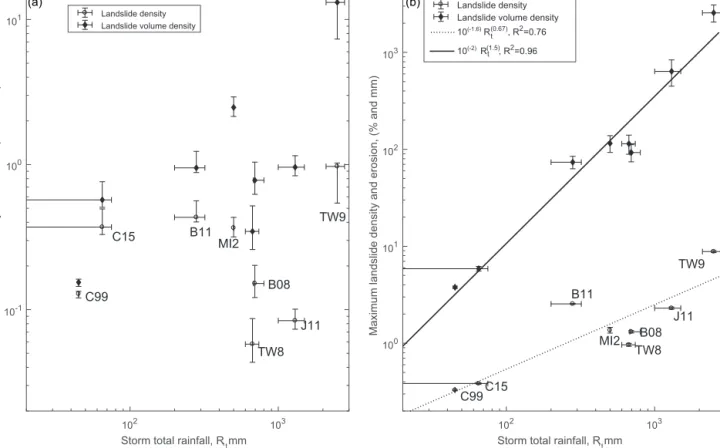
3.2.2 Maximum and mean landslide density
Understanding what controls landslide density is a key ob-jective to better constrain hazards and their consequences. For each storm, we compute the mean landslide density (in area and volume) by dividing total landsliding by the land-slide distribution area (Fig. 6a). This density represents the whole affected area and hides important spatial variability (Fig. 1), thus we also compute the maximum landslide
den-0 10 20 30 40 50 60 70
Slope gradient, degree
0 0.01 0.02 0.03 0.04 0.05 0.06 0.07
Probability density function
-10 0 10 20 30 40 50
Slope gradient minus topographic modal slope, S-S ,, degree M
10-1 100 101
Probability ratio (landslide/topography)
C99 B08 C15 B11 MI2 TW8 TW9 J11 ChiChi (a) (b)
Figure 4.(a) Slope gradient probability distribution for the affected topography (solid) and the landslide scar areas only (dashed), for the eight rainfall events and as a comparison to the Chi-Chi earthquake. (b) Ratio of the two probability distributions against the difference
between slope gradient and the modal topography. The ratios are estimated with the PDF averaged within 3◦bins. Solid circles and dots
represent ratios where the landslide probability is beyond or within, respectively, the 95 % prediction interval of the topography distribution. Crosses indicate bins where data are insufficient for the validity of the central limit theorem required to estimate prediction interval.
sity by computing the total landsliding (again in area and vol-ume) within a moving window of 0.05◦(∼ 25 km2), assign-ing landslides to a cell based on their centroid locations and selecting the maximal value (Fig. 6b). Given the better corre-lation obtained above with a run-out normalization, we focus on area and volume densities derived from scar estimates.
The mean landslide densities vary between 0.01 %–1 % and 100–10 000 m3km−2but with poor correlation with to-tal rainfall (R2=0.01 and R2=0.46 for area and volume density, respectively). Indeed, given that both total landslid-ing and distribution area increase strongly with total rainfall, their ratio is relatively independent. In contrast, the maxi-mum landslide scar density and volume density range from 0.1 % to 5 % and 0.002 to 1.5 millions m3km−2 , respec-tively, and are strongly correlated with a power-law of total rainfall (R2=0.76 and R2=0.95). We found very similar correlations when computing the local density on a grid of 0.03 or 0.1◦, but degraded correlations when using the whole landslide area to compute landslide density (R2=0.40 and R2=0.69). We also note that, as for the total landsliding, maximum landslide density and volume density are signifi-cantly correlated with peak rainfall intensity, I 3 (R2=0.58 and R2=0.67, respectively), and duration, D (R2=0.70 and R2=0.73, respectively), although less strongly than with total rainfall.
3.2.3 Landslide size, run out, and position on slope
The decay exponents of the distribution of landslide area do not correlate significantly with any storm metrics (intensity, duration, or total rainfall; |R| < 0.1). However, after run-out normalization, the decay exponents of landslide scar area correlate with all metrics, although with significant scatter (R2∼0.5 Figs. 3, 7). The two largest storms (J11 and TW9) have the lowest exponents (α + 1 ∼ 1.8), and thus a large proportion of very large landslides, while the two smallest storms (C15 and C99) have a small proportion of large land-slides and large exponents (α + 1 ∼ 2.7). However, interme-diate cases are very scattered, as B11 and TW8 have sim-ilar total rainfall, peak intensity, and duration but very dif-ferent distribution with α + 1 = 1.9 and with α + 1 = 2.6 , respectively. Still, randomly removing one event (i.e., jack-knife sampling) we obtained R2between 0.4 and 0.7, with a similar mean R2of about 0.5.
The decay exponents of the equivalent aspect ratio (Figs. 3, S6) do not correlate significantly with any storm metrics (intensity, duration, or total rainfall; |R| < 0.2). In-deed, long run-out landslides are abundant for the smallest storms, C99 and C15, as well as for the second largest storm, J11, but are relatively rare for other storms (e.g., MI2,TW8, B08), spanning the whole range of storm indexes. Similarly, the mean and modal aspect ratio are similar for all events
Figure 5.Total landsliding in area and volume derived from whole landslides (a) or from scar estimates only (b), total landslide number (c) and landslide distribution area (d) against storm total rainfall. M98 is for Mitch 1998. Horizontal error bars show a range of maximum storm rainfall when available (cf., Table 1). In (a) and (b) 1σ uncertainty in the total volumes and areas, ignoring potential landslide mis-detections (cf. methods), are smaller than the symbols (< 10 %). Vertical error bars are based on the range of affected areas in (d), while we could not obtain quantitative uncertainties in the total number (c).
across all storm metrics, except for C99 which is heavily dominated by debris flow and has a modal aspect ratio > 10. We have observed that almost the eight events behave sim-ilarly with respect to the distribution of topographic slopes, not suggesting a strong link with the individual storm proper-ties. The C99 event has a different behavior that may relate to the fact that it was the shortest storm with the smallest total, or that it was the only case occurring in high-elevation terrain with sparse vegetation. C15, the second shortest and smallest storm event may also have strong oversampling about 20◦ be-yond SMbut the limited number of landslides does not allow
us to confirm the significance of this oversampling.
4 Discussion
4.1 Scaling between rainfall and landsliding
We found that total landsliding, peak landslide density, and the distribution area of landsliding were all best described as increasing as a power-law or exponential function of the total storm rainfall, Rt. Our mechanistic understanding of
lands-liding predicts that, for a given site, the mechanism leading to failure is the reduction of the normal load and friction due to the increasing pore-water pressure (Iverson, 2000). This requires progressive saturation of the material above the fail-ure plane and depends directly on the total amount of water poured on the slopes. However, we can envision that land-scapes may rapidly reach an equilibrium in which all un-stable slopes under rainfall conditions frequently occurring would have been removed. In this framework, the rainfall amount relative to the local climate would be more relevant than absolute rainfall, requiring an analysis in terms of devia-tion from the mean rainfall or in terms of rainfall percentiles (e.g., Guzzetti et al., 2008). Although we could not define rainfall percentiles in each area, we note that normalizing Rt
by the mean monthly rainfall relevant for each storm, we still find a decent correlation with the peak landslide density, im-plying climate normalized rainfall variable may be driving landsliding (Fig. S8).
The antecedent rainfall is also expected to play a key role in controlling the saturation level before the triggering storm (e.g., Gabet et al., 2004; Godt et al., 2006). However, if the
102 103
Storm total rainfall, R, mmt
10-1 100 101
Mean landslide density and erosion, (% and mm)
TW8 C99 B08 C15 J11 MI2 TW9 B11 Landslide density Landslide volume density
102 103
Storm total rainfall, R, mmt
100 101 102 103
Maximum landslide density and erosion, (% and mm)
TW8 C99 B08 C15 J11 MI2 TW9 B11 Landslide density Landslide volume density 10(-1.6)R t (0.67), R2=0.76 10(-2)R t (1.5), R2=0.96 (a) (b)
Figure 6.Mean landslide density (a) and peak landslide density in a 0.05◦sliding window (b), against storm total rainfall. Landslide area and volume are derived from scar estimates, i.e., removing run-out contribution. Horizontal error bars show a range of maximum storm rainfall when available (cf., Table 1). Vertical error bars are based on the range of affected area in (a) (the most uncertain term), and represent 1σ uncertainty in the total volume and area density in (b), ignoring potential landslide mis-detections (cf. methods).
regolith is already close to the field capacity, significant parts of antecedent rainfall may be drained from the regolith within some hours or days (Wilson and Wieczorek, 1995), and as a result, the contribution of past storms may be negligible compared to heavy rainfalls over relatively short time inter-vals (1–4 days). However, for moderate storms, like C15 or C99, and especially during dry periods when the slopes are saturated below field capacity, the role of antecedent rain-fall may be more substantial. Thus, we expect that moderate storms happening after prolonged dry or wet periods may de-viate downward or upward from the scaling, respectively. We also note that the abundance of larger and deeper landslides, strongly influencing the total volume or erosion, may depend on deeper water level rather than regolith saturation and thus may be most sensitive to water accumulation over several days rather than a few hours (Van Asch et al., 1999; Uchida et al., 2013). Therefore, although we obtained a good corre-lation without considering antecedent rainfall, its role should be assessed in future refined scalings. Last, the scaling re-ported here is based on events where all landslides occurred within a short time frame (few hours to few days), and would not apply to a monsoon setting where landslides occur more or less continuously during several weeks (Gabet et al., 2004;
Dahal and Hasegawa, 2008), driven by continuous, heavy but unexceptional, rainfall. Indeed, in a long period with fluctu-ating rainfall such as the monsoon, drainage and storage of water will certainly not be negligible and the derivation of a soil water content proxy will be necessary (e.g., Gabet et al., 2004).
The strong correlation between Rt and Ad suggests that
storms able to generate greater amounts of rainfall also tend to deliver a sufficient amount of rain over broader areas. For tropical storms and hurricanes (5 out of 9 cases in Fig. 5d) a number of studies (cf., Jiang et al., 2008, and references therein) found that the maximum inland storm total rainfall (i.e., Rtfor us) correlated well (R > 0.7) with a rainfall
po-tential defined as the product of storm diameter and storm mean rainfall rate within this diameter over storm velocity, each term measured 1–3 days before the storm made land-fall. It was also generally observed that rainfall intensity is higher closer of the storm core, thus potentially tightening the link between Rt and a given storm radius with intense
rainfall and high landslide probability. These observations would imply linear proportionality between Rt and Ad and
could be consistent with the observed power-law trend (ex-ponent 1.5; Fig. 5), especially if some further links between
101 102 103 Storm metrics 1.8 1.9 2 2.1 2.2 2.3 2.4 2.5 2.6 2.7
IGD scaling parameter,
+1 TW8 C99 B08 C15 J11 MI2 TW9 B11 I3, mm h D, h Rt, mm 3.9 R R² = 0.5 -0.09 t -1
Figure 7.Landslide scar size distribution decay exponents against storm total rainfall (red), storm duration (blue) and storm peak intensity (black). The best least-squares fit is shown in red. The reduction of the decay exponents with increasing storm magnitude indicates an increase in the proportion of large landslides relative to small landslides.
Rtand mean storm intensity or velocity exist. Potential links
between Rtand Adfor smaller-scale storms (C99, C15, B08,
and B11) are harder to interpret, and we cannot exclude that it is a coincidence allowed for by our small number of events. In any case, the broader zone is not likely to receive ho-mogeneous rainfall amount, decoupling mean landslide den-sity from storm maximum strength (Fig. 6a). The variability in rainfall within these extended zones is likely a main con-trol on the spatial variability in landslide density, although lithological properties or slope distribution may also matter. Indeed lithological boundaries or a lack of steep slopes can sometimes explain spatial variability in landsliding, but not all of it (e.g., Fig. S9). In any case, it seems clear that to predict the spatial variability of landsliding, the rainfall spa-tiotemporal pattern is a primary requirement. The good cor-relation between storm total rainfall and peak landslide den-sity is encouraging and suggests that, as most mountainous regions may have sparse instrumental coverage, the use of satellite measurements (Ushio et al., 2009; Huffman et al., 2007) or meso-scale meteorological models (e.g., Lafore et al., 1997) may be required to understand the spatial pat-tern of rainfall-induced landsliding.
A few nonlinear scalings between total landsliding and to-tal rainfall have been reported at the catchment scale, but were derived from datasets not easily comparable to the one presented in this study (Reid, 1998; Chen et al., 2013; Marc et al., 2015). The details of this scaling are of importance in
order to understand the impact of extreme rainfall events and more generally which type of rainfall event contributes most to sediment transfer over long timescales (Reid and Page, 2003; Chen et al., 2015). We also found nonlinear scaling be-tween Rtand total landslide area, but without a strong
statis-tical difference between exponential or power-law functions. Exponential functions yield a minimum landsliding amount at low rainfall, that is not physically justified. This appar-ent contradiction may, however, be resolved by considering a rainfall threshold below which landsliding is null. The higher correlation between Rtand total volume is likely due to the
fact that Rt correlates well with maximum landslide size
(R2=0.8 with whole landslides, R2=0.9 and almost linear correlation with scar estimates, Fig. 10), with large landslides contributing most of the total volume and erosion. A correla-tion between Rtand large landslides may arise because
land-slide stability is determined by the ratio between pore pres-sure and the total normal stress on the slip plane, meaning that larger landslides that usually have deeper failure planes (Larsen et al., 2010) may only fail with greater precipitation amount. However, given that the trend between total rainfall and the landslide size distribution is much weaker, this cor-relation may also partly result from a sampling bias as the probability to draw large landslides increases with the total number of landslides. For now, our unreliable estimates of total landslide number do not allow for quantifying this ef-fect.
In any case, several caveats should be taken with the pre-liminary scalings between total storm rainfall and total land-sliding. First, the definition and limit of a single “storm” is not generally agreed in the meteorological community, be-cause the atmospheric fluids suffer perturbations with scale interactions, and therefore with events not independent from each other. Ideally, future studies could categorize storms ac-cording to some space-time filtering and analyze the scalings with total landsliding for each storm category. Currently, our database is not sufficient for this. Second, linking total rain-fall in a limited area and the total landsliding within the storm footprint implicitly suggests that storm rainfall is somewhat structured with internal correlations between peak rainfall, storm size, and the spatial pattern of rainfall intensity within the storm. This seems to be the case for large tropical storms (Jiang et al., 2008), but should be explored for a broader range of storm types. Orographic effects (e.g., Houze, 2012; Taniguchi et al., 2013), focussing high-intensity rainfall on topographic barriers, may also enhance such a correlation between local total rainfall and the broader pattern of rain-fall and landsliding. Last, the scaling with rainrain-fall may also be obscured by outliers due to processes not controlled by rainfall. For example, the inclusion of the very long run-out components in several inventories led to larger scattering for both power-law and exponential models and to favor the lat-ter. Therefore, the proposed run-out correction seems essen-tial for future studies. Another issue concerns the normal-ization of landscape parameters affecting the susceptibility to landsliding, such as hillslope steepness and mechanical strength (Schmidt and Montgomery, 1995; Parise and Jib-son, 2000; Marc et al., 2016). Nevertheless, the proportion of flat or submerged land within the area of the most intense rainfall must limit the total landsliding, as it was certainly the case for MI2 or B08 (Fig. 1). Recent, widespread an-tecedent landsliding may also reduce subsequent susceptibil-ity to rainfall triggered by removing the weak layer of soil or regolith on steep slopes. In the pre-event imagery, we did not see specific evidence of such a limitation, except maybe for J11, where abundant pre-event fresh landsliding were visible near 136,25◦E/34,29◦N and 135,9◦E/34,20◦and very few new landslides occurred. A more systematic evaluation of this effect may be important when quantitatively comparing the landslide and rainfall patterns. In any case, it is clear that further analysis of this database, possibly extended with ad-ditional landslide inventories, should be used by future stud-ies to refine the scaling with rainfall and incorporate the ef-fects of controlling parameters such as available topography, antecedent rainfall or regolith properties (e.g., strength and permeability).
4.2 Relation between rainfall and landslide properties
We found an increase in the proportion of large landslide scars with all storm metrics, but clearest with the total rain-storm (Fig. 7). This is consistent with the idea that large
landslides require larger amounts of rainfall to be triggered (Van Asch et al., 1999), as discussed above and exemplified with the strong correlation between Rt and maximal
land-slide scar (Fig. S10). The large remaining scatter suggests that other differences between the inventories matter, such as differences in the mechanical properties of the substrate (e.g., Stark and Guzzetti, 2009). Indeed, broad lithological contrast exists between each event, and sometimes within an event (Fig. S9). The variability in extent and thickness of weak su-perficial layers (i.e., soils) between the different landscapes affected may also be important. Variations in slope distribu-tion and relief are also wide between each case (Figs. 1, 4) and have also been reported to influence landslide size (Frat-tini and Crosta, 2013).
We note that the positive correlation between peak rainfall intensity and large landslide abundance is opposed to what could be expected, as more small landslides are expected for pulses of very intense rain leading to the occurrence of tran-sient high pore-water pressure pulses at shallow depth (Iver-son, 2000). Given that water retention and hydraulic conduc-tivity may easily change by orders of magnitude between dif-ferent environments, it may be needed to normalize intensity by the regolith hydraulic conductivity (Iverson, 2000) to un-derstand its potential influence. For the moment, we consider that the correlation between D and I 3 and the landslide size distribution exponents likely arises because of the correlation between these storm metrics and Rt(Fig. S4)
In any case, our results suggest that it is not only the landscape properties that set the landslide size distribution but also the trigger characteristics, as previously reported for earthquake-induced landslide size distributions (Marc et al., 2016). This means, for example, that the influence of forcing variability should be assessed and normalized before invert-ing landslide size distribution parameters to obtain regional variations of mechanical properties (e.g., Gallen et al., 2015). In contrast, aspect ratio or run out did not correlate well with storm metrics and thus obscured any direct correlation between storm metrics and the decay exponents of whole landslide area. This underlines again the importance to iso-late scar geometry to deconvolve processes driving landslide initiation and landslide run out. As for the landslide size distribution, landslide run out may likely be influenced by slope and relief distributions, as well as by hydrologic pro-cesses. The case of C99, with exceptional run out for most of its landslides is interpreted as the effect of low infiltra-tion rates favoring large runoff generainfiltra-tion (Godt and Coe, 2007). This may also explain the abundance of debris flow in other places (C15, J11) but cannot be verified without in-formation on infiltration rate in these places to normalize the intensity variations. An alternative could be to study various storms occurring over the same region, and where infiltration rate or conductivity could be assumed constant; for example, with datasets from multiple typhoons in Taiwan (Chen et al., 2013).