Domino Tiling, Gene Recognition, and Mice
by
Lior Samuel Pachter
B.S. in Mathematics
California Institute of Technology (1994)
Submitted to the Department of Mathematics
in partial fulfillment of the requirements for the degree of
Doctor of Philosophy
at the
MASSACHUSETTS INSTITUTE OF TECHNOLOGY
June 1999
©
Lior Pachter, MCMXCIX. All rights reserved.
The author hereby grants to MIT permission to reproduce and
distribute publicly paper and electronic copies of this thesis document
in whole or in part, and to grant others the right to do so.
A uth or ...
Department of Mathematics
May 4, 1999
Certified by ... ... .. ...
Bonnie A. Berger
Associate Professor of Applied Mathematics
Thesis Supervisor
Accepted by ...
...
Michael Sipser
Chairman, Applied Mathematics
Committee
Accepted by .
...
INSTITUTE
Richard Melrose
Domino Tiling, Gene Recognition, and Mice
by
Lior Samuel Pachter
Submitted to the Department of Mathematics on May 17, 1999, in partial fulfillment of the
requirements for the degree of Doctor of Philosophy
Abstract
The first part of this thesis outlines the details of a computational program to identify genes and their coding regions in human DNA. Our main result is a new algorithm for identifying genes based on comparisons between orthologous human and mouse genes. Using our new technique we are able to improve on the current best gene recognition results. Testing on a collection of 117 genes for which we have human and mouse orthologs, we find that we predict 84% of the coding exons in genes correctly on both ends. Our nucleotide sensitivity and specificity is 95% and 98% respectively.
Most importantly, our algorithms are applicable to large scale annotation prob-lems. The methods are completely scalable. We are able to take into account multiple or incomplete genes in a genomic region, splice sites without the usual GT/AG con-sensus, as well as genes on either strand. In addition to our algorithmic results, we also detail a number of computational studies relevant to the biological phenomena associated with splicing. We discuss the implications of directionality in splice site detection, statistical characteristics of splice sites and exons, as well as how to apply this information to the gene recognition problem.
The second part of the thesis is devoted to combinatorial problems that originate from domino tiling questions. Our main results are upper and lower bounds for forcing numbers of matchings on square grids, as well as the first combinatorial proof that the number of domino tilings of a 2n x 2n square grid is of the form 2n(2k + 1)2. Our approach to both problems is concrete and combinatorial, relying on the same set of tools and techniques. We also discuss a number of new problems and conjectures. Thesis Supervisor: Bonnie A. Berger
Acknowledgments
I thank my mom and dad first, not that "thanks" can express my gratitude for what
they have contributed to me. I hope that the readers of this thesis can know what I mean.
The work described herein is the result of, and epitome of, collaborative research.
I am deeply indebted and grateful to all who worked with me on the various aspects
of what has become a thesis.
The guidance and thoughts of my advisor, professor Bonnie Berger, are evident throughout my work. I thank her for her help and for the unwavering support I re-ceived during my studies. I am grateful to professor Daniel Kleitman for suggesting the use of dictionaries in gene recognition, and for the many contributions he made during the ensuing developments. The key idea of applying comparative genomics principles to gene recognition was suggested by professor Eric Lander, who subse-quently contributed many excellent ideas in critical moments. Above all, I thank Serafim Batzoglou who has been my colleague and friend for the last two years. His contributions and efforts directly enabled the completion of much of the gene recog-nition project described in this thesis. My thanks also go to Val Spitkovsky, who created and developed the dictionary described in Chapter 5. Eric Banks, Bill Wallis, Theodore Tonchev and John Dunagan, all contributed, both by coding and thinking, in countless ways to the research I did. Thank you all.
Of course, I cannot omit my thanks to those who turned my love affair with
math-ematics into a marriage. I thank my father for showing me what mathmath-ematics is, my friend and mentor Nitu Kitchloo for helping me realize that I can be a mathematician, professor Daniel Kleitman for showing me how to be one, and my students through-out the years for giving me a reason to continue being one. Special thanks go to my mother who taught me about those things in life that are much more important than mathematics. There have been many others who have inspired me and taught me, and of course along with those mentioned above, they all deserve much more than a thank you note in my thesis.
The influence and help of all of my friends is evident throughout this thesis. Fortu-nately, I have too many friends to list. Still, I cannot resist the temptation to specially thank Dave Amundsen (I did beat him at pigskin), Dave Finberg (the computer and combinatorics stud), Jing Li (thanks for the angst), Nitu Kitchloo (brother), Tal Malkin (vodka madame?), Mats Nigam (thanks Linda!), Boris Schlittgen (see Jing Li) and Glenn Tesler (who TeXed most of the difficult stuff in this thesis).
Thanks to Beth Hardesty for ungrouching me many times, often during critical moments of my graduate student career. Finally, I'd like to thank my love Son Preminger for all her help, understanding and fanchuking.
Contents
N otation . . . .
I
Gene Recognition
Overview . . . .
1 Biology Background and Goals 1.1 The Genetic Dogma ... 1.2 The Splicing Cycle ...
1.3 Biological Signals and Patterns in DNA . . . .
1.4 What do you do with 100KB of human genomic DNA
1.5 The Computational Challenges in Gene Annotation .
1.5.1 Exon Prediction . . . .
1.5.2 Other Problems . . . .
2 Previous Work on Gene Annotation
2.1 Similarity Searching and Gene Annotation . . . . 2.2 Statistical Approaches . . . .
2.3 Homology Approaches . . . .
2.4 H ybrids . . . .
2.5 R esults . . . . 3 Identification of Introns and Exons
3.1 Splice Sites . . . .
3.1.1 Pairwise Correlations . . . .
3.1.2 The GENSCAN splice site detector . . . .
3.1.3 Left Rules . . . .
3.2 Introns ... .. ... . ....
3.2.1 Length Distribution . . . .
3.2.2 Pair Correlations in Introns . . . .
3.2.3 G+C effects . . . .
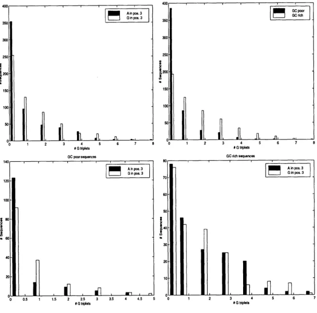
3.2.4 G triplets near the donor splice site . . . .
3.3 Exons ... ... ...
3.3.1 Length Distribution . . . .
3.3.2 Pair Correlations in Exons . . . .
3.3.3 The Frame . . . . 13 15 . . . . 16 17 17 19 20 25 25 26 26 28 28 29 29 29 30 32 . . . . 32 . . . . 32 . . . . 35 . . . . 36 .. ... 38 . . . . 42 . . . . 42 . . . . 43 . . . . 44 . ... . 45 . . . . 45 . . . . 47 . . . . 47
4 Assembling a Parse 55
4.1 Introduction . . . . 55
4.2 Complexity of the Problem . . . . 55
4.2.1 A visit with Fibonacci . . . . 55
4.2.2 Average case analysis . . . . 56
4.2.3 Mitigating factors . . . . 57
4.3 A Dynamic Programming Approach . . . . 57
4.3.1 General Framework . . . . 57
4.3.2 Frame Consistent Dynamic Programming . . . . 58
4.3.3 Technical Issues . . . . 58
5 Dictionary Approaches 60 5.1 Introduction . . . . 60
5.2 M ethods . . . . 61
5.2.1 Dictionary Lookups and Fragment Matching . . . . 61
5.2.2 Dynamic Programming . . . . 63
5.3 Results and Discussion . . . . 63
5.3.1 Output of the Program . . . . 63
5.3.2 Alternative Splice Sites . . . . 64
5.3.3 Exon Prediction . . . . 66 5.3.4 Other Applications . . . . 68 5.3.5 Discussion . . . . 69 5.3.6 Running Times . . . . 70 6 Comparative Genomics 72 6.1 Introduction . . . . 72
6.1.1 The Rosetta Stone . . . . 72
6.1.2 A New Paradigm for Gene Annotation . . . . 73
6.2 Alignments . . . . 74
6.2.1 Background . . . . 74
6.2.2 Nested Alignments . . . . 75
6.3 Finding Coding Exons . . . . 77
6.3.1 Removing Regions with Bad Alignment . . . . 77
6.3.2 Scoring a Pair of Exons. . . . . 78
6.3.3 Piecing together Exons . . . . 80
6.4 R esults . . . . 80 6.5 D iscussion . . . . 82
II
Combinatorics
103
O verview . . . . 104 7 Forcing Matchings 105 7.1 Introduction . . . . 105 7.2 Preliminaries . . . . 1057.3 The Upper Bound . . . . 106
7.4 The Lower Bound . . . . 108
7.5 A Min Max Theorem ... 110
7.6 Other Problems ... ... 112
8 Tilings of Grids and Power of 2 Conjectures 113 8.1 Introduction . . . . 113
8.2 The square grid . . . . 114
8.2.1 Even Squares . . . . 114 8.2.2 Odd Squares . . . . 119 8.3 Rectangular Grids . . . . 123 8.3.1 2 x n grids . . . . 123 8.3.2 n x m grids . . . . 128 8.4 Conjectures . . . . 128
8.4.1 Deleting From Diagonals . . . . 128
8.4.2 Deleting From Step Diagonals . . . . 129
8.5 D iscussion . . . . 131
A Biology Tables 132 B Datasets 137 B.1 Description of the Databases . . . . 137
B.1.1 Learning . . . . 137
B .1.2 Testing . . . . 138
B .2 Tables . . . . 138
List of Tables
1.1 Assumptions about the DNA in which one is to find coding exons . 26
2.1 Accuracy statistics for programs on the BG dataset . . . . 30
3.1 X 2 values for the (-3,5) donor window. . . . . 35
3.2 The correlation coefficient for GC content between an intron (exon) and its neighboring introns and exons. . . . . 43
3.3 GC content and the number of G triplets. . . . . 44
3.4 The Best Frametests . . . . 52
5.1 OWL hits returned with a minimum length cutoff of k = 8 amino acids. 65 5.2 Genes from the Burset-Guig6 database with exons expressed in two frames. Unless otherwise specified, the genes are human. . . . . 67
5.3 Statistics for the OWL protein database. . . . . 68
6.1 Summary of results for all coding exons. . . . . 81
6.2 Summary of results for interior coding exons. . . . . 82
6.3 Summary of results for exterior coding exons. . . . . 82
6.4 Analysis of alignments and results on the HUMCOMP/MUSCOMP test set... ... 97
6.5 Results with the multiple genes assumption, parsed in pieces. . . . . . 98
6.6 Results with the parsed in pieces assumption. . . . . 99
6.7 Results with the multiple gene assumption and double strand assumption 100 6.8 Results with the single gene assumption. . . . . 101
6.9 GENSCAN results on the HUMCOMP dataset . . . . 102
A.1 The Genetic Code . . . . 132
A.2 The PAM20 matrix. . . . . 134
A.3 Codon Usage in Humans . . . . 135
A.4 Codon Usage in Mice . . . . 136
B.1 The HUMCOMP/MUSCOMP Datasets . . . . 178
B.2 The HKRM dataset . . . . 179
B.3 The BG dataset, part 1 . . . . 180
B.4 The BG dataset, part 2 . . . . 181
B.5 The BG dataset, part 3 . . . . 182
C.1 Values of S(n, k) for n = {2,...,6}, k < [IJ . . . . 184
C.2 Number of tilings of the 2n x 2n square grid with k edges removed
from the lower left corner . . . . 184
C.3 Number of tilings of the 2n x 2n square grid with the rth edge removed
from the step-diagonal . . . . 185
C.4 Number of tilings of a (2n + 1) x (2n + 1) square grid with one square removed from the border . . . . 185
List of Figures
1-1 A schematic view of the transcription-translation process. . . . .
1-2 The Splicing Cycle . . . .
1-3 Some of the snRNPs and their interactions . . . .
3-1 Correlation Matrices for donor and acceptor splice sites . . . .
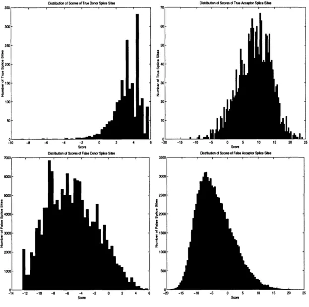
3-2 Scores of True/False Donor and Acceptor Splice Sites . . . . 3-3 Left/Right effects for donor splice sites . . . .
3-4 Left/Right effects for acceptor splice sites . . . .
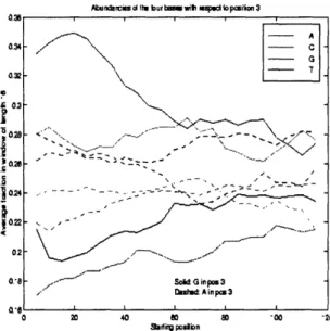
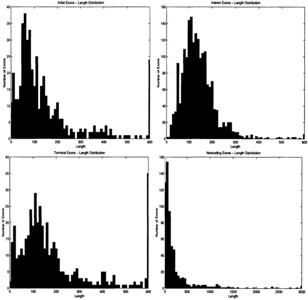
3-5 Scores of True/False Donor and Acceptor Splice Sites with the Left Rule 3-6 Length distribution of introns . . . . 3-7 The effect of the nucleotide in the third position an bases downstream 3-8 G triplets, GC content and Position 3 . . . . 3-9 GC content and Position 3 . . . . 3-10 Length distributions of coding and noncoding exons in genes with
mul-tiple exons . . . .
3-11 Length distributions of simulated exons in multiple exon genes . . . .
3-12 Length distributions of true and simulated exons in single exon genes 3-13 Fram e Prediction . . . .
3-14 Separations for the different Frametests . . . . 4-1 The reason for frame consistent dynamic programming . . . .
Java applet display . . . . The Id3 gene. . . . . An alternative form of the Id3 gene. . . . . .
A difficult alignment problem. . . . .
The Rosetta stone. . . . . The gadd45 gene . . . . Alignment statistics in coding exons . . . . . Alignment statistics outside of coding exons Forced tiling (upper bound) . . . . The bijection . . . . Forced tiling (lower bound) . . . .
. . . . 6 4 . . . . 6 6 . . . . 6 6 . . . . 7 0 . . . . 7 3 . . . . 8 3 . . . . 8 5 . . . . 8 5 . . . . 10 7 . . . . 10 8 . . . . 10 9
7-4 The square grid with its axis of symmetry and labelled diagonal
18 21 22 34 37 39 40 41 42 45 46 47 48 49 50 52 54 58 5-1 5-2 5-3 5-4 6-1 6-2 6-3 6-4 7-1 7-2 7-3 109
Labeling of the diagonal . . . . The grids H. . . . .
A reduced configuration . . . .
An Odd Square with a corner removed The grids S . . . ..
The grids D . . . ..
The (5,2) spider . . . . Tiles on the step-diagonal . . . .
8-1 8-2 8-3 8-4 8-5 8-6 8-7 8-8 115 116 117 120 121 122 129 130 . . . . . . . . . . . . . . . . . . . . . . . . . . . . . . . .
Notation
/
Acronyms
Symbol Description Page
bp base pair
CDS coding sequence, abbreviation used in GENBANK 138 ISI the length of a string of open and closed brackets 56
F, the nth Fibonacci number 56
MMG global alignment algorithm
MMGG global alignment algorithm with gap penalties
PARTIALALIGN alignment algorithm for pieces of sequences
GLOBALALIGN the nested alignments algorithm
MMGGE the alignment score for an exon pair
ma score for a match in an alignment algorithm
mS score for a mismatch in an alignment algorithm g score for a gap in an alignment algorithm
PAM(a, b) the PAM matrix score for a pair of codons a,b
CODONh(a) the log odds ratio for codon a in human sequence
CODONm(a) the log odds ratio for codon a in mouse sequence
Sn Sensitivity
Sp Specificity
AC Aprroximate Correlation
G C H G is an induced subgraph of H
V(G) vertex set of a graph G
E(G) edge set of a graph G
K the complete graph on n vertices
Kn,m the complete bipartite graph
P, the path on n vertices
Rn Rn = P2n ) P2n (2n x 2n rectangular grid) C, the cycle on n vertices
T. Tn = C2n C2 n (torus)
Q,
the n dimensional hypercube (K2E
...E K2 n times)
N(n, m) number of tilings of an n x m rectangular grid 113
N(n, m) same as N(n, m) with one border square removed 119
p(M) forcing number of a matching M 105
c(M) maximum number of disjoint, alternating cycles in M 106
#
R number of domino tilings of a region R 114Nucleic Acid Codes (IUPAC)
Code Bases Mnemonic
A C G T (or U) R Y S W K M B D H V N (or X) A C G T A or G C or T G or C A or T G or T A or C C or G or T A or G or T A or C or T A or C or G any base gap A-denine C-ytosine G-uanine
T-hymine (or U-racil) pu-R-ine p-Y-rimidine S-trong (3 H-bonds) W-eak (2 H-bonds) K-eto a-M-ino not A not C not G not T or U
Part I
Overview
This first part of this thesis outlines the results of an investigation undertaken to identify and annotate genes in human DNA. Even though most of the work described was initiated with this goal in mind, many of the results obtained are of independent biological interest.
We begin in Chapter 1 by reviewing the relevant biology. Much of the discussion is simplified so that the introduction is accessible to persons not familiar with biology (specifically, mathematicians). Additional information may be found in books by Lodish et al., Watson et al. [58, 89], or Lander & Waterman [56]. Readers not familiar with biology jargon might find the glossary by Rieger et al. [73] to be a useful reference. We then proceed to outline the issues and problems addressed in this thesis. We discuss both the overall goals of gene annotation, as well as the particular aspects of various subproblems such as splice site recognition.
Chapter 2 contains a survey of previous related work.
In Chapter 3 we discuss distinguishing features of introns and exons that we dis-covered computationally. We survey some well known characteristics (e.g. length distributions), and also present some new results of our own. In particular, we de-scribe a new statistical technique for distinguishing introns and exons based on frame preference, as well as novel methods for splice site prediction. Our splice site tech-niques are applied in subsequent chapters for the purpose of exon prediction.
Chapter 4 presents the framework of our gene recognition program. We describe our use of dynamic programming as a basic framework within which to do gene recognition. The various statistical tests and computational techniques we describe in the subsequent chapters are integrated within the dynamic programming framework to find "optimal" solutions to the various problems we address.
The "dictionary approach" described in Chapter 5 is an efficient way to score exons in a dynamic programming. It is based on finding matches of an input sequence to sequences in a database.
Chapter 6 describes an intriguing new approach to gene recognition based on an analogy of the Rosetta stone deciphering idea. Instead of using computational tech-niques to predict biological signals in one organism alone, information from another organism is used simultaneously with the first to enhance the signals. The motiva-tion behind this approach is the observed fact that mouse genomic sequence exhibits high similarity to human genomic sequence in coding exons, but this similarity is less apparent in introns and other noncoding regions. We begin by describing a new alignment procedure designed for aligning large genomic regions from the human and mouse. The alignment algorithm represents a breakthrough over previous approaches in speed and accuracy. For example, we show how to align entire 400kB BACs in minutes. We then proceed to show how a good alignment can be used to find coding exons in genes by looking simultaneously at human and mouse aligning fragments. The approach once again uses dynamic programming, as well as many of the same ingredients used in the dictionary approach in Chapter 5; however, the combination of signals in the human and mouse allows for much more accurate predictions.
Chapter 1
Biology Background and Goals
1.1
The Genetic Dogma
The field of biology has been rapidly changing during the past century, largely due to remarkable discoveries in molecular biology. Perhaps more important than the many significant contributions that have been made, is the collective understanding that there is a framework underlying all of biology. The foundation of this framework is made of genes that form the blueprints for a massively parallel, self regulating, dynamical system. This system is incredibly complex, but despite this fact biologists have started to understand it in considerable detail, and one of the principles that have been discovered is that of the genetic dogma. This has been an understanding of how the system operates on a large scale. This chapter is intended to introduce the reader to some of the biology and terminology that is used throughout this thesis. Readers with only a mathematical background will find it useful to refer to more general texts such as Lodish et al. [58], or introductory chapters on biology (written for mathematicians) such as Chapter 1 in Lander & Waterman [56].
For the purposes of our discussion, we will define a gene (see Figure 1-1) to be a single, contiguous region of genomic DNA that encodes for one protein (it will be convenient to also consider the flanking regions that contain promoter signals, etc. as also being part of the gene). There are four different nucleotides that make up a sequence of DNA. These are Adenine (A), Cytosine (C), Guanine (G) and Thymine (T). For our purposes, we will think of DNA as being a string on an alphabet of size 4 (A,C,G,T). DNA physically exists in the form of a double helix (containing two strands, and a gene can be a subsequence occurring on either strand. When a gene is expressed, it is first copied in a process known as transcription. This forms a product known as RNA, which is a working template from which a protein is produced in a process known as translation. Before translation, the RNA undergoes a splicing operation [79] conducted by certain enzymes, which typically delete most
of it, leaving certain blocks of the original strand of RNA intact. These blocks are
called exons and the parts that are removed are called introns. The result of this pruning is the "mature" RNA (mRNA), which is used during translation to make the protein. The protein consists of a sequence of amino acids linked together. During
DNA
5'. TranscriptionRNA
5, .... AGACGAGATAAATCGATTACAGTCA ... 3' - - - AGACGAG UCGAUUACAGUCA ... TranslationProtein
....-
DEI-" Protein Folding Problem SplicingExon Intron Exon Intron Exon
Protein
Figure 1-1: A schematic view of the transcription-translation process.
During translation the T nucleotide becomes a U (Uracil). In this example, the boxed UAA triplet is not a codon and therefore does not end translation. Rather,
the in-frame codons are "...GAC GAG AUA...". These are translated into "...D E
I..." (D=Aspartic Acid, E=Glutamic acid, I=Isoleucine). Splicing occurs before
translation, each amino acid is produced by a triplet of consecutive nucleotides, known as a codon, according to a known map that is called the genetic code (see Table
A.1). This defines the coding frame of the gene.
The gene actually has a "start" translation signal (ATG) and a stop translation sequence (TAA, TAG or TGA) both within exons; the sequence within exons between these forms the coding part of the sequence which contains all the information used to make the protein. The rest of the gene consists of introns, initial and final "non-coding exons" (these are exons that are glued together with the "non-coding exons, but that are not used for making protein), as well as flanking regions containing biological signals of various sorts. Notice that a gene has directionality; it can appear either on the forward direction, or in opposite strand in which case it is traversed in the opposite direction, hence reverse complement. The directionality of a gene is always annotated as 5' -+ 3', that is, the gene is traversed from the 5' to the 3'
direction. The splice sites on the 5' end of an intron are known as donor splice sites. On the 3' end they are known as acceptor splice sites.
1.2
The Splicing Cycle
The mechanism by which introns are spliced from human genes is not completely understood at this time. Nevertheless, a large number of pieces of the puzzle have been discovered, and while they cannot all be put in place at this time, enough is known to present a general picture of the process.
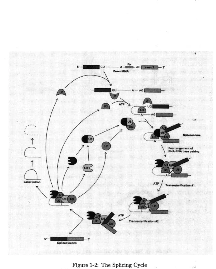
The components responsible for executing various stages of the splicing process are called spliceosomes. These are for the most part RNA-Protein complexes. We discuss some of the more important ones in the following sections, although we em-phasize that it is widely believed at this time that not all the spliceosomes have been discovered. The splicing cycle is summarized in Figure 1-21 in pictorial format.
In order for introns to be properly spliced a number of conditions must be met: There have to be functional splice junction sequences in the pre-mRNA. These are alluded to below, and discussed in more detail in Chapter 3. Secondly, activity of at least three small nuclear ribonucleoprotein particles (abbreviated snRNPs and pronounced "snirps", these are spliceosomes) is required. The critical snRNPs are called U1, U2, U5, U4, and U6 (see Figure 1-3 1). Finally, the presence of ATP is necessary.
Figure 1-2 shows how an intron is excised in a sequence of steps. U1 attaches at the donor splice site by "recognizing" a consensus sequence around the dinucleotide
GT. The recognition is accomplished, in part, by the complementarity of the RNA in
the snRNP to the sequence. The precursor mRNA is cleaved at the 5' site and a lariat (loop) structure is formed between the G at the 5' site and an A further downstream in the intron. This A is part of a small subsequence known as the branchpoint which is recognized by the U2 snRNP. Finally, the 3' exon junction is cleaved and the
'From: MOLECULAR CELL BIOLOGY by Lodish et al. (c) 1986, 1990, 1995 by Scientific
exons are ligated together.
The discussion above omits a number of critical, although contested issues in splicing biology. One of the important issues, is the role of mRNA secondary structure in the spliceosome interactions with the sequence. Evidence in this regard ranges from specific experiments affirming the role of secondary structure (e.g. Coleman and Roesser [19]), to counterarguments based on purely theoretical evidence such as extremely long introns (which would suggest that local structure may not play a large role). The exact role of secondary structure in splicing remains to be determined.
Also, we have ignored some rare and different splicing interactions, where the GT may not be present in the splicing consensus, or other spliceosomes are involved (Sharp &
Burge [80]).
1.3
Biological Signals and Patterns in DNA
The extent and variability of consensus sequences associated with biologically relevant signals largely determine the applicability of the signals for exon prediction. We briefly review the important biology associated with commonly used biological signals, and the consensus sequences associated with them.
Promoters
A Promoter is a DNA sequence that directs RNA polymerase to bind and initiate
specific transcription of genes. Although promoters should, in principle, significantly aid in the distinction of genes (by indicating their exact beginning), the complex nature of the sequences, and their variability, makes the identification of promoters and unsolved problem. In eukaryotes, there is usually a conserved AT-rich region
TATA (known as the Goldberg-Hogness or TATA box). Promoters are not analyzed
in this thesis, in part because their computational recognition is very difficult given the current biology that is known about them. Nevertheless, we acknowledge that future work should, and will, include promoter recognition.
Kozak Consensus
The translation process described in the first section is executed by a ribosome which begins at an initiator codon. The initiator codon is usually ATG (methionine), and is surrounded by a relatively weak consensus known as the Kozak consensus [53]. The Kozak consensus is the sequence CCRCCATGG. ATG is the preferred initiation codon (and appears in all of our learning and test genes), there are exceptions to this "rule". In humans, the codons ATA and ATT also appear as initiation codons and in mice there is also ATC. Because of the rarity of these occurrences, we have not allowed for the possibility of such initiation codons in this thesis, although a careful study of them and their consensus sequences is clearly necessary in future work.
5Gin G - --- -- - -.A- AG
A
Am A */
t La~ot Iitron 8~ 3TFigure 1-2: The Splicing Cycle
m
Plearmn9o"mrst of RNA-RNA bo" poiring
ATP) Transootoificatioo#I, frnetdfcdn# 'Afflkh, Anna A '"Ura is U A -,-, AG
offmo-mOA
-,U 4 kAC U A a Syxyya
AtflCJAAr
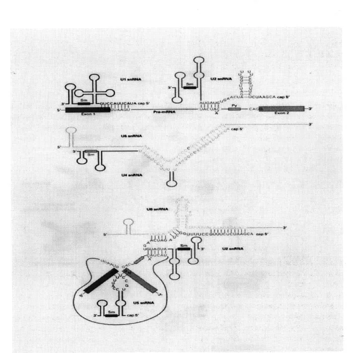
A uA ACA 4rFigure 1-3: Some of the snRNPs and their interactions
The figure shows how the U4 and U6 snRNPs interact with each other, as well as the complex interaction between U2, U5 and U6. U1 is complementary to the consensus sequence CAGGTAAGT at the donor splice site in introns. Notice that the triplet
Signal Peptide
Also known as the leader sequence or signal sequence, this is a region of DNA following the initiation codon that initiates and mediates translocation of membrane and secretory proteins across the cell membrane or endoplasmic reticulum. The region is translated at the beginning of protein synthesis into a polypeptide that is recognized
by protein-RNA complexes (and later cleaved). The region is characterized by a 7-15
long amino acid chain of hydrophobic residues. The cleavage site consists of a more polar C-terminal region.
Splice Sites
Of the many biological signals involved in splicing, the splice sites themselves are
the best studied, and many results have been obtained regarding specific consensus patterns, as well as biologically relevant features in the neighborhoods of the splice sites. The biologically relevant characteristics of splice sites vary greatly between species, in what follows we discuss the specific case of humans:
Donor splice sites are characterized by a strong consensus of GGTRAG. About half the splice sites obey this consensus. The interaction of the U1 snRNP with this splice site is complex, and many results have been obtained about how and why specific sequences deviate from the consensus. Even though the 9 nucleotides adjacent to the GT seem to be the most important in determining an intron's propensity for splicing, the region adjacent to the splice site in the intron (up to 20 basepairs) seems to also play an important role in splice site selection. In particular, as outlined by McCullough and Berget [63], G triplets play an important role in splicing in certain introns. Surely there are many more such biologically important phenomena.
The acceptor splice site exhibits a much smaller consensus than the donor splice site. Indeed, CAG is the most common ending, with the nucleotide after the AG also having some significance. The region immediately preceding the acceptor splice site is known to enhance splicing when it is rich in pyrimidines (the nucleotides C or T). The pyrimidine rich region is usually of length about 20, and is known as the
pyrimidine tract. Branch Points
The branch point or branch site is the site at which the 5' end of the intron
be-comes covalently attached near the 3' end of the intron during splicing. The branch point is usually somewhere between 20-40 basepairs to the left of the acceptor splice site, and often appears right before the pyrimidine tract. The branch point has a strong consensus in yeast, conforming to the specific sequence TACTAAC. In hu-mans, the consensus is much weaker, usually YNYURAY, although of the many variants CTGAC is common.
Poly A Signal
The poly A signal appears after the stop codon of a gene and signifies the site for
the initiation of polyadenylation. Polyadenylation is an mRNA processing event in eukaryotes characterized by the addition of 50 to 250 adenosine residues to the 3' end of the mRNA (known as the poly(A) tail). The poly A signal consists of a pattern of four to six bases of DNA, for example AATAAA. This consensus pattern (and other consensus sequences) at the end of genes can be used for gene identification, however their identification and application is not explored in this thesis.
Repeats
Repeats are repetitive sequences of DNA that occur throughout eukaryotic genomes.
They form approximately 30% of the DNA. Their importance derives from the fact that they are usually not found in coding exons, and therefore their recognition and annotation is of key importance in gene identification. The origin and role of repeats in human DNA is only partially understood, and is the source of much current research (see Smit [81]).
Repetitive DNA sequences can be classified into four main groups:
1. Repeated Genes.
2. Interspersed repetitive sequences.
3. Tandem highly repetitive sequences.
4. Inverted repeat or foldback sequences.
The interspersed repeats fall into two subcategories: short period interspersed repeats (called SINEs), and long interspersed repeats (called LINEs). The SINEs are usually about 300 bp long sequences, are repeated inside longer DNA segments of a few kilobases, and show high variation (e.g. Alu repeats). The LINEs, on the other hand, are long repeats, often more than a few kilobases, that are more homogeneous than their SINE counterparts. Examples include the Li repeat sequences. Tandem repeats
are short sequences of repeated DNA (such as CACACACACA ... ). These may occur
in coding exons, and are also known as low complexity repeats.
The wide variation in types of repeats, as well as the differences in homogeneity between the different classes, makes them very difficult to identify. Indeed, this is an area of ongoing research, and highly specialized packages such as RepeatMasker [97] have been developed for this purpose. In this thesis, we used RepeatMasker to mask repeats, although we also investigated the applications of the dictionary for repeat masking (discussed in Chapter 5).
1.4
What do you do with 100KB of human
ge-nomic DNA?
Recent advances in DNA sequencing technology have led to rapid progress in the Human Genome Project. Within a few years, the entire human genome will be sequenced. The rapid accumulation of data has opened up new possibilities for biol-ogists, while at the same time unprecedented computational challenges have emerged due to the mass of data. The questions of what to do with all the new informa-tion, how to store it, retrieve it, and analyze it, have only begun to be tackled by researchers (for an excellent discussion about these issues see Lander [55]). These problems are distinguished from classical problems in biology, in that their solution requires an understanding not only of biology, but also of mathematics and computer science. Of the many problems, it is clear that the following tasks are of importance:
" Finding genes in large regions of DNA.
" Identifying protein coding regions within these genes.
" Understanding the function of the proteins encoded by the genes.
The important third problem, namely understanding the function of a newly se-quenced gene, requires the solution of the second problem, identification of critical subregions which code for protein. Protein coding regions have different statistical characteristics from noncoding regions, and it is primarily this feature which enables us to distinguish them. An important aspect of work on the problem is the need to characterize these statistical differences and possibly explain their biological under-pinnings.
1.5
The Computational Challenges in Gene
Anno-tation
The computational task we are concerned with is that of determining from an experi-mentally determined sequence of nucleotides, of length on the order of 100,000, where the genes are, and what proteins these genes produce. We may also be interested in further annotations, describing specific features of the genes, such as repetitive regions, or sites of biological significance. This endeavor has three parts, though in practice one handles them together: the first two are determining where each gene is, and determining which parts of its sequence are exons and which are introns. Con-currently, it is necessary to annotate regions in an attempt to find features useful for the first two problems. In this thesis we focus on the problem of distinguishing exons from introns, although along the way we address some of the other annotation issues that arise.
Fortunately, we are not restricted to using only the obvious biological signals avail-able to nature. Of primary importance is the use of repeats, which occur throughout the human genome, but very rarely in coding exons (see biology background above)
Secondly, the codons (and consequently amino acids) that code for protein, are not uniformly distributed, and their distribution differs from the distribution triplets in introns. This can help in distinguishing introns from exons. We can also use informa-tion from other organisms to enhance our signals (Chapter 6). Other restricinforma-tions such as consistency in coding frame between exons greatly reduces the number of possible parses in a given gene. Indeed, even though in principle the number of parses is exponential in the number of potential splice sites identified (Chapter 4), in practice many genes exhibit only a few possible parses after these numerous constraints are introduced.
1.5.1
Exon Prediction
In this section, we suggest a number of alternative definitions of what the exon pre-diction problem constitutes. The range of possible problems one might try to solve, combined with the vast differences in their difficulty, makes the selection of a goal an important issue. Indeed, results can vary greatly with the same test data depending on assumptions that have been made. The following assumptions are ones that may be appropriate in certain contexts:
1. Consists of one complete gene on the forward strand. 2. Consists of multiple complete genes on the forward strand.
3. Consists of multiple complete genes on either strand. 4. May consists of multiple complete genes, perhaps with
partial genes on the ends, on either strand.
Table 1.1: Assumptions about the DNA in which one is to find coding exons
Solutions to the exon prediction problem have tended to concentrate on the model in which one can assume that there is only one complete gene. While this is useful in many cases, the technology by which genes are sequenced results in large genomic fragments which contain all the generalities listed above (in other words one has to assume that there are multiple genes, pseudogenes, etc.) In this thesis we have de-signed solutions based on different assumptions. For example, the dictionary method in Chapter 5 is based on the "one complete gene" assumption, whereas the compar-ative genomics chapter deals with the more general problem.
1.5.2
Other Problems
The exon prediction problem is complicated by a number of biological phenomena, many of which lead to interesting annotation problems in their own right:
Pseudogenes
A pseudogene is defined to be a DNA sequence significantly homologous (75 to 80%)
to a functional gene, which has been altered so as to prevent any normal function. Pseudogenes can be classified into two categories, those that possess all the structural features of a gene (promoters, exons, introns, etc.) but have been mutated so that they are no longer functional (often a result of duplication of a gene and its silencing), and those that lack introns but do have a poly A tail. The latter type are believed to be the result of reverse transcription of mRNA, followed by integration of the resulting cDNA into a chromosomal site. In Chapter 5, we discuss the possibility of detecting reverse transcribed pseudogenes, by finding two adjacent regions in a gene that look like exons, but that cannot be frame consistent unless they have an intron in between them (of length not 0 modulo 3).
Alternative splice sites
Many genes can be spliced into a number of different variants, depending on envi-ronmental or developmental conditions in the gene. Often, alternative splicings lead to diseases or defects in an organism. Alternative splicing happens when a partic-ular splice site can be selected in a different position, or when it is not used at all. Examples are given in Chapter 5.
The presence of an alternative splice site in a gene, renders the exon prediction problem ill-defined. Since there is no "correct" solution to how a gene is parsed, it makes no sense to try an return a predicted answer.
Thus, annotation of possible alternative splice sites is of great importance, espe-cially since they seem to be abundant.
Branchpoints
The weak consensus of branch points in higher eukaryotes was mentioned in the bi-ology background section of this chapter. This weak consensus makes it difficult to annotate branchpoints, or to effectively use them for exon prediction. The computa-tional problem of annotating branchpoints is unsolved.
Chapter 2
Previous Work on Gene
Annotation
Many computational methods have been developed for the purposes of gene annota-tion (Batzoglou et al. [7]). The different approaches that have been undertaken in an attempt to solve the gene recognition problem can be broadly classified as statistical (some may prefer the term AI/learning based) or homology based. In the past few years, the growing abundance of EST (expressed sequence tag) and protein data has resulted in a combination of both approaches being used in newer programs. In what
follows, we attempt to provide a brief summary of the techniques that have been
used in the past so that the reader can place our work in the appropriate context. In particular, we mention that the dictionary approach in Chapter 5 is an attempt to bridge the gap between statistical and homology based approaches. The work in Chapter 6 represents a novel way of tackling the gene recognition problem; we have coined a new term for it, comparative prediction.
2.1
Similarity Searching and Gene Annotation
Of the many applications of computer science in biology, perhaps the most successful
has been the implementation of algorithms for finding similarities between sequences (for a discussion see Waterman [88]). The most widely used program developed for this purpose is BLAST developed by Altschul and others [3, 4], which is an alignment tool. BLAST is often manually applied for the purposes of gene annotation, including exon prediction and repeat finding. Other similarity search approaches include the
FLASH [74] program which is an example of a clever use of a hash table to keep track of
matches and positions of pairs of nucleotides in a database. The resulting information can be used to extract close matches to a given sequence. Nevertheless, neither of these search approaches have been designed for gene annotation.
2.2
Statistical Approaches
The vast number of exon prediction programs in existence precludes the possibil-ity of providing a comprehensive survey without an extended discussion. Our aim here is to merely point out some of the more popular programs. Statistically based programs include GENSCAN [12), GENIE [54], GENEMARK [61], VEIL [36] (all based on hidden Markov models [HMM's]), FGENEH [83] (an integration of various statistical approaches for finding splice sites, exons, etc.), GRAIL [91] (based on neural networks) and GeneParser [82] (based on dynamic programming and neural networks) . Other approaches include language based techniques such as GenLang [25].
These programs have a number of characteristics in common, perhaps the most important being their reliance on a training set (to learn transition probabilities in the case of HMM's, or weights for neural networks). The problem of understanding the implications of this fact and its relationship to the performance of the programs is very difficult due to the relatively small amounts of publicly available data. We briefly discuss this in the results section that follows.
2.3
Homology Approaches
Homology based approaches exploit the fact that protein sequences similar to the expressed sequence of a gene are often in databases. Using such a target, one can successfully identify the coding regions of a gene. The idea is to find the "best" way to parse an input gene so that it best matches the given target after translation. The alignment based PROCRUSTES [28, 86, 64] program represents a very successful implementation of this idea. When a related mammalian protein is available, this program gives 99% accurate predictions and guarantees 100% accurate predictions
37% of the time; however, the user supplies the target protein sequence.
It is important to note that there are a number of current difficulties that arise in the implementation of homology based approaches. The first problem is the iden-tification of good targets. This problem has begun to be addressed (Section 2.4). Additionally, the databases used to find targets were not designed with gene recog-nition as a goal, and so are not easy to use. For example, the cDNA databases are not always properly oriented. The protein databases may contain translated repeats. These are all issues that need to be dealt with when looking for good targets.
2.4
Hybrids
The difficulty of finding good targets for the homology approach is addressed in a recent approach [38]. Specifically, the AAT tool addresses this by automatically using BLAST-like information from protein or EST databases for exon prediction. The INFO program [57] is based on the idea of finding similarity to long stretches of a sequence in
a protein database, and then finding splice sites around these regions. Such programs are becoming more important as the size of protein and EST databases increase.
2.5
Results
The analysis and benchmarking of gene recognition tools has become a science in and of itself. Of the many articles addressing these issues, we mention the excellent surveys of Burset and Guig6 [13, 30]. With the exception of GENSCAN, the non-homology based algorithms are not sufficiently accurate to be relied upon. Accuracy claims range from 60-90 percent per nucleotide, and 30-80 percent per entire exon with exact numbers dependent on who is making the claim. Table 2.1 is from the
GENSCAN website, containing statistics obtained by GENSCAN [11] as well as
Burset-Guig6 [13]. The programs were tested on the Burset-Burset-Guig6 dataset (abbreviated as the BG dataset, see Appendix B). For definitions of the different statistics computed (such as Sensitivity, Specificity, etc.), see [13]:
Accuracy per nucleotide Accuracy per exon
Method Sn Sp AC Sn Sp ME WE GENSCAN 0.93 0.93 0.91 0.78 0.81 0.09 0.05 FGENEH 0.77 0.85 0.78 0.61 0.61 0.15 0.11 GeneID 0.63 0.81 0.67 0.44 0.45 0.28 0.24 GeneParser2 0.66 0.79 0.66 0.35 0.39 0.29 0.17 GenLang 0.72 0.75 0.69 0.50 0.49 0.21 0.21 GRAIL II 0.72 0.84 0.75 0.36 0.41 0.25 0.10 SORFIND 0.71 0.85 0.73 0.42 0.47 0.24 0.14 XPound 0.61 0.82 0.68 0.15 0.17 0.32 0.13
Table 2.1: Accuracy statistics for programs on the BG dataset
These numbers are probably very optimistic compared to the performance ob-served in practice [30]. The alarming aspect of the current state of the field is that these programs perform much worse when tested on new data, namely genes that have been sequenced, whose intron/exon structure is known experimentally. Indeed, on a new sequence set, the programs identified about 1 in 6 genes correctly and completely missed the exons in 25 percent of the sequences. This poor performance is probably due to a number of factors, the most significant of which is that current "learning" takes place on small data sets which are often filled with errors since they have been annotated by the very same programs that are learning from them! Furthermore, the learning sets are often redundant and are not really true representatives of genes in entire genomes.
In practice, those who find genes use a very different approach. They hope that the cDNA or protein (or a good part of these) that are produced by the gene lie in one of the corresponding data bases. They then submit their sequences to BLAST
[3], a program that finds best matches to members of the data base. When it is
possible to match parts of the gene with an entire protein, then one has the answer to the problem, either by examining the alignments by eye, or submitting the matches to a program such as PROCRUSTES [28]. As the databases grow, the likelihood of
good matches to new genes increases. When this approach fails, they turn to the algorithms mentioned, and seek consensus results from them. The process is tedious, time consuming and does not necessarily produce correct results.
Chapter 3
Identification of Introns and Exons
In this chapter we study various characteristics of introns and exons that help us distinguish them from each other. We begin with a detailed analysis of splice sites. These are of special importance in the discrimination of introns and exons because they occur at the boundaries between the two. We then turn examine the various properties of the introns and exons themselves that are of computational importance.3.1
Splice Sites
In this section we begin by describing some computational/statistical analysis of pair correlations around splice sites. These results lead to interesting observations of possible biological significance (see sections 3.2.2, 3.2.3 and 3.2.4). We continue by describing the GENSCAN splice site detector, and our modification of it which we use in Chapters 5 and 6 for exon prediction.
3.1.1
Pairwise Correlations
We begin by defining some terminology which is essential for our study. The position of a nucleotide around the donor splice site of an intron is defined to be the distance (in nucleotides) to the start of the intron (following the convention used in [58]). Negative positions indicate nucleotides in the exon. For example, positions +1 and +2 in an intron are the well conserved GT nucleotides. Position -1 refers to the last nucleotide in the exon, which is usually a G (note: some authors prefer to start the labeling in the intron with 0).
We also define positions around the acceptor splice site in the same way. In this case however positions -2 and -1 refer to the last two nucleotides in the intron. Notice that positions are always defined relative to the donor or acceptor splice sites. For example, in an intron of length 30, position +12 from the donor site and position -19 from the acceptor site represent the same nucleotide.
Correlation Matrices
Given two positions r, t around the donor splice site we constructed a 4 x 4 contingency table based on a set of genes with intron and exon boundaries marked. The rows and columns in the table are labeled with the four bases A, C, G, T. The ijth entry in the table is the number of times base i appeared in position r with base j in position t.
Given such a contingency table, we then computed Cramer's Statistic to test the null hypothesis that the nucleotide in position r is independent of the nucleotide in position t.
Cramer's statistic is derived from Pearson's Chi-Squared test. Let
fi,
be the entry in the ith row and jth column of a contingency table. The ith row sumfi+
is givenby
fi+
= Ej fij and the jth column sumf+
3 is given by f+j = E> fij. Definef
= E_ 4 =1 fij to be the sum of all the entries and let ej =+J+'.
The statisticwe compute is
X2 (fi- eij )2 (3.1)
i=1 j=1 (
and the null hypothesis is rejected if X2 exceeds X2,9 (a is usually taken to be .05).
Pearson's Chi-Squared Test is good in detecting dependencies between positions, however it is not as useful for measuring relative strengths of correlations. For this purpose, we use Cramer's V2 statistic [1], defined for a x b contingency tables by
X2
V2 = x2(3.2)
n min(a - 1, b - 1) where n is the sample size.
Given some window, say from -k to k, around the donor splice site, we computed Cramer's statistic for each pair of positions r, t (-k < r, t < k) (in our case a = b = 4).
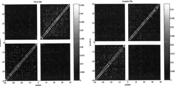
The V2 values were tabulated in a 2k x 2k symmetric matrix which we call the donor
correlation matrix. A similar matrix was also constructed for the acceptor splice
site. Figure 3-1 shows the correlation matrices for donor and acceptor splice sites, computed in for a window of size k = 40.
Observations
It is evident from (3.1) that the diagonal of any correlation matrix is not well defined. We therefore set the diagonal entries to be 0. Similarly, if all the introns in the dataset contain the AG and GT consensus there will be two rows and two columns whose X2 computations contained divisions by 0. Since we only considered splice sites with the
AG, GT consensus, we set the appropriate rows and columns to 0.
Another important trait of our test was the fact that the values in the correlation matrix for a pair of fixed positions depended on the size of the window chosen. This is because introns and exons have finite sizes, so as the window size was increased, the number of introns and exons used in our calculations decreased (for a fixed data set). In addition, since the length distributions of the introns and exons considered
40 -006 40 004 30 0.04 30 . 036 200 003 10 10 0.026 20 10 0.300 000.022 0.025 0.025 -10 -10 0.015 -20 0.1 -20 0.01 -0-30 0.00630OW -4 0 -44 0 0 -4 -30 -20 -10 0 10 20 30 40 -40 -30 -20 -10 0 10 20 30 4
Figure 3-1: Correlation Matrices for donor and acceptor splice sites
changed with window size, we were actually sampling introns and exons with inher-ently different characteristics. We computed tables for a variety of window sizes, but chose to discuss only the k = 40 case in this thesis (and also only the human, as opposed to characteristics in other organisms). More detailed results will appear in follow up work.
As with all Chi-Squared tests for contingency tables, it is important that the values in the contingency table are "sufficiently" large. A commonly used guideline suggested by Cochran [17] is that at least 80 percent of the cells in the contingency table should have counts exceeding 5.0. We observed this to be the case in most of our tests. Nevertheless, for the purposes of our correlation matrices, we decided to use V2 values rather than p-values computed from X2 values. This is because we were more interested in the relative strength of correlations rather in an absolute measure of significance. It can be shown [21] that for an a x b contingency table the X 2 statistic cannot exceed the sample size multiplied by min(a - 1, b - 1). Thus, the V2 statistic provides a good measure of relative associations between datasets although it has no simple probabilistic interpretation.
The pair correlations were studied in terms of their applications to splice site prediction. In particular, the strong correlations between non-adjacent nucleotides close to the splicing site were observed to be the only significant correlations between exons and the introns, and so were examined with regards to possible connections to the splicing process. We mention that similar correlations (computed a bit differently) have recently been analyzed by Burge and Karlin [12].
In Table 3.1 we have listed the X 2 values for the matrix between positions -3 and
5 at the donor splice site (the data is from the -40,40 correlation matrix).
Burge and Karlin [12] provide an interesting analysis of the significance of the correlations, concluding that the absence of base pairings with U1 at certain positions is compensated for by base pairings in other positions. We refer the reader to their
Accoktr Site
0 179 37 0 0 15 38 30 179 0 103 0 0 29 63 70 37 103 0 0 0 12 55 37 0 0 0 0 0 0 0 0 0 0 0 0 0 0 0 0 15 29 12 0 0 0 96 101 38 63 55 0 0 96 0 184 30 70 37 0 0 101 184 0
Table 3.1: X 2 values for the (-3,5) donor window.
paper for a detailed analysis.
The lack of correlation between positions in the intron and the exon away from the splicing site suggest that material in the intron has evolved separately from material in the exon. Indeed, it seems plausible that the intron positions are free to mutate, while the exon positions are constrained by the structural requirements of the protein they code for (this is the basis for the results in Chapter 6). We remark that this lack of correlation can also be used to assist in splice site detection by explicitly measuring (using, say, a X2 test), the lack of correlation between positions in an intron and an
exon.
We decided eventually to settle on a modified form of the splice site detector used in the GENSCAN program [12] (see Section 3.1.3), rather than scoring splice sites based on pair correlations alone. This decision was marginal, since the schemes do not appear to give vastly different results. The GENSCAN splice site detector has the advantage that it gives a score which has a direct, simple, probabilistic interpretation.
In sections 3.2 and 3.3, we present an overview of some other interesting facts and correlations we observed in our human correlation matrices.
3.1.2
The GENSCAN splice site detector
The splice site recognition method outlined in this section is based on the method
by Burge described in [11]. The outline we provide is very vague, the reader should
consult the thesis for exact details.
As an example, we consider the donor splice site detector (the method for the acceptor splice site detector is similar, and we refer the reader to [11] for details). Burge uses a technique he calls Maximal dependence decomposition (MDD). The method generates a decision tree as follows:
1. Calculate for each position i around the splice site, the sum
Si =
Z
x 2(Ci, Xj) (3.3)ii