HAL Id: hal-01780772
https://hal.inria.fr/hal-01780772
Submitted on 27 Apr 2018
HAL is a multi-disciplinary open access
archive for the deposit and dissemination of
sci-entific research documents, whether they are
pub-lished or not. The documents may come from
teaching and research institutions in France or
abroad, or from public or private research centers.
L’archive ouverte pluridisciplinaire HAL, est
destinée au dépôt et à la diffusion de documents
scientifiques de niveau recherche, publiés ou non,
émanant des établissements d’enseignement et de
recherche français ou étrangers, des laboratoires
publics ou privés.
Context Aware MWSN Optimal Redeployment
Strategies for Air Pollution Timely Monitoring
Amjed Belkhiri, Walid Bechkit, Hervé Rivano, Mouloud Koudil
To cite this version:
Amjed Belkhiri, Walid Bechkit, Hervé Rivano, Mouloud Koudil. Context Aware MWSN Optimal
Redeployment Strategies for Air Pollution Timely Monitoring. ICC 2018 - IEEE International
Con-ference on Communications, May 2018, Kansas, United States. pp.1-7, �10.1109/ICC.2018.8422395�.
�hal-01780772�
Context Aware MWSN Optimal Redeployment
Strategies for Air Pollution Timely Monitoring
Amjed Belkhiri
∗†, Walid Bechkit
∗, Herv´e Rivano
∗and Mouloud Koudil
†∗Univ Lyon, Inria, INSA Lyon, CITI, F-69621 Villeurbanne, France †Laboratoire de Methodes de Conception de Systemes (LMCS), ESI, Algiers, Algeria
Abstract—Air pollution has major negative effects on both human health and environment. Thus, air quality monitoring is a main issue in our days. In this paper, we focus on the use of mobile WSN to generate high spatio-temporal resolution air quality maps. We address the sensors’ online redeployment problem and we propose three redeployment models allowing to assess, with high precision, the air pollution concentrations. Unlike most of existing movement assisted deployment strategies based on network generic characteristics such as coverage and connectivity, our approaches take into account air pollution properties and dispersion models to offer an efficient air quality estimation. First, we introduce our proposition of an optimal integer linear program based on air pollution dispersion characteristics to minimize estimation errors. Then, we propose a local iterative integer linear programming model and a heuristic technique that offer a lower execution time with acceptable estimation quality. We evaluate our models in terms of execution time and estimation quality using a real data set of Lyon City in France. Finally, we compare our models’ performances to existing generic redeployment strategies. Results show that our algorithms outperform the existing generic solutions while reducing the maximum estimation error up to 3 times.
Keywords—Air quality monitoring, mobile wireless sensor net-works, WSN redeployment strategies, optimal deployment, error bounded mapping.
I. INTRODUCTION
Air pollution is a major risk on both human health and en-vironment. The World Health Organization report released in September 2016 classified air pollution as the ninth-largest risk on humans with over 7 million premature deaths per year [1]. Moreover, the atmospheric pollution reduces agriculture yields, visibility and sunlight at ground level and increases atmospheric heating as well [2]. These effects highlight the need of a continuous air pollution monitoring and to estimate with a high spatial and temporal granularity the air quality.
The commonly used approach to monitor air pollution is to combine simulations based on fluid mechanics models and measurements of static air pollution stations that provide highly accurate values. However, these stations are very expensive, massive and inflexible which limits their number.
A recent emerging solution for air pollution monitoring consists in the use of Wireless Sensor Network (WSN). The progress of electro-chemical sensors allows to deploy low-cost air pollution monitoring networks with a reasonable cost and high spatial and temporal resolution. Works like [3]–[5] explored WSN-based air pollution monitoring systems and proposed optimal models to reduce deployment costs while ensuring a high precision air pollution estimation. Although these works studied the trade-off between the deployment costs and air pollution assessment precision, they don’t take into account to the dynamic nature of the air pollution dispersion.
WSN movement assisted deployment strategies, or redeployment
approaches are techniques that allow the wireless sensor network to auto-reorganize by relocating sensor nodes to enhance the network performance and the phenomenon coverage [6]. Many WSN deployment strategies have been proposed in the literature. Most of these works rely only on generic definition of network properties such as coverage and connectivity. Unlike these works, we propose context-aware redeployment strategies based on air pollution dispersion model and sensors collaboration in order to generate a high precision air quality map and respond to the dynamic nature of studied phenomenon. To the best of our knowledge, there are no prior similar approaches.
Our proposed models find their application in a wide variety of scenarios such as: pollution monitoring, pipeline leak detec-tion, biochemical attacks, industrial explosions, etc. Using an autonomous swarm of mobile sensors and an adequate rede-ployment approach, such events can be monitored and major risk situations can be avoided. In these applications, static WSN are not suitable for real-time high-resolution monitoring. Thus, highly adaptable, precise and fast strategies are needed. Our main contributions can be summarized as fellows: i) We propose a complete optimal ILP model for WSN online rede-ployment ii) we introduce a hybrid local iterative integer linear program that offers a great compromise between execution time and air pollution estimation quality iii) we present an iterative heuristic algorithm based on local search and taboo list strategies for sensors redeployment in air pollution monitoring application scenario iv) we perform extensive simulations on a real data set to evaluate our models performances and compare them to state of art generic approaches.
II. RELATEDPRIORWORKS
In our work, we are interested in online redeployment strategies that allow to monitor with high precision the air quality. There-fore, we first present prior works that tackled optimal deployment issues. After that, we introduce works relative to mobile WSN redeployment and movement strategies.
A. Optimal deployment strategies
WSN deployment optimization is a very active research area. Several mathematical and algorithmic models are proposed in order to enhance network performances in terms of coverage, connectivity and lifetime. Chakrabarty et al. [7] proposed an optimal 2D/3D grid coverage strategy for target surveillance. They proposed an ILP formulation to minimize the deployment cost and ensure a complete coverage of the deployment region. Other works like [8], [9] used an ILP formulation for multi-objective optimal deployment under connectivity constraints. However, most of these works focus on the network intrin-sic characteristics and they don’t take into account specific application scenarios in which more factors are to consider.
For instance, in air pollution application the common used detection range model for coverage modeling is not suitable, since a physical contact between the pollutant and the electro-chemical sensor is mandatory to determine its concentration in the air. More recently, Boubrima et al. [4], [5] proposed two optimal sensors’ placement models to minimize the deployment cost and to ensure an error bounded pollution estimation. They assumed that sensors don’t have a detection range, instead they used interpolation methods and atmospheric pollution dispersion models to assess pollution concentrations at different points in the deployment region with a bounded estimation error. However, these models don’t consider some properties of the studied phenomenon such as the dynamic nature of the air pollution dispersion, the sudden appearance of new pollution sources and time relative changes in the network. In order to cope with these problems, the use of mobile WSN redeployment strategies is more adequate.
B. WSN redeployment strategies
WSN redeployment is an emerging problem that has been widely studied in the literature. Proposed redeployment strategies are based on different techniques to relocate deployed sensors and to enhance network performances. There are many proposed taxonomies that classify these methods according to different criteria [6], [10].
Among these strategies, we find computational geometric ap-proaches which are based on Voronoi diagram and Delaunay triangulation in order to discover and heal coverage holes in deployment area [11]. Another class of redeployment algorithms is the coverage pattern based strategies, where the network is divided into a virtual grid of predefined pattern according to which sensors are redeployed [12]. We also find virtual forces’ algorithms (VFA). VFA techniques are inspired by the potential field concept from robotics where sensors behave as electromagnetic particles or molecules [13].
Existing ILP strategies focused on optimal static deployment or finding the optimal path for mobile sinks. In contrast, our ILP formulation allow to relocate already deployed sensors to enhance the phenomenon coverage and the network perfor-mances under mobility constraints. Moreover, we base on the intrinsic characteristics of the studied phenomena to define our redeployment strategies.
III.PRELIMINARIES
A. Deployment region and reference map
For all proposed models and without loss of generality, we approximate the deployment region by a 2D virtual grid P of l × w cells. Each cell center p, characterized by its real air pollution concentration Gp and its coordinates (xp, yp),
repre-sents a potential deployment position for a sensor s. The set of real atmospheric pollution concentrations Gp, also known as
ground truth values, at grid points p forms the air pollution concentrations reference map, Rmap= {Gp, p ∈ P}.
B. Simulation map and reference map approximation
In real application scenarios, the construction of the air pollution reference map requires punctual and time continuous measuring at each point p of the deployment region, which is not feasible. Therefore, we rely on atmospheric dispersion simulations that
use physico-chemical models of gas or particle dispersion based on a pollutant emissions, meteorology (temperature, humidity, wind speed,...) and geometry of streets and buildings in order to estimate the concentration of pollutants with a high spatial gran-ularity. These values form the simulation map Smap= {Sp, p ∈
P} that approximates the ground truth map Rmap. For each
point p, the estimated value Sp presents a maximum simulation
error that we call Sep. This maximum error can be estimated
using existing models like [14] and it is usually proportional to the estimated pollution concentration value. Hence Sp and Sep
verify the relation: Sp− Sep≤ Gp ≤ Sp+ Sep.
C. Measurement based estimation and error map
We represent sensors distribution by X, an l × w matrix, where Xp∈ {0, 1} indicates the presence of a sensor at position p.
We denote the measured values by each sensor deployed at position p, Sp. Standard detection region models where we
assume that each sensor has a detection range are not suitable in our context as explained before. Therefore, in order to estimate concentrations where no sensors are deployed and to cope with this limitation, a variety of estimation methods have been proposed in the literature (atmospheric dispersion, land use regression, interpolations..) [15]. In this work, we use a determin-istic spatial interpolation method called IDW (Inverse Distance Weighting). This method formulates the estimated concentration Zpat a given position p where no sensor is present as a weighted
combination of reference concentrations Sqmeasured by sensors
deployed at points q as expressed in formula (1).
Zp= P q∈P−{p}Wpq×Sq P q∈P−{p}Wpq if Xp= 0 Sp if Xp= 1 (1)
Each measured concentration Sq has a weight Wpqcalled
corre-lation coefficient. This coefficient expresses the spatial similarity between p and q as follows:
Wpq= 1 D(p,q)α if q ∈ Ndc(p) − {p} 0 if q /∈ Ndc(p)
Where D(p, q) represents the distance function, α the attenuation coefficient of the distance function allows to define the distance impact on the correlation factor. Ndc(p) defines the set of
neigh-bor points within dc range and whose reference values affect
the estimation at point p. Note that the IDW estimation model and the distance correlation coefficient formulation promote the effect of nearest points.
Based on the estimation concentrations Zp at all points p ∈ P,
we generate the air pollution estimated map Zmap = {Zp, p ∈
P}. To evaluate the estimation precision at each point p, an error Ep is defined as the absolute difference between reference
value Gp and estimated value Zp (i.e. Ep = |Zp− Gp|). Using
estimation errors at all deployment region points, we construct a new map called error map Emap= {Ep, p ∈ P}.
D. Problem formulation
Given an initial deployment (random, uniform or optimal) of a set of mobile sensors at initial timestamp t0that we call X0. Our
aim is to find the optimal nodes mobility in order to respond to the variations in reference concentration values, resulting of the dynamic nature of the air pollution phenomena or the network intrinsic characteristics at final timestamp tf. In order to find
the optimal new sensor distribution, that we call Xf, we propose
new redeployment models to relocate sensors taking into account the energetic cost and execution time.
The following table resumes our models parameters and vari-ables:
Models parameters and variables Gp Ground truth value (real air pollution concentration) at point p. Sp Simulated air pollution concentration at point p.
Sep maximum simulation error at point p.
Zp Estimated air pollution concentration at point p where no sensor is deployed. Xp Defines whether a sensor is present at point p or not, Xp∈ {0, 1}, p ∈ P. Ep Estimation error at point p.
Xpq Define whether a sensor is redeployed from p to q or not, p ∈ P, q ∈ P and Xpq∈ {0, 1}.
TABLE I: Redeployment models notations and parameters (the exponents 0, f and i will respectively be used to refer to initial, final and intermediate configurations).
IV. OUR PROPOSAL
In this section, we present our redeployment models and we detail their movement mechanisms.
A. Assumptions
In our proposed models, the following assumptions are made: • The proposed models are centralized and all computations take
place at a ground decision-making entity (a sink node). • At any time stamp ti, all sensors are able to reach the sink
node.
• Sensors mobility is automatically ensured using an au-tonomous swarm of Unmanned Aerial Vehicles (UAVs). • The deployed network (UAVs swarm) is high enough that the
deployment region is free of obstacles. B. Optimal Integer Linear Programming Model
As mentioned in the introduction, we propose an optimal integer linear programming (ILP) model of WSN real-time (online) redeployment for high-precision air pollution monitoring. This model uses spatial interpolation methods and aims to find sensors’ optimal redeployment solution.
1) Objective function:Our optimal ILP model takes as input the initial sensors distribution denoted by X0 and determine as output the optimal final sensors distribution denoted by Xf. For
each point p in the deployment region, we define Ep0= |Zp0−Gp0|
(resp. Ef
p = |Zpf−Gpf|) as the initial (resp. final) estimation error.
We denote E0= max p∈P E 0 p ( resp. Ef = max p∈PE f p) as the maximum
initial (resp. final) estimation error in the deployment region. Our objective is then to determine the output matrix Xf which
represents the new distribution at tf that minimizes the final
maximum estimation error Efusing an optimal set of movements Xpq.
2) Air quality coverage:In order to evaluate the final maximum estimation error Ef for a given potential final distribution, we must first compute the new estimated concentrations Zpf where
Xf
p = 0. As explained before, these values are obtained using
the measurements given by already deployed sensors and basing on estimation formula (1), as follows:
Zpf = P q∈P−{p}Wpq×Sqf×Xqf P q∈P−{p}Wpq×Xqf , p ∈ P & Xf p = 0 Sf q, p ∈ P & Xpf = 1 (2)
Our objective is to minimize the maximum error of the final estimation map. To minimize Ef, we must ensure at each time instant, all punctual estimation errors are under the final error which is the subject of the minimization objective function. This can be written as:
M inimize Ef |Zf p− Gpf| ≤ Ef, p ∈ P (3)
As explained in the preliminaries section, the ground truth values can be expressed in function of concentration estimations based on physico-chemical models of gas or particle dispersion as : Sp− Sep ≤ Gp≤ Sp+ Sep.
Hence formula (3) is equivalent to:
M inimize Ef |Zf p− Spf| ≤ Sep+ E f , p ∈ P (4) We replace Zf
p by its expression in formula (4) to obtain the
coverage constraints (5) and (6).
P q∈P−{p}Wpq× Sqf× Xqf P q∈P−{p}Wpq× Xqf − Sf p ≤ Sep+ E f, p ∈ P & Xf p = 0 (5) X q∈P−{p} Wpq× Xqf > 0, p ∈ P & Xpf = 0 (6)
• Linearization of constraint (5) : We start by simplifying the fraction part as shown in constraint (7) and the final form is obtained in (8) and (9) by considering all points p ∈ P, and simplifying the absolute-value.
X q∈P−{p} Wpq× Xqf× (Sqf− Spf) ≤ X q∈P−{p} Wpq× Xqf× (Sep+ E f) | {z } Hpq p ∈ P & Xpf= 0. (7) X q∈P−{p} Wpq× Xqf× (Sqf− Spf) ≤ X q∈P−{p} Wpq× Hpq + Xf p× X q∈P−{p} Wpq× |Sqf− Spf|, p ∈ P. (8) X q∈P−{p} −Wpq× Xqf× (Sqf− Spf) ≤ X q∈P−{p} Wpq× Hpq + Xpf X q∈P−{p} Wpq× |Sqf− Spf|, p ∈ P. (9)
We consider Hpq a new decision variable that depends on Xqf,
Ef and S
ep and that verifies :
0 ≤ Hpq≤ Sep+ E
f
• Linearization of constraint (6): Constraint (6) is relaxed by considering all the points p ∈ P.
X
q∈P−{p}
Wpq× Xqf > −X f
p, p ∈ P (11)
3) Mobility constraints: Mobility constraints allow to define each sensor node destination and avoid collisions. We illustrate the set of points P as a bipartite graph with flow arcs from source vertices (positions where sensors are already deployed X0
p = 1) towards destination vertices (positions where no sensor
is deployed Xp0 = 0). These arcs represent sensors movements
and they respect the following constraints:
• Source constraints: A source can provide at maximum one sensor to one and only one destination q ∈ P.
Xp0=
X
q∈P
Xpq, p ∈ P. (12)
• Destination constraints: A destination can receive at maxi-mum one sensor from one and only source p ∈ P:
Xqf =
X
p∈P
Xpq, q ∈ P. (13)
4) ILP model: The ILP model allowing to find the optimal movement strategy between the two timestamps t0 and tf is
described as follows:
Objective : M inimize Ef
Pollution coverage constraints : (8), (9), (10), (11) Sensors’ mobility constraints : (12), (13)
5) Optimal ILP performance analysis:We analyzed our optimal ILP model performances on six different configurations (100, 150, 200, 250, 300 and 350 sensors) in a deployment region of 1 km2 with 450 deployment points. The tests were performed
using 10 different simulated maps per configuration while the simulation errors Sep are assumed to be negligible. Table (II)
summarizes performance evaluation results obtained where we considered two main performance criteria: maximum estimation error and execution time.
Simulation results show that the ILP model allows to reduce the estimation error by 85% in average. However, the execution time varies from few hours in dense deployments up to tens of hours in sparser ones. Such important execution time is not suitable for continuous air pollution monitoring applications where timely response is needed to encounter the sudden changes of the atmospheric pollution phenomena.
The execution time depends on the number of free points {X0
p = 0, p ∈ P}. If we denote n the number of deployed
sensors and N = l × w the number of deployment region points, the ILP search space is equal to n(N −n+1). This explains the
important execution time and its increase with the decrease of deployed sensors number.
Configuration (sensors) 100 150 200 250 300 350 Initial error (µg/m3) 23 22 20 19 17.8 17 Final error (µg/m3) 7 5.6 3.7 2.7 2 1.4 Execution time (h) +100 76 23 11 6 2
TABLE II: Optimal ILP model performance analysis.
C. LI2LP:Local Iterative Integer Linear Programming model In this subsection, we propose LI2LP or Local Iterative Integer Linear Programming model, an adapted redeployment strategy based on the ILP model. It aims to cope with the high execution time by reducing the search space. The potential redeployment positions of a sensor are restricted to a limited set of points instead of considering the whole deployment region. We use Moore Neighborhood of order 1 to define these potential destina-tions [16]. The algorithm runs in iteradestina-tions where each iteration i correspond to a set of optimal virtual movements (Xi
pq).
Hence, at each iteration i sensors are redeployed using the exact previous ILP model but considering the limited neighborhood. The obtained distribution after each iteration is used as an entry for the next one until no enhancement on the maximum estimation error is possible.
1) Objective function:The objective function remains the same with considering the two consecutive time steps ti and ti+1.
Therefore, from an initial distribution Xi we are interested in finding the next distribution Xi+1and the set of movements Xi
pq
that allow to minimize the maximum estimation error Ei+1.
2) Air quality coverage:The general structure of air quality coverage constraints is identical to the one in the optimal ILP model. However, they need to be adapted to the iterative process of the LI2LP. The first step is to consider the next iteration distribution instead of the final. Therefore we obtain the following constraints:
X
q∈P−{p}
Wpq× Xqi+1× (Sqi+1− Si+1p ) ≤
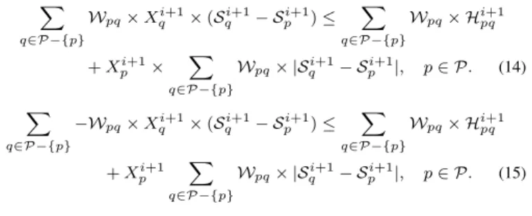
X q∈P−{p} Wpq× Hi+1pq + Xi+1p × X q∈P−{p} Wpq× |Sqi+1− Spi+1|, p ∈ P. (14) X q∈P−{p}
−Wpq× Xqi+1× (Sqi+1− Si+1p ) ≤
X q∈P−{p} Wpq× Hi+1pq + Xpi+1 X q∈P−{p} Wpq× |Sqi+1− Spi+1|, p ∈ P. (15)
The decision variable Hpqi+1 depends on Xqi+1 and Ei+1. We denote ε = E0 the initial maximum estimation error and it verifies Ei+1+ S
ep≤ ε, i ∈ N.
Therefore Hi+1pq respects the following constraints:
– If no sensor is redeployed towards point q, (Xi+1 q = 0):
0 ≤ Hi+1pq ≤ X i+1
q (16)
– If a sensor is redeployed towards point q, (Xqi+1= 1):
Ei+1+ Sep− (1 − X i+1 q ) × ε ≤ H i+1 pq ≤ E i+1 + Sep (17)
The corresponding denominator constraints is as follow:
X
q∈P−{p}
Wpq× Xqi+1> −Xpi+1, p ∈ P (18)
3) Mobility constraints: Previous mobility constraints are adapted to respect the limited search space as follows:
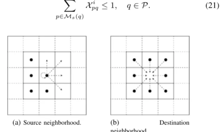
• Source constraints: At each iteration i, a source can only provide at maximum one sensor to one and only one of the cells in its Moore Extended Neighborhood denoted Me(p),
see Fig. 1.a.
Xpi =
X
q∈Me(p)
Xpqi , q ∈ P. (19)
• Destination constraints: At each iteration i, a destination q can receive at maximum one sensor from one and only one source in its Simple Moore Neighborhood Ms(q), see Fig.
1.b. Xqi+1= X p∈Ms(q) Xi pq, q ∈ P. (20)
• Collision constraints: Contrary to the optimal ILP model, the local redeployment regions of different sensors may overlap in LI2LP because the source and destination constraints are only satisfied in local neighborhoods. In order to avoid colli-sions, the LI2LP model ensures that a destination receives at maximum one sensor at each time point i. This is expressed by the constraints below:
X
p∈Ms(q)
Xi
pq≤ 1, q ∈ P. (21)
(a)Source neighborhood. (b) Destination neighborhood.
Fig. 1: Moore neighborhood and potential movement. 4) LI2LP model:At each iteration, the LI2LP model that provide the optimal local virtual movements between timestamps ti and
ti+1 is described as follows:
Objective : M inimize Ei+1
Pollution coverage constraints : (14), (15), (16), (17), (18) Sensors’ mobility constraints : (19), (20), (21)
5) LI2LP algorithm:The LI2LP model is repeatedly executed until no enhancement on the maximum estimation error is pos-sible. At each iteration, the output distribution Xi+1 is injected as the input distribution of the next iteration.
Algorithm 1: LI2LP model algorithm
Input: P deployment region, X0 sensors initial distribution, n number of deployed sensors
Output: Xf sensors final distribution
1 Evaluate initial maximum error E0 2 Ei+1, Xi+1← LI2LP model(Xi) 3 while Ei+1< Ei do
4 Ei← Ei+1
5 Xi← Xi+1
6 Ei+1, Xi+1← LI2LP model(Xi)
D. Heuristic algorithm
In this section, we present a redeployment heuristic based on local search and taboo list strategies. From the current distribu-tion, each sensors neighborhood is explored in order to find a potential destination that allows to enhance the global estimation quality.
1) Basic idea:The basic idea of this heuristic consists of enhanc-ing the global estimation quality by eliminatenhanc-ing points with high estimation errors. The algorithm tries to relocate neighboring sensors into these points. If no sensor can be directly redeployed to a point with high estimation error, the algorithm try to change the neighborhood sensors’ positions in order to reduce this high estimation error. Let Ei be the maximum estimation error in
the deployment region at a point p. In order to enhance the phenomenon coverage quality, a first sight solution is to directly redeploy a sensor towards point p. But, in some cases moving a :sensor in p’s vicinity may produce another point with higher estimation error. Thus, the alternative solution is to redeploy sensors into p’s vicinity. These redeployed sensors offer more precise reference values of p’s neighborhood allowing to enhance air quality estimation at point p using the interpolation function. 2) Heuristic algorithm:The first step of the heuristic algorithm is to assess all points p with estimation errors Epi > 0. According
to their error values, these points are grouped in a decreasing ordered list we call list of interest I. For each point p, we construct its candidates set C of neighboring sensors. The algo-rithm explores sequentially all potential movements of sensors s ∈ C. The first sensor’s movement that reduces the maximum error is validated and Ei and the interest list I are updated.
At the end of each iteration, if no movement is valid then the current considered point p is placed in a taboo list T . This list contains points to which no sensor can be redeployed. Once this list is full, all points in it are put back into I. In order to avoid oscillations effect of a sensor between two points, we use a movement history. At each iteration i if a sensor is redeployed, we save its previous position. When the same sensor is selected to be redeployed, once again, at iteration i + 1, we verify its destination. If the destination is saved in movement history as its previous position, then the movement is ignored, the sensor remains its current position.
This algorithm is executed iteratively until no point p ∈ I can be treated.
Algorithm 2: Heuristic algorithm
1 Construct interest list I in error decreasing order 2 while I 6⊆ T do
3 Select first point p in I − T
4 Construct C the sensors candidates set of p in distance increasing order
5 for each sensor s in C do
6 Simulate sensor s movement to p 7 Evaluate Ei+1
8 if Ei> Ei+1then
9 Add s’s movement to valid movements list and movements history
10 Update I
11 if no valid movement then
12 Add p to T
V. SIMULATION RESULTS
A. Data set
We perform our evaluation using real pollution maps of nitrogen dioxide (N O2) concentrations on La Part-Dieu district, of Lyon
City in France. The data set is provided by Air-Rhone-Alpes an observatory for air pollution monitoring using an atmospheric dispersion simulator called SIRANE [14]. These maps are con-sidered as reference maps (the simulation errors are assumed to be negligible). We considered for our tests a deployment region of 1 km2, that we discretized using a resolution of 50 meters. B. Proof of concept
To validate our proposed strategies, we first run the redeployment models on pollution reference map shown in Fig.2.c with an initial deployment of 150 sensors. The obtained error maps are shown on Fig.2.d, Fig.2.e and Fig.2.f.
(a)Deployment region real map. (b)N O2concentrations (10 meter res-olution).
(c)N O2concentrations (50 meter res-olution).
(d)Initial random deployment.
(e)LI2LP Model. (f)Heuristic Model.
Fig. 2: Initial and final (after redeployment) estimation errors. We notice that points with high estimation errors (darker cells) are considerably less present in resulting maps than in the initial map. The error maps show that the LI2LP model offers better results since cells with significant errors (dark cells)
are considerably reduced compared to the heuristic model. We also observe that more nodes are involved in the redeployment process. The high mobility in LI2LP model comes with an additional cost in time and energy.
C. Performance evaluation
In this section we analyze redeployment models’ performance according to maximum estimation error and execution time. The following presented results are obtained using over 200 different initial map instances per configuration with a confidence level of 98%.
1) maximum error:We present in Fig.3 the average maximum initial error as well as the average maximum estimations errors resulting from our redeployment strategies according to deployed sensors’ number. The proposed redeployment strategies allow to significantly reduce the initial maximum errors down to 60% in worst cases. Deploying more sensors decreases the maximum estimation error, because it allows to have more reference values for the interpolation-based estimation and thus more precise estimated values. The ILP model presents, as expected, the best results while the maximum estimation error given by LI2LP model is relatively more important. The difference between both models decreases from 36% in sparse deployments down to 20% in deployments with a higher number of sensors. The curves of these two models come closer when the number of sensors increase which is due to the convergence of search spaces of the two models in dense configurations. The heuristic model offers less significant enhancement than both ILP and LI2LP, it allows to reduce the maximum estimation error to 30% of its initial value in average. With more deployed sensors, the space search becomes more and more limited. Therefore, the global redeployment schemes for different initial deployments are almost similar and the error margins decrease with the increase of deployed sensors.
Fig. 3: Average maximum estimation error.
2) Execution time:As we mentioned before, the major draw-back of the optimal ILP model is the important computation time which isn’t suitable for timely monitoring of the studied phenomena. We analyze both LI2LP and the heuristic execution time according to the number of deployed sensors as depicted in Fig. 4. From the first sight, we note that both LI2LP and the heuristic have an execution time of few minutes at maximum, instead of few hours for the optimal ILP model (see Table (II)). Indeed, the execution time enhancement factor compared the ILP model goes from 120 times in dense deployments up to 700 times in sparse deployments. Moreover, we notice that, as when using
the ILP model, the execution time decreases with the increase of the number of deployed sensors. This is mainly due to the reduction of the search space with the increase of the number of deployed sensors. Finally, we notice the LI2LP model is, in average, 3 times slower than the heuristic (see Fig. 4.).
Fig. 4: Models’ execution time. D. Comparison with state of art strategies
To evaluate the quality of our models, we compare them to a state of art redeployment strategy called SMART [17]. SMART is a grid-based optimal redeployment strategy that offers a high level uniform coverage with fast convergence. Fig.5 depicts the average maximum estimation error of 200 simulations for each sensors number. The obtained results showed that our models are at least 50% better than those obtained using SMART. Moreover, this ratio increases with the number of sensors. For instance, in deployments with over 300 sensors, the maximum error given by our models is under 5µg/m3, while it is around 14µg/m3
for SMART model (i.e. our results are 3 times better).
Fig. 5: Performance comparison with SMART strategy. VI.CONCLUSION
In this work, we focused on the use of mobile WSN for online continuous air pollution monitoring. First, we gave a redeploy-ment problem formulation considering air pollution dynamics and dispersion models in order to reduce air quality estimation errors. Then, we proposed an exact optimal resolution model based on integer linear programming (ILP). After that, we presented two approximate resolution methods based on local iterative ILP model and local search technique, respectively. We evaluated our models’ performance in terms of the maximum estimation error and execution time using a dataset of Lyon City in France. We highlighted the performances, advantages and
drawbacks of each strategy. Finally, we compared our obtained results to a state of art redeployment strategy.
ACKNOWLEDGMENT
This work has been partly funded by the SPIE ICS - INSA Lyon Chair on Internet or Things. It has also been partially supported by the Labex IMU (ANR-10-LABX-0088) of Universit´e de Lyon, within the program ”Investissements d’Avenir” (ANR-11-IDEX-0007) operated by the French National Research Agency (ANR).
REFERENCES
[1] World Health Organisation. WHO: Ambient (outdoor) air quality and health, publi´e: 2016-09. Acc`es: 2017-05. http://www.who.int/mediacentre/factsheets/fs313/en/.
[2] Mark Z Jacobson and Yoram J Kaufman. Wind reduction by aerosol particles. Geophysical Research Letters, 33(24), 2006.
[3] Ali Marjovi, Adrian Arfire, and Alcherio Martinoli. High resolution air pollution maps in urban environments using mobile sensor networks. In IEEE DCOSS2015, pp 11–20, IEEE.
[4] Ahmed Boubrima, Walid Bechkit, and Herv´e Rivano. Error-bounded air quality mapping using wireless sensor networks. In IEEE LCN 2016, pp 380–388, IEEE.
[5] Ahmed Boubrima, Walid Bechkit, and Herve Rivano. Optimal wsn deployment models for air pollution monitoring. IEEE TWC 2017. [6] Mustapha Reda Senouci, Abdelhamid Mellouk, Khalid Asnoune, and
Fethi Yazid Bouhidel. Movement-assisted sensor deployment algorithms: A survey and taxonomy. In IEEE CST 2015, pp 2493–2510, IEEE. . [7] Krishnendu Chakrabarty, S Sitharama Iyengar, Hairong Qi, and Eungchun
Cho. Grid coverage for surveillance and target location in distributed sensor networks. In IEEE TC 2002, pp 1448–1453, IEEE.
[8] M Emre Keskin, ˙I Kuban Altınel, Necati Aras, and Cem Ersoy. Wireless sensor network lifetime maximization by optimal sensor deployment, activity scheduling, data routing and sink mobility. Ad Hoc Networks, 17:18–36, 2014.
[9] Maher Rebai, Hichem Snoussi, Faicel Hnaien, Lyes Khoukhi, et al. Sensor deployment optimization methods to achieve both coverage and connec-tivity in wireless sensor networks. Computers & Operations Research, 59:11–21, 2015.
[10] Dina S Deif and Yasser Gadallah. Classification of wireless sensor networks deployment techniques. In IEEE CST 2014, pp 834–855, IEEE. [11] Guiling Wang, Guohong Cao, and Thomas F La Porta. Movement-assisted
sensor deployment. IEEE TMC 2006, pp 640–652, IEEE.
[12] Xueqing Wang, Yongtian Yang, and Yibing Song. Redundant movement-assisted sensor deployment based on virtual rhomb grid in wireless sensor networks. In Mechatronics and Automation, Proceedings of the 2006 IEEE International Conference on, pages 775–779. IEEE, 2006.
[13] Andrew Howard, Maja J Matari´c, and Gaurav S Sukhatme. Mobile sensor network deployment using potential fields: A distributed, scalable solution to the area coverage problem. In Distributed Autonomous Robotic Systems 5, pages 299–308. Springer, 2002.
[14] Lionel Soulhac, Pietro Salizzoni, Patrick Mejean, D Didier, and I Rios. The model sirane for atmospheric urban pollutant dispersion; part ii, validation of the model on a real case study. Atmospheric environment, 49:320–337, 2012.
[15] Despina Deligiorgi and Kostas Philippopoulos. Spatial interpolation methodologies in urban air pollution modeling: application for the greater area of metropolitan Athens, Greece. INTECH Open Access Publisher, 2011.
[16] Eric W Weisstein. Moore neighborhood. From MathWorld–A Wolfram Web Resource. http://mathworld. wolfram. com/MooreNeighborhood. html, 2005.
[17] Jie Wu and Shuhui Yang. Optimal movement-assisted sensor deployment and its extensions in wireless sensor networks. Simulation Modelling Practice and Theory, 15(4):383–399, 2007.