HAL Id: hal-01346316
https://hal.archives-ouvertes.fr/hal-01346316
Submitted on 20 Jul 2016
HAL is a multi-disciplinary open access
archive for the deposit and dissemination of
sci-entific research documents, whether they are
pub-lished or not. The documents may come from
teaching and research institutions in France or
abroad, or from public or private research centers.
L’archive ouverte pluridisciplinaire HAL, est
destinée au dépôt et à la diffusion de documents
scientifiques de niveau recherche, publiés ou non,
émanant des établissements d’enseignement et de
recherche français ou étrangers, des laboratoires
publics ou privés.
High-precision helium isotope measurements in air
J Mabry, T.F. Lan, P.G. Burnard, Bernard Marty
To cite this version:
J Mabry, T.F. Lan, P.G. Burnard, Bernard Marty. High-precision helium isotope measurements in air.
Journal of Analytical Atomic Spectrometry, Royal Society of Chemistry, 2013, �10.1039/c3ja50155h�.
�hal-01346316�
Journal Name
Cite this: DOI: 10.1039/c0xx00000x
www.rsc.org/xxxxxx
Dynamic Article Links
►
ARTICLE TYPE
High-precision helium isotope measurements in air
Jennifer Mabry,*
aTefang Lan,
aPete Burnard
aand Bernard Marty
aReceived (in XXX, XXX) Xth XXXXXXXXX 20XX, Accepted Xth XXXXXXXXX 20XX
DOI: 10.1039/b000000x
Helium has two natural isotopes which have contrasted, and variable sources and sinks in the atmosphere
5
(3He/4He
air = 1.382 ± 0.005 x 10⁻⁶). Variations in atmospheric helium isotopic composition may exist
below typical measurement precision thresholds (0.2 to 0.5%, 2σ). In order to investigate this possibility, it is necessary to be able to consistently measure helium isotopes in air with high precision (below 0.2% 2σ). We have created an air purification and measurement system that improves the helium isotope measurement precision. By purifying a large quantity of air at the start of a measurement cycle we can
10
make rapid standard-bracketed measurements. Controlling the amount of helium in each measured aliquot minimizes pressure effects. With this method we improve the standard errors by 2x over measuring the same amount of gas in a single step. Individual measurements have standard errors of 0.2 to 0.3% (2σ), with three repeat samples needed to reach 0.1% or better errors. The long-term reproducibility of our calibration sample is 0.033% (2σ).
15
Introduction
The atmospheric content of helium (5.24 ppm vol.1) is much
lower than would be predicted from degassing of the mantle and crust because helium escapes from the atmosphere through thermal and non-thermal processes2. Therefore, the atmospheric 20
abundance of its two natural isotopes, 3He and 4He, results from a
balance of outgassing of the solid earth, input from precipitation of solar wind at the poles, and loss into space, with a residence time on the order of 106 years3. The isotopic composition of the
atmosphere (3He/4He = 1.382 ± 0.005 x 10⁻⁶)4 is distinctly
25
different from crustal helium (3He/4He ~10-8) which is dominated
by radiogenic 4He produced during the alpha decays of crustal U
and Th. Several authors5–7 have proposed that the amount of
excess crustal helium entering the atmosphere due to modern fossil fuel extraction may be enough to upset the balance of the
30
helium composition in the atmosphere on a timescale short enough to detect with modern measurement techniques.
Several groups have searched for evidence of temporal6–12
variations in the helium isotopic composition of the atmosphere, however results thus far have not been definitive. Groups6,7,11 35
measuring pre-industrial samples report elevated 3He/4He relative
to modern air by as much as 4%, but the errors associated with these measurements are typically quite large, up to 50%. Groups searching for temporal variations on a shorter, decadal scale have found a range of results from no change at the 0.2% (2σ) level10, 40
to a decrease of the atmospheric 3He/4He of (0.023 ±
0.008)%/year12 up to (0.094± 0.156)%/year9. In order to resolve
these discrepancies will require further improvement in the
precision of 3He/4He measurements from air samples.
Obtaining such a high level of precision (below 0.2%) for
45
helium measurements presents several analytical challenges. The low abundance of helium in the atmosphere means that large quantities of air must be well-purified to obtain a reasonable helium signal and that static mass spectrometry must be used. High-sensitivity noble gas ion sources are notorious for being
50
pressure sensitive, which means it is imperative to closely match the amounts of gas measured in each sample or standard aliquot. There are six orders of magnitude difference in abundance of the two isotopes of helium, making simultaneous detection challenging. Finally, 3He has several isobars, which must either 55
be resolved or corrected for.
In this paper, we detail the system we have developed in order to mitigate these challenges. It features a unique standard-sample bracketing system that will mimic as closely as possible the rapid switching between standard and sample which is possible with
60
dynamic mass spectrometry. Our system allows the purification and preparation of enough sample gas for multiple analyses of the same sample, thus gaining some of the benefits of the dynamic system. Additionally, the amount of helium in each sample aliquot is matched to the amount in an aliquot of the standard to
65
minimize pressure effects. Data acquired by this method are compared to the more standard measurement technique of measuring all of the purified sample in a single aliquot for statistical comparison.
Journal Name
Cite this: DOI: 10.1039/c0xx00000x
www.rsc.org/xxxxxx
Dynamic Article Links
►
ARTICLE TYPE
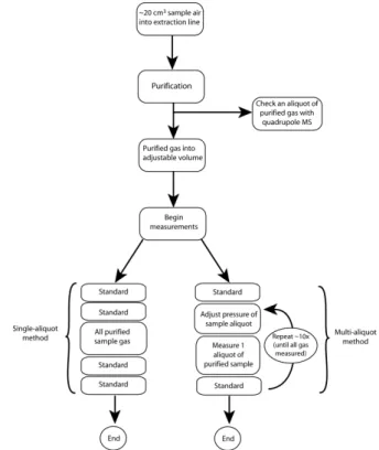
This journal is © The Royal Society of Chemistry [year] [journal], [year], [vol], 00–00 | 2 Fig. 1 Schematic of the sample purification and inlet system.
Method
Sample Gas Purification
We purify a relatively large amount of air sample (~15-20 cm3) 5
all at once before any measurements are made. The air is first exposed to activated charcoal held at 77K (liquid nitrogen temperature) to trap the majority of the unwanted gases including the heavier non-reactive gases such as argon. Then the remaining gas is sequentially exposed to two hot (~400C) titanium getters
10
which chemically trap reactive gases and to an additional activated charcoal finger (Fig. 1A). Each step lasts ten minutes. In order to monitor the consistency of the purification from sample to sample, we separate a small amount of the purified gas and analyze it with a quadrupole mass spectrometer (MKS
15
Microvision 2™, Fig. 1C). After purification, each sample consists of > 98% neon and helium isotopes and < 2% impurities (such as H2, N2 and CO2). Regular repetitions show no significant
variations.
The purified sample is then held in an adjustable volume (Fig.
20
1D) with a pipette (Fig. 1E) which is used to take multiple aliquots and perform standard-sample bracketing. Repeated measurements draw on the same reservoir of purified sample, which is important, as typically using a “standard bracketing” method with static mass spectrometry actually means using a
25
newly purified sample for each measurement13.
Running Standard and Sample Air
The standard we used for our standard bracketing measurements
is a bottle of purified air obtained from the Bretagne region of
30
France, just on the shore of the Atlantic. A 2.3L volume of air was collected in a steel tank and passed through silica gel to remove some of the water. This gas was later purified in the lab. The air was sequentially exposed to two titanium getters (~800C) for approximately 125 hours and then to cold (77K) activated
35
charcoal for 2.5 hours. Finally the gas was expanded into a 10L bottle with a 0.1 cm3 pipette for use. Twice, we expanded this
bottle to a portion of our extraction line for approximately 15 hours in order to expose it to activated charcoal and remove further traces of argon and other impurities.
40
For the sample measurements described in this paper we use air that was collected in a 2.3L tank from a park on a bluff near the CRPG Institute: Parc de Brabois, Villers-lès-Nancy, France (48.661 N , 6.149 E). This location is 85 km from the closest nuclear power plant; the closest industrial plant is a steel factory
45
about 7 km away. This bottle is connected to an ~7 cm3 pipette
volume. From this tank we draw approximately 20 cm3 (3
pipettes to start, increasing as the tank becomes depleted) of air for each measurement. This volume is sufficient to take multiple measurement aliquots from each sample after purification.
50
We used an air standard, rather than an artificially mixed standard which could have a higher 3He content (and thus lower
error associated with our calibrations), because we wanted the standard and sample to be as close as possible in composition to eliminate biases in the mass spectrometer. However, despite
55
precautions, the standard gas is fractionated relative to Brabois air, being depleted in 3He by 3.6%. This fractionation was
discovered early on in the life of the standard and has remained stable over time. Thus we believe that it occurred during the
preparation of the standard.
We have considered several possible sources of this fractionation and found them all to be improbable. The long times during purification make it unlikely that a light gas such as helium would be fractionated by thermal diffusion. We also
5
considered thermophoresis, which can cause steady state concentration gradients under some conditions, but this effect should be negligibly small for helium atoms at atmospheric or lower pressure14. Finally, the possibility that large enough
quantities of helium were adsorbed on the silica gel at room
10
temperature to cause such a level of fractionation is not plausible15. Thus further experiments would be needed to
determine the cause of the fractionation, which is beyond the scope of this work.
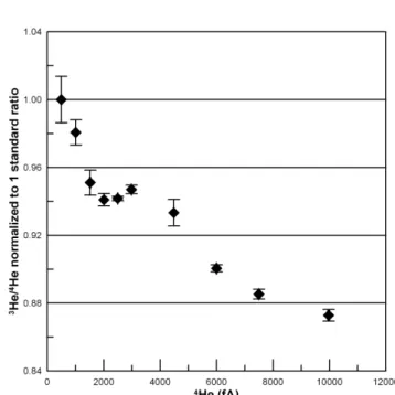
Pressure Effect
15
It is essential to control the amount of gas let into the mass spectrometer with each measurement, because the ion source (Nier-type) is extremely sensitive to pressure16. For example, in
measuring multiples of our standard, we found the measured
3He/4He ratio changes nonlinearly by about 13% for a 20-fold 20
increase in the 4He amount (Fig. 2). Mitigating this effect was
one of the major considerations when designing this new method, and we approach the problem in two steps.
First, the volume where the purified sample gas is held is adjustable, consisting of a bellows connected to a stepper motor
25
which is computer controlled. This serves two purposes: (1) to allow us to match the amount of gas in a sample aliquot with the size of an aliquot of our standard (since different samples can have different amounts) and (2) to compensate for the depletion of the reservoir as aliquots are pulled out and the pressure
30
decreases. Carefully matching the size of each sample aliquot to the standard and previous sample aliquots bypasses the need for a pressure correction in the data. In practice we found that keeping the 4He amount of the sample within 2% of the standard amount
was close enough to eliminate the pressure effect. This level was
35
chosen because there are no correlations with amount seen at this
level (Fig. 3). At the 10% variation, there is a clear correlation between the amount and the ratio, but this disappears at the 2% level. 40 Fig. 2
Effect of the pressure in the mass spectrometer on the measured 3 He/4He ratio. The ratio decreases nonlinearly by about 13% for a 20‐fold increase in 4 He amount.
Second, we expose both the sample gas and standard gas to a
45
cryogenic trap (Oxford ICE, Fig. 1G) to remove the neon before admittance to the mass spectrometer. The trap is set to 35K (uncalibrated temperature, set point determined experimentally where most neon is trapped without trapping helium) and is stable to ± 0.01K. This keeps the pressure in the mass spectrometer as
50
low and as consistent as possible.
Fig.3 Measured 3He/4He ratio for different varying amounts of 4He relative to the internal standard: a) all measurements, some which have 40% different 4He amount from the standard; b) filtering out points more than 5% away from the standard amount; and c) filtering out points more than 2%
55
4 | Journal Name, [year], [vol], 00–00 This journal is © The Royal Society of Chemistry [year]
Fig. 4 Single measurements of 4He with an activated charcoal finger on the mass spectrometer volume: (a) adding roughly 2 cm of liquid N2 near end of
the measurement, (b) without any liquid N2, and (c) after replacing the charcoal finger with a cryogenic trap.
5
Mass Spectrometer
Measurements are made on a new Thermo Helix Split Flight Tube (SFT) multi-collector noble gas mass spectrometer, which was installed in February 2012. This machine is designed for helium isotope measurements with a split flight tube which
10
physically separates the 3He and 4He beams. The two paths terminate in an electron multiplier and Faraday cup to allow for simultaneous detection of 3He and 4He. The mass resolution of
the multiplier is ~700 which is sufficient to resolve 3He isobars
(HD and 3H), and the resolution of the Faraday cup is 425. An 15
electrostatic filter before the multiplier helps to further improve isotope separation and block out stray ions. The helium sensitivity is 2.35×10⁻⁴ A/torr at 400 µA trap current. We
typically operate at 350 µA trap current and 4500V acceleration voltage.
20
An SAES getter installed on the mass spectrometer volume keeps hydrogen levels low which reduces the amount of HD interference at mass 3. Previously, a charcoal finger was used to keep the background of argon and other heavier isotopes low during a static measurement. However, we found that for these
25
measurements, it was not stable enough and the small pressure changes resulting from modest changes to the liquid nitrogen level were enough to disrupt the measurement (Fig. 4). For example, the addition of approximately 2 cm of liquid N2 could
change the sensitivity of the 4He measured by 2% (Fig. 4a). 30
Filling the liquid N2 only before an analysis (and not during)
sometimes worked, but could have unpredictable effects depending on the length of the analysis and the temperature in the room which would change how much evaporation occurred over the course of the measurement. Abandoning liquid N2 altogether 35
(Fig. 4b) made for very unstable measurements. These problems disappeared with the replacement of the charcoal finger by the cryogenic trap (Fig. 4c). This trap is set to 25K (uncalibrated temperature, set point determined experimentally at lowest temperature not trapping helium) and is stable to ± 0.05K.
40
Measurements and Results
In order to evaluate whether the changes to our extraction line and measurement method led to a real improvement in the statistics of the measured data, we performed two different sets of
45
measurements over the course of three months. All of these measurements were made using the Brabois (local air) sample gas tank as described above.
50
Fig. 5 Flow diagram of the procedure for the single‐aliquot and multi‐
aliquot methods.
We made a set of measurements employing the multiple standard bracketed technique described above, making multiple measurements of each sample. And to compare with this, we also
55
amount of sample gas but then letting all of the gas into the mass spectrometer for a single measurement of each sample, also bracketed by measurements of the standard. These will be referred to as the multi-aliquot and single-aliquot methods respectively. The initial procedure such as gas purification is
5
identical for both methods, only the measurement procedure differs (Fig. 5). The total amount of gas measured by each method is approximately the same, however the total time of the measurement is much less for the single-aliquot method: ~15 minutes for the single-aliquot vs ~150 minutes over all
10
measurements for the multi-aliquot method.
Multi-Aliquot Measurements
To perform the multi-aliquot measurements, approximately 20 cm3 of air is purified and passed through the extraction line to the
bellows volume as described above. A small aliquot of this gas is
15
quickly measured in the mass spectrometer to determine the pressure of He in the bellows volume and then the bellows position is adjusted such that the amount of 4He in one aliquot is
within 2% of the amount in one pipette of the standard. Once this is reached, the measurement proceeds with multiple sample
20
aliquots being drawn out from the bellows volume for separate measurements, each one bracketed by standard measurements (Fig. 5). The total time for sample preparation and measurement is around 9 hours.
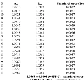
Table 1 Multi-aliquot measurement data. Shown are the total number of
25
measurements (N), the average measured 4He relative to the standard
(Am), the average 3He/4He relative to the standard (Rm), and the standard
error (2σ). N Am Rm Standard error (2σ) 11 0.9910 1.0387 0.0022 11 1.0116 1.0359 0.0031 10 0.9923 1.0356 0.0017 8 1.0041 1.0354 0.0033 8 0.9810 1.0354 0.0032 11 1.0045 1.0372 0.0029 11 1.0138 1.0364 0.0029 11 1.0043 1.0368 0.0026 9 1.0079 1.0346 0.0021 11 0.9991 1.0346 0.0012 6 1.0071 1.0352 0.0043 11 0.9882 1.0361 0.0022 11 0.9921 1.0377 0.0020 11 0.9914 1.0361 0.0037 11 0.9883 1.0378 0.0022 9 0.9960 1.0367 0.0019 11 0.9991 1.0379 0.0027 11 0.9955 1.0355 0.0033 11 0.9862 1.0363 0.0030 1.0363 ± 0.0005 (0.051%) – standard error ± 0.0023 (0.22%) – standard deviation 30
Table 1 summarizes the measurements made by the multi-aliquot method. The quantity Am in Table 1 represents how closely the amount of helium in the sample measurements is matched to the standard. First, the aliquot amount, Aa, is calculated, as the measured 4He of the sample aliquot, divided by 35
the average of the amounts in the standards measured immediately before and after the sample aliquot:
2 .
Then for each sample, the average of all of the individual Aa are made to give the final for the sample: ∑ ⁄ , where N is the number of standard-bracketed aliquots measured from
40
that sample. Typically, it is possible to measure 11 aliquots from one sample, however if the value of Aa was greater than 1.02 or less than 0.98 (i.e. if the amount of 4He in a sample aliquot
differed than the standard by more than ±2%), then that measurement was thrown out.
45
The ratios, Rm (Table 1) are calculated the same way as the amounts. First, the aliquot ratio, Ra, is calculated, as the measured
3He/4He of the sample aliquot, divided by the average of the
measured ratios of the standards measured immediately before and after the sample aliquot:
50
2 .
Then for each sample, the average of all of the individual Ra are made to give the final for the sample: ∑ ⁄ . The standard errors (2σ) are between 0.2% and 0.3% for one sample. This error is dominated by the scatter in the 3He measurement.
For the 19 measurements shown, the average value is 1.0363 with
55
a standard error (2σ) well below 0.1% at 0.0005 (0.051%).
Single-aliquot measurements
To perform single-aliquot measurements, the procedure is identical to that of the multi-aliquot measurements for gas purification (Fig. 5). However, for the actual measurement, all of
60
the sample gas is let into the mass spectrometer and measured at once. Two standards are measured before the sample gas, and two more after. The total time for sample preparation, standard and sample measurement is around 3 hours.
Table 2 Single-aliquot measurement data. The average measured 4He 65
relative to the standard (As), the average 3He/4He relative to the standard
(Rs), and the standard error (2σ) are shown.
As Rs Standard error (2σ) 13.51 0.9238 0.0034 13.38 0.9281 0.0044 13.54 0.9273 0.0033 13.59 0.9272 0.0023 13.64 0.9264 0.0029 13.45 0.9281 0.0036 13.51 0.9288 0.0067 13.56 0.9272 0.0037 13.56 0.9269 0.0023 13.53 0.9260 0.0035 13.61 0.9252 0.0050 13.62 0.9246 0.0025 13.64 0.9281 0.0026 13.53 0.9307 0.0030 13.56 0.9243 0.0030 13.52 0.9293 0.0034 13.43 0.9236 0.0039 0.9268 ± 0.0010 (0.105%) – standard error ± 0.0040 (0.42%)– standard deviation
6 | Journal Name, [year], [vol], 00–00 This journal is © The Royal Society of Chemistry [year]
As with the multi-aliquot measurements, we show (Table 2) the amount of gas in the single sample aliquot relative to the standard (As), which is the amount of 4He in the sample aliquot divided by the average of the two standards measured before and
5
the two standards measured after:
∑ ⁄4.
In contrast to the multi-aliquot method, we are not trying to match the sample size to the standard, but simply to match the amount of helium between one sample and the next. We rejected any data that varied by more than ±2% from the mean of all the
10
As values.
The ratio Rs is also relative to the average ratios measured from the standards measured with the sample:
∑ ⁄4.
The errors given for each ratio are the calculated errors based on the measurement error of the five (four standards, one sample)
15
individual measurements and are typically 0.3% to 0.4% for each single measurement. The mean for these 17 measurements is 0.9268 with standard error is 0.001 (0.1%, 2σ). Note that this ratio differs from the multi-aliquot ratio (by ~11%). This is a consequence of the pressure effect discussed above; although
20
both are normalized to the same internal standard, the single-aliquot measurements have about 13.5 times more gas than the multi-aliquot measurements.
Discussion
For purposes of comparing these two measurement methods, we
25
have normalized these two data sets to their respective mean values and show them together in Fig. 6. Each point represents approximately the same total amount of sample gas measured. The multi-aliquot method has noticeably less amount of scatter and the standard deviation is half that of the single-aliquot data.
30
Fig. 6 Normalized measured ratios for the single‐aliquot (purple circles)
and multi‐aliquot (black diamonds) method, shown in the order in which
they were measured. The inner shaded region represents one standard deviation for the multi‐aliquot measurements, while the out shaded
35
region is one
standard deviation for the single‐aliquot measurements.
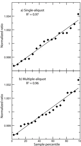
Fig. 7 Normal probability plot for (a) single‐aliquot and (b) multi‐aliquot
ratio measurements.
40
To determine whether or not the difference between these two methods is statistically significant, we make a one-tailed F-test. First, for the test to be valid the data sets should be normally distributed, so we make a normal probability plot for each data set (Fig. 7) and check that the result is linear. We use a one-sided
45
test because we developed the multi-aliquot method specifically to improve upon the single-aliquot method. The details of this calculation are shown in Table 3 and indicate that the lower variance of the multi-aliquot method compared to the single-aliquot method is statistically significant at a 95% confidence
50
Table 3 One-tailed F-test calculation comparing the standard deviations
of the multi-aliquot (Sm) and single-aliquot (Ss) measurements. The
calculation indicates that the difference between them is significant. Formulate null and alternative
hypotheses
H0 Sm2 = Ss2
H1 Sm2 < Ss2
Calculate F F = Ss2/ Sm2 = (0.00200)2/(0.00111)2
= 3.2465 Critical F value for α = 0.05 Fcrit = 2.2496
Is F > Fcrit? 3.2465 > 2.2496
In a direct comparison, for the same total amount of gas
5
measured, but different total measurement times, the multi-aliquot method has errors on a single sample of about 60% of the single-aliquot method and a long term reproducibility that is about twice as good. Although it seems obvious that increasing the measurement time will improve the statistics, this is not
10
always the case. A significant increase in measurement time, such as in this case, increases the probability that external factors (drift in electronics, gain of detectors, temperature, day/night variations) may affect the measurement and thus hinder an improvement in statistics.
15
Next, there is the question of whether the improvement is worth the extra measuring time. This depends on several factors such as the time available for measurements, the precision needed, and the number of samples available. Based on these data, it takes only on average 3 separate sample measurements by
20
the multi-aliquot method to reach a standard error of 0.1% (2σ) for a total laboratory time around 30 hours. In contrast, the single-aliquot method approached a plateau at an average standard error of 0.11% (2σ) after 11 separate samples measured (total laboratory time ~33 hours). Thus, if reaching 0.1%
25
precision is important, the multi-aliquot method is the better choice, especially if one is limited in the number of samples one can acquire.
Finally, we have made measurements using the multi-aliquot method over an extended time period beyond this comparison
30
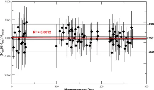
study in order to assess the long-term reproducibility. The measurements made over a period of about 270 days were very
stable (Fig. 8), with no trend detected; a linear fit gives an R2 =
0.0012. This time period includes the replacement of the multiplier around day 200 (necessitating opening the mass
35
spectrometer to atmosphere).
The 2σ standard error over this entire period is 0.033%. The earliest measurements (first 30 days) have a higher amount of scatter (SD = 0.41% 2σ) compared to later measurements (SD = 0.27% 2σ). We attribute this to the fact that the first
40
measurements were made soon after the installation of the new mass spectrometer and some details were still being finalized such as climate control of the laboratory.
Conclusions
We have constructed an extraction line to purify relatively large
45
quantities of atmospheric helium and monitor the consistency of the purification process with a quadrupole mass spectrometer. An adjustable volume is used to control the quantity of this helium to be let into the mass spectrometer and thus mitigate pressure effects in the source. A cryogenic trap on the line removes the
50
neon from the sample gas for further control of the pressure in the mass spectrometer. The addition of a second cryogenic trap on the mass spectrometer volume maintains low and stable background levels which are essential for high precision helium isotope measurements.
55
We compared our modified multi-aliquot measurement method to the more ‘traditional’ single-aliquot method. In both cases we monitor and control the amount of gas let in for a measurement. We found a 2x improvement in the error when using the multi-aliquot measurement technique over the single-multi-aliquot method.
60
With the multi-aliquot measurement technique, we can measure with a long-term reproducibility over several months of 0.033% (2σ). Single measurements have standard errors of 0.2 to 0.3% (2σ), but only three replicate samples are needed to reach 0.1% or better errors. This is a level sufficient to probe further into the
65
question of temporal helium isotopic variations.
Fig. 8 All (83) multi‐aliquot measurements made over 270 days. The red line is a linear fit of the data and shows no significant trend over time. The grey
shaded area shows 2 standard errors (SE) and the thick black lines show 2 standard deviations (SD).
Journal Name
Cite this: DOI: 10.1039/c0xx00000x
www.rsc.org/xxxxxx
Dynamic Article Links
►
ARTICLE TYPE
This journal is © The Royal Society of Chemistry [year] [journal], [year], [vol], 00–00 | 8
Acknowledgments
This experiment is funded by grant VIHA2 from the Agence Nationale de la Recherche (ANR), and by the European Research Council under the European Community’s Seventh Framework Programme (FP7/2007-2013 grant agreement no. 267255).
5
Notes and references
a CRPG-CNRS, 15 rue Notre Dame des Pauvres, Vandoeuvre-les-Nancy,
France. E-mail:[email protected]
1. E. Gluckauf, Proceedings of the Royal Society A: Mathematical,
10
Physical and Engineering Sciences, 1946, 185, 98–119. 2. G. Kockarts and M. Nicolet, Ann. Geophys., 1962, 18, 269–290. 3. T. Torgersen, Chemical Geology: Isotope Geoscience section, 1989,
79, 1–14.
4. Y. Sano, B. Marty, and P. Burnard, in The Noble Gases as
15
Geochemical Tracers, ed. P. Burnard, Springer, 2013, pp. 17–31. 5. B. M. Oliver, J. G. Bradley, and H. Farrar IV, Geochimica et
Cosmochimica Acta, 1984, 48, 1759–1767.
6. A.-C. Pierson-Wickmann, B. Marty, and A. Ploquin, Earth and Planetary Science Letters, 2001, 194, 165–175.
20
7. Y. Sano, Y. Furukawa, and N. Takahata, Geochimica et Cosmochimica Acta, 2010, 74, 4893–4901.
8. Y. Sano, H. Wakita, Y. Makide, and T. Tominaga, Geophysical Research Letters, 1989, 16, 1371–1374.
9. Y. Sano, Journal of Science of the Hiroshima University, 1998, 11,
25
113–118.
10. J. Lupton and L. Evans, Geophys. Res. Lett., 2004, 31, 4.
11. J.-I. Matsuda, T. Matsumoto, and A. Suzuki, Geochemical Journal, 2010, 44, e5–e9.
12. M. S. Brennwald, N. Vogel, S. Figura, M. K. Vollmer, R.
30
Langenfelds, L. Paul Steele, C. Maden, and R. Kipfer, Earth and Planetary Science Letters, 2013, 366, 27–37.
13. Y. Sano, T. Tokutake, and N. Takahata, Analytical sciences: The international journal of the Japan Society for Analytical Chemistry, 2008, 24, 521–5.
35
14. R. Piazza, Soft Matter, 2008, 4, 1740.
15. D. S. Tomar, M. Singla, and S. Gumma, Microporous and Mesoporous Materials, 2011, 142, 116–121.
16. P. G. Burnard and K. A. Farley, Geochemistry Geophysics
Geosystems, 2000, 1, 1022.