HAL Id: hal-03218055
https://hal.archives-ouvertes.fr/hal-03218055
Submitted on 6 May 2021
HAL is a multi-disciplinary open access
archive for the deposit and dissemination of
sci-entific research documents, whether they are
pub-lished or not. The documents may come from
teaching and research institutions in France or
abroad, or from public or private research centers.
L’archive ouverte pluridisciplinaire HAL, est
destinée au dépôt et à la diffusion de documents
scientifiques de niveau recherche, publiés ou non,
émanant des établissements d’enseignement et de
recherche français ou étrangers, des laboratoires
publics ou privés.
Distributed under a Creative Commons Attribution - NonCommercial - NoDerivatives| 4.0
International License
Two methods for estimating limits to large-scale wind
power generation
Lee Miller, Nathaniel Brunsell, David Mechem, Fabian Gans, Andrew
Monaghan, Robert Vautard, David Keith, Axel Kleidon
To cite this version:
Lee Miller, Nathaniel Brunsell, David Mechem, Fabian Gans, Andrew Monaghan, et al.. Two methods
for estimating limits to large-scale wind power generation. Proceedings of the National Academy of
Sciences of the United States of America , National Academy of Sciences, 2015, 112 (36),
pp.11169-11174. �10.1073/pnas.1408251112�. �hal-03218055�
Two methods for estimating limits to large-scale wind
power generation
Lee M. Millera,1, Nathaniel A. Brunsellb, David B. Mechemb, Fabian Gansa, Andrew J. Monaghanc, Robert Vautardd, David W. Keithe, and Axel Kleidona
aMax Planck Institute for Biogeochemistry, 07701 Jena, Germany;bUniversity of Kansas, Lawrence, KS 66045;cNational Center for Atmospheric Research,
Boulder, CO 80305;dLaboratoire des Sciences du Climat et de l’Environnement, Institut Pierre-Simon Laplace, Laboratoire Commissariat à l’Énergie
Atomique, CNRS, Université de Versailles Saint-Quentin-en-Yvelines, Gif/Yvette Cedex, 78000 Versailles, France; andeHarvard University, Cambridge, MA
02138
Edited* by Christopher J. R. Garrett, University of Victoria, Victoria, BC, Canada, and approved June 25, 2015 (received for review May 6, 2014)
Wind turbines remove kinetic energy from the atmospheric flow, which reduces wind speeds and limits generation rates of large wind farms. These interactions can be approximated using a vertical kinetic energy (VKE) flux method, which predicts that the maximum power generation potential is 26% of the instanta-neous downward transport of kinetic energy using the preturbine climatology. We compare the energy flux method to the Weather Research and Forecasting (WRF) regional atmospheric model equipped with a wind turbine parameterization over a 105km2region in the
central United States. The WRF simulations yield a maximum gen-eration of 1.1 We·m−2, whereas the VKE method predicts the time
series while underestimating the maximum generation rate by about 50%. Because VKE derives the generation limit from the preturbine climatology, potential changes in the vertical kinetic energy flux from the free atmosphere are not considered. Such changes are important at night when WRF estimates are about twice the VKE value because wind turbines interact with the decoupled nocturnal low-level jet in this region. Daytime estimates agree better to 20% because the wind turbines induce comparatively small changes to the downward kinetic energy flux. This combination of downward transport limits and wind speed reductions explains why large-scale wind power generation in windy regions is limited to about 1 We·m−2, with VKE capturing this
combination in a comparatively simple way.
generation limits
|
turbine–atmosphere interactions|
wind resource|
kinetic energy flux|
extraction limitsW
ind power has progressed from being a minor source of electricity to a technology that accounted for 3.3% of electricity generation in the United States and 2.9% globally in 2011 (1, 2). Combined with an increase in quantity, the average US wind turbine also changed from 2001 to 2012; hub height increased by 40%, rotor-swept area increased by 180%, and rated capacity increased by 100% (2). Likely a combination of both the above-noted technological innovations and improved siting, the per-turbine capacity factor, the ratio of the electricity generation rate (MWe) to the rated capacity (MWi), increased globally from 17% in 2001 to 29% in 2012 (1, 2), making a re-cently deployed wind farm likely to generate about 70% more electricity from the same installed capacity.Combining climate datasets with these observed trends of greater-rated capacities and capacity factors, several academic and government research studies estimate large-scale wind power elec-tricity generation rates of up to 7 We·m−2(3–7). However, a growing
body of research suggests that as larger wind farms cover more of the Earth’s surface, the limits of atmospheric kinetic energy gener-ation, downward transport, and extraction by wind turbines limits large-scale electricity generation rates in windy regions to about 1.0 We·m−2(8–14). Ideally, these inherent atmospheric limitations to generating electricity with wind power could be considered without scenario- and technology-specific complex modeling approaches, be easily applied to“preturbine” climatologies, and yield spatially and
temporally variable generation rates comparable to the energetically consistent atmospheric modeling methods.
Here, we describe such a simple method that focuses on the vertical downward transport of kinetic energy from higher regions of the atmosphere to the surface. In the absence of wind farms, the downward flux of kinetic energy is dissipated by turbulence near the surface, which shapes near-surface wind speeds. When wind farms use some of this kinetic energy, the vertical balance between the downward kinetic energy flux and turbulent dissipation is altered and results in lower hub-height wind speeds. The more kinetic en-ergy wind farms use, the greater the shift in the balance and the reduction of wind speeds should be. This trade-off between greater utilization and lower wind speeds results in a maximum in wind power generation from the vertical flux of kinetic energy (10). This maximum yields a potential for wind power generation of a region that is independent of the technological specifications of the tur-bines. Because this method is based on the vertical downward transport of kinetic energy, we refer to it as the vertical kinetic energy (VKE) method. Note that this reasoning assumes that the downward flux of kinetic energy remains unchanged, which was shown to be a reasonable assumption compared with climate model simulations at the continental scale (11), but which may not hold at the regional scale.
Here we evaluate the applicability of this method by using high-resolution simulations with the Weather Research and Forecasting (WRF) regional atmospheric model with a wind turbine parame-terization. We use the region of central Kansas during the typical climatological period of June–September 2001, noting that this
Significance
Wind turbines generate electricity by removing kinetic energy from the atmosphere. We show that the limited replenishment of kinetic energy from aloft limits wind power generation rates at scales sufficiently large that horizontal fluxes of kinetic en-ergy can be ignored. We evaluate these factors with regional atmospheric model simulations and find that generation limits
can be estimated from the‟preturbine” climatology by
com-paratively simple means, working best when the atmosphere between the surface and hub height is naturally well-mixed during the day. Our results show that the reduction of wind speeds and limited downward fluxes determine the limits in
large-scale wind power generation to less than 1 W·m−2.
Author contributions: L.M.M., N.A.B., and A.K. designed research; L.M.M., N.A.B., D.B.M., F.G., A.J.M., R.V., D.W.K., and A.K. performed research; L.M.M., N.A.B., D.B.M., and A.K. analyzed data; and L.M.M., N.A.B., D.B.M., A.J.M., R.V., D.W.K., and A.K. wrote the paper. The authors declare no conflict of interest.
*This Direct Submission article had a prearranged editor. Freely available online through the PNAS open access option.
1To whom correspondence should be addressed. Email: lmiller@bgc-jena.mpg.de.
This article contains supporting information online atwww.pnas.org/lookup/suppl/doi:10.
1073/pnas.1408251112/-/DCSupplemental.
APPLIED
PHYSICAL
period is before large-scale wind power deployment within this re-gion. We then use the WRF simulation of this time period without wind farm effects to obtain the downward transport of kinetic en-ergy into the region. This flux is used by the VKE method to predict the limit for wind power generation of the region. This limit as well as its temporal variations are then compared with a set of sensitivity simulations of the WRF model using different installed capacities of 0.3–100 MWi·km−2to derive the maximum wind power generation
rate (the WRF method). These regional results will then be used within a broader interpretation on the role of horizontal and vertical kinetic energy fluxes to wind farms of differing installed capacities and spatial scales. We close with a brief conclusion on the impli-cations of these two approaches for estimating large-scale wind power generation.
Methods
To evaluate the limits to wind power generation, we use a reference cli-matology of Central Kansas for the time period of May 15 to September 30, 2001 using the WRF-ARW v3.3.1 regional weather forecasting model (15, 16), forced with North American Regional Reanalysis data (17). This particular time period is climatologically representative for this region: a near-neutral El Niño southern oscillation phase, a climatologically standard position and strength of the Great Plains low-level jet, and an average summer soil moisture content (18). The simulation uses a single domain with a horizontal grid spacing of 12 km and 31 vertical levels, and the first 15 d of the simu-lation are excluded from the analysis to avoid spin-up effects. This WRF simulation represents our control simulation, which is used as input to the VKE method and as a reference for various WRF simulations with different densities of installed wind turbines to obtain the limit for wind power generation using the WRF method.
WRF Method. To estimate wind power generation using WRF, we use a version of the model that includes a parameterization of wind turbines that is slightly modified from a previously used approach (12, 19). This parameterization has been shown to be more realistic than previous roughness-based approaches (19). We perform a set of eight sensitivity simulations with different installed capacities of wind turbines that are placed within a contiguous wind farm region of 112,320 km2 in central Kansas. Installed capacities (in units of
MWi·km−2) are simulated as an increased integrated quantity of wind
tur-bines deployed to 780 grid cells of 144 km2each, which collectively
repre-sents the wind farm region. We use values of 0.3125, 0.625, 1.25, 2.5, 5.0, 10, 25, and 100 MWi·km−2for the installed capacities in the simulations and
refer to the simulations by these capacities. The wind turbine characteristics are specified using the technical specifications of the Vestas V112 3.0 MWiin
terms of its power, thrust, and standing coefficients (seeSI Appendixfor the detailed model configuration). Note that this model setup does not have sufficient horizontal or vertical resolution to simulate interturbine in-teractions or wakes within the 12-× 12-km resolution grid cell, but rather uses the turbine specifications and installed capacity to derive one aggre-gate wind turbine for each grid cell and, where appropriate, the corre-sponding vertical levels. Additional simulations were performed to evaluate the sensitivity to the horizontal (to 3 km) and vertical spacing (to 24 levels in the lowest 1 km, 6 within the vertical rotor swept height) over a represen-tative time period of June 15–21 and were found to yield comparable results
(SI Appendix, Fig. 5).
VKE Flux Method. The VKE method expands upon one of the approaches of refs. 10 and 11, where a thought experiment illustrated how considering only wind speeds and turbine specifications can yield generation rates that are physically unrealizable. The method is based on an analytical description of the momentum balance of the wind farm, a central concept used in similar studies on large-scale wind power limits (20–22) or for other forms of renewable energy such as tidal power (23, 24) (detailed methodology is given inSI Appendix). It assumes that when wind farms extend tens of ki-lometers downwind, horizontal kinetic energy has either been extracted from the mean flow by the first few rows of turbines or has been lost to turbulent dissipation, so that the generation rate of wind turbines further downwind is then limited by the downward flux of kinetic energy. For this reason, it is assumed that the horizontal kinetic energy flux can be neglected for large-scale wind farms, allowing us to estimate the maximum extraction rate of kinetic energy by the turbines from the vertical downward flux of kinetic energy from the atmosphere above the wind farm. The model yields an analytic ex-pression for the maximum extraction rate, Pmax= ð2
ffiffiffi 3 p
=9Þ · ρu2
*· v0, whereρ is
the air density, u* is the friction velocity at the surface, and v0is the wind speed
of the control simulation at the 84-m hub height. Note that in addition to the wind speed (v0), this method uses the surface friction velocity (u*) as an
addi-tional meteorological variable to yield the rate Pmax. This additional information
is not used in common methods that evaluate limits to wind power generation using only wind speeds and a prescribed installed capacity (3–7). We then convert this maximum rate into a limit for electricity generation by using the Betz limit and estimates of wake turbulence (25), resulting in a reduction to about 66%, or two-thirds, of Pmax. Thus, we define the maximum electricity generation rate by
a large wind farm as Pe= ð4
ffiffiffi 3 p
=27Þ · ρu2
*· v0. This results in the maximum
elec-tricity generation rate, Pe, to be equivalent toð4
ffiffiffi 3 p
=27Þ = 26% of the turbulent dissipation occurring before wind farm deployment. Note that Peis not specific
to an installed capacity or wind turbine manufacturer specifications, thereby resulting in the maximum wind power generation rate possible from the pre-turbine climatological vertical kinetic energy flux through hub height.
Results and Discussion
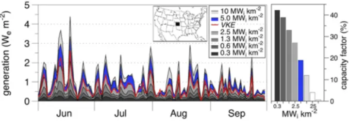
As shown in Fig. 1, the WRF simulations show that a greater installed capacity within the wind farm region increases the total electricity generation rate. This increase is almost linear at the lower installed capacities (0.3 MWi·km−2 ≈ 0.13 We·m−2, 0.6 MWi·km−2 ≈ 0.24 We·m−2; subscripts i and e refer to the installed capacity and electricity generation, respectively). With further increases in the installed capacity, the marginal return of electricity generation predominantly occurs during higher wind speed periods. Such greater generation rates during windy periods can be seen in the differences between the simulations with 5.0 and 10 MWi·km−2 during the high wind speeds of June, whereas the difference is smaller during the lower wind speeds of August and September. Because the greater generation rates occur during pe-riods that are less frequent, the increase in generation is no longer linear. This is reflected by comparing the generated electricity of the 5.0 MWi·km−2to the 0.3 MWi·km−2 simulation, which generates
seven times more electricity with 16 times as many wind turbines. Stated differently, each wind turbine at 5.0 MWi·km−2 generates electricity at half the rate as wind turbines with the same technical specifications but installed at 0.3 MWi·km−2.
This difference in the relationship between generation rate and installed capacity is reflected in a change in the capacity factor. First, we use the hub-height wind speeds of the control simulation and the turbine power curve for the Vestas V112 turbine (SI Appendix, Fig. 6) to calculate the generation rate of a single isolated wind turbine deployed to each location and time. This yields a capacity factor of 47%, which represents the upper bound value for the case of no interactions between the wind tur-bines and the atmospheric flow. This estimate compares well to the capacity factors of 22–36% (1, 7) derived from installed capacity and operational generation data from Kansas during 2006–2012, even though this estimate includes turbines of various technical specifications taken over a much longer timescale than this study. Using the 2012 installed capacity of 2,713 MWi(7) and the area of
213,000 km2 for Kansas yields a state-scale installed capacity of
Fig. 1. (Left) Simulated daily mean electricity generation rates over the Kansas wind farm region (black square on map) for different installed ca-pacities of up to 10 MWi·km−2. The higher installed capacities of 25 and
100 MWi·km−2are not shown, because they often yield less than the 10 MWi·km−2
simulation. For comparison, the VKE estimate is shown in red. (Right) The mean per-turbine capacity factor derived for the different simulations.
0.013 MWi·km−2, which falls below the lowest installed capacity
that we used. Our simulation with the lowest installed capacity of 0.3 MWi·km−2corresponds to a slightly reduced capacity factor of 42%, and 39% with 0.6 MWi·km−2(SI Appendix, Table 2). These capacity factors compare well with the previously used values for this region of 37% (6) and 40–47% used by the Na-tional Renewable Energy Laboratory (7). However, the estimates of refs. 6 and 7 used an installed capacity of 5.0 MWi·km−2, which in our simulations yield a much lower capacity factor of 19%, which should thus result in much lower estimates for wind power generation.
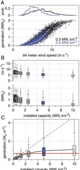
The reduction in capacity factor with greater installed capacity results from an enhanced interaction of wind turbines with the atmospheric flow. Because a greater installed capacity of wind turbines removes more kinetic energy from the atmosphere and converts it into electric energy, this causes a decrease in the hub-height wind speed downwind (26), which decreases the mean per-turbine electricity generation rate of the wind farm. This re-duction in wind speeds within the wind farm and its effects on the per-turbine electricity generation rate is shown in Fig. 2 in re-lation to the power curve of the turbine and the wind speed histogram (Fig. 2A) as well as the mean wind speed and mean per-turbine generation rate (Fig. 2B). The point spread around the 3.0 MWiturbine power curve in Fig. 2A, with some values below the 3.0 m·s−1cut-in wind speed, is due to the use of mean
hourly hub-height wind speed and electricity generation rate for the entire wind farm region. Additionally, the variability in hub-height wind speed decreases with greater installed capacity (Fig. 2B), which also decreases the variability of per-turbine electricity generation. This reduction in wind speeds has also been observed in previous modeling studies (9–12, 27, 28).
Fig. 2C shows the increasing importance of considering the reduction in wind speed for the mean generation rate of the wind farm with greater installed capacity. The dashed line in Fig. 2C is derived by applying the turbine power curve to the control hub-height wind speeds for a mean per-turbine capacity factor of 47% (slope = 0.47). The WRF simulations with installed ca-pacities of less than about 1 MWi·km−2yield similar estimates
because the capacity factors remain high (see alsoSI Appendix, Table 2). At greater installed capacities, the WRF simulations resulted in proportionally lower estimates. For example, at an installed capacity of 2.5 MWi·km−2the“no interactions” estimate would yield a generation rate per unit area of the wind farm of 1.18 We·m−2, but this was simulated to be 0.68 We·m−2. This dis-crepancy continues with greater installed capacities, so at 5.0 MWi·km−2 the estimate without interactions overestimates the average electricity generation rate by more than a factor of two (2.4 We·m−2for no interactions, 0.95 We·m−2with interactions). The maximum electricity generation rate of 1.1 We·m−2 is
obtained with an installed capacity of 10 MWi·km−2, at which the
associated hub-height wind speed decreased by 42% and the capacity factor is reduced to 12%. Our WRF simulations suggest that previous estimates of mean wind energy generation poten-tials for Kansas of 1.9 We·m−2 (6), 2.0–2.4 We·m−2 (7), and
2.5 We·m−2(4) are likely to be too high because the effects of
reduced wind speeds were not considered. To place this reduction into the context of present-day wind power deployment, note that such installed capacities are several orders of magnitude larger than presently operational Kansas wind farms. Our simulations thus suggest that an equidistant deployment of 50 times more installed wind power in Kansas than is presently operational (≈ 0.013– 0.6 MWi·km−2) would maintain the presently high per-turbine capacity factors and thus increase the generation rate 50-fold.
The VKE method captures the magnitude of wind power gen-eration as well as its temporal variations. In our Kansas scenario, we estimate a maximum 4-mo mean generation rate from WRF at 10 MWi·km−2as 1.1 We·m−2and VKE as 0.64 We·m−2. Based on the
linear correlation, the daily mean estimates of the two methods are
highly correlated: r2= 0.98, with a slope of m = 1.76, an rmse of 0.60, and a mean absolute error (MAE) of 0.47. The WRF estimate from the 5.0 MWi·km−2simulation, an installed capacity often used for wind power planning and policy analysis (6), also compares very well, with daily mean estimates being highly correlated with VKE with r2= 0.98, m = 1.47, rmse = 0.39, and MAE = 0.32. The mean
generation rate of this WRF simulation was 0.95 We·m−2, nearly the
same rate as the 10 MWi·km−2 simulation, but from half the number of turbines. When hourly estimates of WRF and VKE are compared (Fig. 3), we note that correlations are very high during day and night, but the slope is much better captured by VKE during the day, whereas at night VKE underestimates the magnitude of electricity generation by almost 45% in this simulation.
Fig. 2. (A) The per-turbine electricity generation rate for two select WRF simulations as a function of hub-height wind speed at 84 m as well as its histogram (Top). The dashed line shows the Vestas V112 3.0 MWipower
curve of a single turbine. (B) Mean per-turbine generation rate and the 84 m mean hub-height wind speed of the wind farm region as a function of in-stalled capacity. (C) Mean per-turbine electricity generation rate as a func-tion of installed capacity when the capacity factor of a single turbine is extrapolated to high installed capacities (dashed line,“no interactions”) and the relationship derived from the WRF simulations (solid line,“interactions”). The red line shows the VKE estimate. All box-whisker plots show the 5, 25, 50, 75, and 95% values, with the extent showing the minimum–maximum and the circles showing the mean.
APPLIED
PHYSICAL
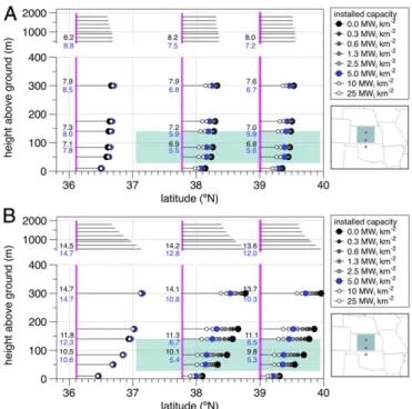
We attribute this underestimation of wind power generation by VKE at night to its use of the preturbine downward kinetic energy flux of the control. The atmospheric flow in this region typically decouples from the stable surface conditions at night in the summer, which leads to the formation of the low-level jet (LLJ) near the surface (29). The typical nighttime structure of the LLJ (Fig. 4B) with a mean stable boundary layer height of 40 m (12–124 m, 5th–95th percentile, respectively) from June– September 2001 in the WRF control mean is consistent with height observations of about 50–350 m in southeastern Kansas during October 1999 (30). Observed LLJ maxima at about 100 m after sunset with an increase in height to about 225 m over the course of the night were also observed for this region on October 25, 1999 (30). The rotors of the wind turbines extend from 28 to 140 m in height and thus reside above, within, or at the upper boundary of the stable boundary layer. The wind turbines in the WRF simulations can thus sometimes directly use the kinetic energy from above the constant stress layer and the LLJ at night. This increased utilization of kinetic energy of the LLJ and the flow of the free atmosphere results in an increased downward kinetic energy and thus a greater maximum generation rate in WRF compared with the VKE method, which does not account for this effect. Based on the nighttime hourly mean values for the wind farm region, a hub-height speed of 9.5 m·s−1and a surface
momentum flux of 0.15 kg·m−1·s−2 yields a downward kinetic
energy flux of 1.39 W·m−2with an associated maximum
gener-ation rate of 0.36 We·m−2by VKE. Daytime atmospheric con-ditions are different. The daytime mean convective boundary layer height in the WRF control simulation is 1,268 m. Of this total height, the constant stress layer, the vertical depth over which the downward kinetic energy flux is considered negligible, typically constitutes the lowest 10% of the convective boundary layer (31, 32). Therefore, during the daytime, the upper extent of the turbine rotors is likely to be within the constant stress layer. Based on mean daytime values, a hub-height speed of 6.9 m·s−1
and a surface momentum flux of 0.37 kg·m−1·s−2 yields a
downward kinetic energy flux of 2.55 W·m−2with an associated
maximum generation rate of 0.65 We·m−2by VKE. Note how the
daytime VKE estimate is about double the nighttime estimate, even though the wind speed during the daytime is lower. These differences between the nighttime and daytime downward ki-netic energy fluxes also help explain the similarities and dis-crepancies between the daytime and nighttime VKE and WRF estimates (Fig. 3).
One last point to note is that the maximum mean electricity generation rate of 1.1 We·m−2 achieved in WRF has notable
effects on the atmosphere and would likely induce considerable differences in climate. Although several recent studies evaluated how wind power generation caused climatic differences in mea-surements (33, 34) and modeling (10, 12, 13, 27, 35–37), the
reduction of wind speeds is relevant here, because this reduction sets the large-scale limit to wind power generation. The mean hub-height wind speed in the 10 MWi·km−2 decreased by 42% com-pared with the control (Fig. 2B). This decrease is consistent with VKE, which provides an analytic expression for the decrease in wind speed at maximum generation ofð1 −pffiffiffi3=3Þ · v0= 42%. As described above, it is this decrease in wind speed with greater ki-netic energy extraction by more wind turbines that limits the wind power generation at large scales. That VKE reproduces the de-crease inv0very well is likely the reason why it captures the mag-nitude and temporal dynamics of limits to large-scale wind power generation of the WRF simulation.
Interpretation
Our estimates from both methods are compared with several other recent studies in Fig. 5. There is a clear discrepancy between esti-mates based on climatological wind speeds (black symbols) from estimates derived with atmospheric models (colored symbols), which are generally lower. We attribute these discrepancies to the inclusion of turbine–atmosphere interactions in the case of the at-mospheric models that result in the reduction of wind speeds in the wind farm. However, one study included in Fig. 5 was derived from existing operational wind farms and observed generation rates, which calls for a more detailed explanation of the discrepancy be-tween those and our estimates. Numerous footprints of operational wind farms in the United Kingdom were digitized (38) and com-pared with their documented generation rate, thereby inherently including turbine–atmosphere interactions. With the majority of the wind farms used in ref. 38 covering relatively small areas of about 2.4 km2(0.1–13 km2) of“footprint area” in hilltop or offshore lo-cations, the wind farms have a mean generation rate of about
1:1 all: r2=0.90, m=1.35, rmse=0.48 a 0 90,, 35,, se 0 8 night: r2=0.92, m=1.79, rmse=0.56 day: r2=0.92, m=1.23, rmse=0.41 WRF (W e m -2) VKE (We m-2) 0 1 2 3 4 5 0 1 2 3 4
Fig. 3. Comparison of hourly mean electricity generation rates for the wind farm region estimated by VKE and WRF with an installed capacity of 5 MWi·km−2.
Fig. 4. Mean (A) daytime and (B) nighttime wind speeds for three selected locations across the wind farm region (Inset) for the control and seven WRF simulations with different installed capacities with one location generally upwind and two locations within the wind farm region. The teal boxes show the spatial and vertical extent of the wind farm. The pink bars and dots show the spatial locations where the mean wind speeds were taken. Wind speeds at the hub height of 84 m and top-of-rotor height of 140, 300, and 500 m for the three locations are noted as text for the control (black numbers) and 5.0 MWi·km−2(blue numbers). Note the break in both y axes.
2.9 We·m−2(0.8–6.6 We·m−2) from a mean installed capacity
of about 11 MWi·km−2(3.5–24 MWi·km−2). These generation rates are substantially higher than our 1.1 W·m−2 limit of
large-scale wind power generation in Kansas, although the size of the wind farms is also notably smaller.
This difference in wind power generation rates can be understood by relating the kinetic energy used by the wind turbines to their sources. For this, we distinguish between the import of kinetic en-ergy by horizontal and vertical fluxes into the wind farm region. These two contributions change as the spatial scale of the wind farm increases. This change can be illustrated by using the mean values of the wind farm region from the WRF control simulation over the 4-mo period. The mean horizontal flux of kinetic energy is given by KEin,h= ð1=2Þρv30· x · h, where ρ = 1.1 kg·m−3 is the air density at hub height,v0= 8.0 m·s−1 is the hub-height wind speed at 84 m, x = 360,000 m is the east–west extent of the wind farm that is per-pendicular to the mean wind direction, andh = 112 m is the height of the wind farm, assumed here to be equivalent to the rotor di-ameter of the 3.0 MWiturbine. This yields a mean horizontal ki-netic energy flux ofKEin,h= 11 GW (or 282 W·m−2per unit cross-sectional area) into the upwind vertical cross-section of the wind farm region. The mean vertical kinetic energy flux is given by KEin,v= ρu2*· v0· x · y, where the mean (spatial and temporal) fric-tion velocity at the surfaceu* = 0.45 m·s−1andy = 312,000 m is the north–south extent of the wind farm that describes the downwind length of the wind farm. This yields a mean vertical kinetic energy flux downward into the entire wind farm region ofKEin,v= 200 GW or 1.8 W·m−2per unit surface area of the wind farm region, so that
in the Kansas setup,KEin,vprovides about 20 times as much kinetic energy as the horizontal influx. Note that this vertical flux of kinetic energy, derived from the WRF control simulation, served as the input to the VKE estimate. When the wind farm increases in downwind length with a greater value ofy, the contribution by the vertical kinetic energy flux into the wind farm region increases lin-early whereas the horizontal contribution remains relatively un-changed. WRF simulations with an installed capacity of 1 MWi·km−2
or greater (>110 GWi) represent wind farms in which the installed
capacity is of the order of the mean kinetic energy flux into the wind farm region (about 211 GW), which is when the reductions of wind speed start to play a role in shaping the generation rate.
In the context of the Kansas wind farm region, we can use these considerations to estimate the downwind depth at which the horizontal kinetic energy flux is fully consumed by electricity generation and turbulence. Assuming a conservative 33% loss to turbulence during the extraction process (25), the 11-GW mean horizontal kinetic energy flux would result in a maximum elec-tricity generation rate of 7.4 GWe. This generation rate is equivalent to about 5,800 wind turbines of 3.0 MWicapacity with a 42% capacity factor, which is close to our WRF simulation at the lowest installed capacity of 0.3 MWi·km−2. When considering
the much greater installed capacity of 5.0 MWi·km−2, the 11 GW
of horizontal kinetic energy flux would be fully consumed within a downwind depth of about 10 km (see also ref. 22). Therefore, as the downwind extent of the wind farm grows, electricity gen-eration rates of successive downwind turbines are derived pro-gressively less from the horizontal flux and more from the vertical flux. This results in an edge effect of higher generation rates at the upwind border of the wind farm compared with lower generation rates in the interior of the wind farm region (see also SI Appendix, Fig. 9). This edge effect does not exist for the VKE estimate (SI Appendix, Fig. 9), because it neglects the horizontal kinetic energy flux as an energy source. This can in part explain the lower estimates of the VKE method. However, when con-sidering wind farms of greater sizes, the influence of this edge effect on the mean generation rate becomes progressively less important to consider.
Generation rates above those estimated by VKE could be achieved if the incoming horizontal kinetic energy flux is avail-able to the wind farm because it was not extracted by upwind turbines, or relate to an increase in the vertical kinetic energy flux by the wind turbines, as shown to particularly occur in the WRF simulations at night. The spatial extent over which this enhanced vertical kinetic energy flux can be maintained, how much it alters the LLJ, and possibly how this results in a regional redistribution in this flux remain as open questions.
An overall increase in the downward kinetic energy flux at larger deployment scales seems unlikely to occur, because cli-mate model simulations performed at continental and global scales do not predict such an increase for present-day radiative forcing conditions (10, 13). Although these studies did not in-clude a full analysis of the energetics, their predictions broadly agree with the predictions of the VKE method in terms of a maximum of 25–27% of the natural dissipation rate that could be used for electricity generation (10) and a slowdown of hub-height wind velocities by 51% globally, 50% over land, and 51% over the ocean (13). Despite its lack of considering changes in the downward kinetic energy flux, it would nevertheless seem that the VKE method is suitable to provide first-order estimates of the magnitude of wind power generation by large wind farms, but this would require further confirmation.
This agreement does not resolve the apparent discrepancy between our estimates and the observation-based estimates from small UK wind farms (38); note that these wind farms have downwind depths much less than 10 km, making their electricity generation rates almost exclusively dependent on the horizontal kinetic energy flux. Formulated differently, edge effects determine the generation rate of these small wind farms. To illustrate com-patibility with WRF-simulated results, we apply the footprint area definition of ref. 38 for isolated 3.0 MWiwind turbines (i.e., a circle with diameter five times the turbine diameter, or 0.25 km2 per turbine) to our simulation of 0.3 MWi·km−2. This results in each
3.0 MWiturbine being spaced 3.1 km apart and yields a comparable
electricity generation with interactions (W e m -2)
electricity generation without interactions (We m-2) this study using WRF
this study using VKE Keith et al. (2004) Miller et al. (2011), T42 Jacobson & Archer (2012) Adams & Keith (2013)
Archer & Jacobson (2005) Lopez et al. (2012)
Jacobson & Delucchi (2011)
1:1 NREL (2012) MacKay (2013) Lu et al. (2009) Lu et al. (2009) 0.1 1 10 100 0.1 1 10 100
Fig. 5. Regional (squares) and continental-to global scale (circles) large-scale electricity generation esti-mates in relation to the effect of turbine–atmosphere interactions. The estimates represented by black squares and circles used preturbine wind speeds without including turbine–atmosphere interactions and are placed on the 1:1 line for reference. The col-ored points refer to estimates based on atmospheric models. These estimates simulate wind speeds and in-clude turbine–atmosphere interactions (y axis). The value on the x axis was derived from using the turbine power curve, installed capacity, and the wind speeds of the control simulation. The horizontal line at 0.64 We·m2with interactions is the VKE estimate for
Kansas (based on figure 4 from ref. 12 with additional studies and the VKE estimate added).
APPLIED
PHYSICAL
5.1 We·m−2for the turbines. For progressively larger installed
ca-pacities, this estimate decreases to 4.7 We·m−2for an installed
ca-pacity of 0.6 MWi·km−2, to 4.0 We·m−2 for 1.3 MWi·km−2, to 3.3 We·m−2for 2.5 MWi·km−2, to 2.3 We·m−2for 5.0 MWi·km−2, and to 1.3 We·m−2for 10 MWi·km−2.
In summary, these considerations illustrate the strong de-pendence of small-scale wind farms on a horizontal kinetic en-ergy flux that is not influenced by other wind farms upwind. Our results suggest that expanding wind farms to large scales will limit generation rates by the vertical kinetic energy flux, thereby con-straining mean large-scale generation rates to about 1 We·m−2even in windy regions. Large-scale estimates that exceed 1 We·m−2thus
seem to be inconsistent with the physical limits of kinetic energy generation and transport within the Earth’s atmosphere.
Conclusion
We evaluated large-scale limits to wind power generation in a hypothetical scenario of a large wind farm in Kansas using two distinct methods. We first used the WRF regional atmospheric model in which the wind farm interacts with the atmospheric flow to derive the maximum wind power generation rate of about 1.1 We·m−2. This maximum rate results from a trade-off by which a greater installed capacity resulted in a greater reduction of wind speeds within the wind farm. This reduction in wind speeds reflects the strong interaction of the wind farm with the atmo-spheric flow, with speeds reduced by 42% at the maximum generation rate. We then showed that these estimates can also be derived by the VKE method, which used the downward influx of kinetic energy of the control climatology and its partitioning into turbulent dissipation and wind-energy generation as a basis. The
VKE method predicts that the maximum generation rate equals 26% of the instantaneous downward transport of kinetic energy through hub height. This method only required the information of wind speeds and friction velocity of the control climate to provide an estimate of a maximum wind power generation rate. With an estimate of 0.64 We·m−2, the VKE method underestimates the maximum wind power generation rate, particularly during night, but it nevertheless captures the temporal dynamics as well as the re-duction in wind speeds very well.
Both methods used here yield estimates for the limits to large-scale wind power generation that are energetically consistent. Although many current wind farms are still comparatively small and can therefore sustain greater generation rates, an energeti-cally consistent approach becomes relevant when the installed capacity of the wind farm approaches the kinetic energy flux into the wind farm region. Although the VKE method assumes this influx to be fixed, it nevertheless demonstrates that an energetically consistent estimate can be done in a comparatively simple way, thus providing a useful means to derive a first-order estimate of large-scale wind power generation from preturbine climatologies. We conclude that large-scale wind power generation is thus limited to a maximum of about 1 We·m−2because of this inevitable reduction of
wind speeds and the comparatively low vertical kinetic energy fluxes in the atmosphere.
ACKNOWLEDGMENTS. We thank C. Dhara, M. Renner, N. Carvalhais, two anonymous reviewers, and the editor for their suggestions and constructive comments that helped improve the mansucript. This study was funded by the Max Planck Society through the Max Planck Research Group of A.K. A.J.M. was funded by the National Science Foundation.
1. US Energy Information Administration (2014) Annual energy review. Available at www.eia.gov/totalenergy/data/monthly/. Accessed July 28, 2015.
2. Wiser R, Bolinger M (2012) 2011 Wind technologies market report.US Department of Energy, Energy Efficiency & Renewable Energy report DOE/GO-102012-3472 (US De-partment of Energy, Oak Ridge, TN).
3. Archer C, Jacobson M (2005) Evaluation of global wind power. J Geophys Res 110(D12):D12110.
4. Lu X, McElroy MB, Kiviluoma J (2009) Global potential for wind-generated electricity. Proc Natl Acad Sci USA 106(27):10933–10938.
5. Jacobson MZ, Delucchi M (2011) Providing all global energy with wind, water, and solar power, Part I: Technologies, energy resources, quantities and areas of
in-frastructure, and materials. Energy Policy 39:1154–1169.
6. Lopez A, Roberts B, Heimiller D, Blair N, Porro G (2012) U.S. renewable energy technical potentials: A GIS-based analysis. US Department of Energy National Re-newable Energy Laboratory report TP-6A20-51946 (US Department of Energy, Golden, CO).
7. National Renewable Energy Laboratory (2012) Stakeholder engagement and outreach. Available at apps2.eere.energy.gov/wind/windexchange/pdfs/wind_maps/ wind_potential.pdf and apps2.eere.energy.gov/wind/windexchange/wind_installed_ capacity.asp. Accessed May 2, 2014.
8. Gustavson MR (1979) Limits to wind power utilization. Science 204(4388):13–17. 9. Keith DW, et al. (2004) The influence of large-scale wind power on global climate.
Proc Natl Acad Sci USA 101(46):16115–16120.
10. Miller LM, Gans F, Kleidon A (2011) Estimating maximum global land surface wind power extractability and associated climatic consequences. Earth Syst. Dynam 2:1–12.
11. Gans F, Miller LM, Kleidon A (2012) The problem of the second wind turbine— a note
on common but flawed wind power estimation methods. Earth Syst. Dynam 3:79–86. 12. Adams AS, Keith D (2013) Are global wind power resource estimates overstated?
Environ Res Lett 8:015021.
13. Jacobson MZ, Archer CL (2012) Saturation wind power potential and its implications
for wind energy. Proc Natl Acad Sci USA 109(39):15679–15684.
14. Kirk-Davidoff D (2013) Plenty of wind. Nat Clim Chang 3:99–100.
15. Skamarock WC, et al. (2008) A description of the advanced research WRF version 3.
NCAR technical note NCAR/TN-475+STR (National Center for Atmospheric Research,
Boulder, CO).
16. Wang W, et al. (2012) WRF ARW V3: User’s Guide (National Center for Atmospheric Research, Boulder, CO).
17. Mesinger F, et al. (2006) North American Regional Reanalysis. Bull Am Meteorol Soc 87:343–360.
18. Trier S, Davis C, Ahijevych D (2009) Environmental controls on the simulated diurnal cycle of warm-season precipitation in the continental United States. J Atmos Sci 67: 1066–1090.
19. Fitch A, Olson J, Lundquist J (2013) Parameterization of wind farms in climate models. J Clim 26:6439–6458.
20. Calaf M, Meneveau C, Meyers J (2010) Large eddy simulation study of fully developed wind-turbine array boundary layers. Phys Fluids 22:015110-1–015110-16.
21. Meyers J, Meneveau C (2012) Optimal turbine spacing in fully developed wind farm boundary layers. Wind Energ. 15:305–317.
22. Meneveau C (2012) The top-down model of wind farm boundary layers and its
ap-plications. J Turbul 13:1–12.
23. Garrett C, Cummins P (2007) The efficiency of a turbine in a tidal channel. J Fluid
Mech 588:243–251.
24. Garrett C, Cummins P (2013) Maximum power from a turbine farm in shallow water. J Fluid Mech 714:634–643.
25. Corten G (2001) Novel views on the extraction of energy from wind: Heat generation and terrain concentration. Proceedings of the 2001 EWEC conference. Available at www.ecn.nl/docs/library/report/2001/rx01054.pdf. Accessed May 2, 2014.
26. Iungo G, Wu Y, Porté-Agel F (2013) Field measurements of wind turbine wakes with lidars. J Atmos Ocean Technol 30:274–287.
27. Miller LM, Gans F, Kleidon A (2011) Jet stream wind power as a renewable energy resource: Little power, big impacts. Earth Syst. Dynam 2:201–212.
28. Fitch A, et al. (2012) Local and mesoscale impacts of wind farms as parameterized in a mesoscale NWP model. Mon Weather Rev 140:3017–3038.
29. Blackadar A (1957) Boundary layer wind maxima and their significance for the growth of nocturnal inversions. Bull Am Meteorol Soc 38(5):283–290.
30. Pichugina Y, Banta R (2009) Stable boundary layer depth from high-resolution
measurements of the mean wind profile. J Appl Meteorol Climatol 49:20–35.
31. Driedonks A, Tennekes H (1984) Entrainment effects in the well-mixed atmospheric
boundary layer. Boundary-Layer Meteorol 30(1-4):75–105.
32. Stull R (1988) An Introduction to Boundary Layer Meteorology (Springer, Berlin), Vol 13. 33. Baidya Roy S, Traiteur JJ (2010) Impacts of wind farms on surface air temperatures.
Proc Natl Acad Sci USA 107(42):17899–17904.
34. Zhou L, et al. (2012) Impacts of wind farms on land surface temperatures. Nat Clim Chang 2:539–543.
35. Kirk-Davidoff D, Keith D (2008) On the climate impact of surface roughness anoma-lies. J Atmos Sci 65:2215–2234.
36. Fiedler B, Bukovsky M (2011) The effect of a giant wind farm on precipitation in a regional climate model. Environ Res Lett 6:045101.
37. Vautard R, et al. (2014) Regional climate model simulations indicate limited climatic impacts by operational and planned European wind farms. Nat Commun 5:3196. 38. MacKay DJ (2013) Could energy-intensive industries be powered by carbon-free
electricity? Philos Trans A Math Phys Eng Sci 371(1986):20110560.