HAL Id: hal-02301063
https://hal.archives-ouvertes.fr/hal-02301063
Submitted on 30 Sep 2019HAL is a multi-disciplinary open access archive for the deposit and dissemination of sci-entific research documents, whether they are pub-lished or not. The documents may come from teaching and research institutions in France or abroad, or from public or private research centers.
L’archive ouverte pluridisciplinaire HAL, est destinée au dépôt et à la diffusion de documents scientifiques de niveau recherche, publiés ou non, émanant des établissements d’enseignement et de recherche français ou étrangers, des laboratoires publics ou privés.
Spatial aggregation methods: an interactive
visualization tool to compare and explore automatically
generated urban perimeters
Laurent Jégou, F. Bahoken, Emna Chickhaoui, Étienne Duperron, Marion
Maisonobe
To cite this version:
Laurent Jégou, F. Bahoken, Emna Chickhaoui, Étienne Duperron, Marion Maisonobe. Spatial ag-gregation methods: an interactive visualization tool to compare and explore automatically generated urban perimeters. 59th ERSA Congress ”Cities, regions and digital transformations: opportunities, risks and challenges”, Aug 2019, Lyon, France. �hal-02301063�
Spatial aggregation methods: an interactive visualization tool to compare and explore automatically generated urban perimeters
Authors:
Laurent Jégou, geographer, Univ. Toulouse-2 and UMR LISST/Cieu
Françoise Bahoken, geographer, researcher at Université Paris-Est / AME-SPLOTT / IFSTTAR & ass. UMR Géographie-Cités / PARIS
Emna Chickhaoui, student, Master Sigma, Univ. Toulouse-2 Étienne Duperron, student, Master Sigma, Univ. Toulouse-2
Marion Maisonobe, geographer, researcher at CNRS, UMR Géographie-Cités
Abstract
Choosing the appropriate scale of analysis is a well-known problem in regional studies. Changing the level of spatial analysis is not trivial and can have substantial effects on the resulting the indicators, their representation and their interpretation, especially if the original data is spatially diverse and at a fine granularity. One cannot regroup locational data as spatial data points automatically without consequences. As geographical datasets are becoming increasingly available, with a finer resolution, and as territorial / spatial clustering algorithms are becoming easier to apply on vast amounts of spatial data, we want to provide a geospatial application, which could help to present and analyse this issue. What definitions can be used to delineate the idea of a city, an urban area or an agglomeration? At what size, population density, volume of urban activity or surface are we observing a city? We consider this issue especially in a methodological comparative purpose taking the example of analysing the volume of scientific activity of European cities.
In this proposal, we provide a comparative analysis of spatial clustering methods or aggregation procedures. In support of the presentation, we propose an interactive web-based application designed to explain and (geo)visualize their effects on different results: volume of urban activity (discrete values) and city rankings (ordinal values), on the one hand; and effects on the spatial configuration, on the other hand. In this exploratory work, we will focus on functional data about the geography of scientific production. To delineate automatically functional perimeters of European cities, we use the distribution of scientific activities i.e. the number of publications per municipalities computed from the Web of Science database following an extensive process of geo-localisation of authors’ addresses (Eckert et al., 2013). We will compare the results of several spatial aggregation methods applied on these geolocalized points: Hierarchical Clustering using various aggregation functions and criteria with or without weighting, then density-based methods including DBSCAN and HDBSCAN. We will use the volume of scientific publications associated to each geolocalized points as a weighting indicator.
Introduction
What is a city? In geography, the definition of the key-concept of city is not given, it is sensitive especially to the way in which geography – in the terms of positions of places in space - is considered: as a continuous surface and/or as an assemblage of discrete entities. On a continuous geographical space, what is the delineation that encloses enough content to allow thinking of it as a city? What if one changes the scale of analysis, from regional to international? In a discrete approach, from when does a city is symbolized by a single data point or a geometric surface?
This question is at the core of urban geography and regional studies. For a long time, measures were collected and statistics were produced according to political-administrative divisions or dedicated territorial frameworks. This means that they were carried out within, firstly, existing territorial partitions and, secondly, the framework of a discrete approach. The problem with this approach is that such partitions of the geographical space - by definition continuous - into distinct areas are exclusive (a geographical object belongs to one and only one class) and more or less heterogeneous. These divisions were often used by default by analysts from the 19th century until the late 1960s, the early 1970s, and before the so-called spatial turn.
This bias is important to take into account when one hopes to compare data spatially and study flows between locations. Various authors in demography, economy and geography, have been able to demonstrate the binding role of such political-administrative divisions in the implementation of geographical or economic models, in particular those concerning the analysis of spatial interactions (Alvanides et al., 2000). For a recent theoretical and methodological review applied to relational data (links or flows), see Van Hamme & Grasland (2011). Some authors have proposed partition methods based on relational data that ignore administrative divisions such as methods that maximize/minimize cumulated intra-zonal interactions. In the specific case where links data are used as methods of partitioning geographic space, what is important is the choice of the aggregation function, taking into account its effects (Masser & Brown, 1975; Hirst, 1977). Similarly, the instability of statistical results in the context of a variable geographical unit (better known as the Modifiable Area Unit Problem - MAUP) is proven (Openshaw, 1977). These problems are acute, particularly at the international and global scale - which is already sensitive to the choice of the mapping projection system: first, administrative areas are not designed to delineate functional areas and, second, they are not easily comparable between countries. As geographical datasets are becoming increasingly available, with a finer scale and local data points, this issue is particularly relevant.
Concretely, the questions that we need to address are:
1) Should we consider the geographic space as a discrete partition where cities are points or areas (depending on the scale)? Alternatively, should we consider it as a (continuous) surface where cities are defined by a scope with potentially fuzzy boundaries?
2) How to associate local data points into meaningful aggregations, adjusted to the analysis, called clusters or functional regions? The effects of unadapted clustering methods can be quite elusive to the researcher, due to their complexity and subtle variations, particularly spatial ones. Actually, the spatial component of the problem weighted or not, combined with the different scales of analysis and the exploration of relative values and flows can rapidly muddle the situation.
With this contribution, we want to provide an update on the issue, to expose the main methods of spatial clustering and, more particularly, to illustrate the effects of varying parametrization on the face of a map. We would also like to explore these variations graphically, by proposing several innovative interactive representations. Indeed, we think that a hands-on approach can be useful to describe the issue, increase its awareness and explore the parameter space of several methods and their effects.
Our contribution is organized in three parts. First, we distinguish between two families of spatial clustering methods. Second, we present the R-Shiny application developed for the sake of this comparative research on spatial clustering methods applied to the objective of delineating functional urban areas. Finally, we test and compare clustering methods applied to data points from the point of view of a researcher interested in changing the scale of his or her analysis.
1. Spatial clustering methods: a brief glance
To illustrate the diversity of methods of partitioning geographic space, we distinguish two families of clustering methods: purely geometrical and weighted by various criteria. Indeed, several methods of spatial clustering are only geometrical, that is to say, they only use the relative positions and the spatial density of the data points to regroup them. The second family of methods can take into account weighting and/or spatial parameters such as, 1) the contiguity or spatial continuity in the aggregation process, 2) the intensity of a phenomenon (population, scientific production for example), or 3) the values of networking properties at a global or a local level (as centrality or connectivity) on reticular or flow data.
From the first group, DBSCAN (Ester et al., 1996, Campelo et al., 2013) and its variants are currently being widely used. We will show in a complementary perspective that hierarchical classifications like HCLUST (Müllner, 2013) and AGNES (Kaufman and Rousseeuw, 2009) can also be very effective, with a cautious attention to fine-tune their parameters.
From the second group, we can consider weighted variants of DBSCAN methods as well as weighted extensions of hierarchical classification methods such as HCLUSTGEO (Chavant et al., 2017).
In what follows, we will more specifically compare and test AGNES, HCLUST and HCLUSTGEO that are variants of hierarchical classifications (HCLUST being purely geometrical – 1st family – and HCLUSTGEO being a weighted variant – 2nd family) with a weighted DBSCAN method (2nd family) and the non-weighted DBSCAN and HDBSCAN methods. In so doing, we will attempt to confirm and highlight the efficiency of hierarchical classifications for spatial clustering as suggested by Chikhaoui and Duperron in the Master Report they produced in 2019 under our supervision on this specific issue (Chikhaoui and Duperron, 2019). More advanced methods belonging to the second family of algorithms will be considered at a later stage of this ongoing research, as those considering relational data between points or spatial constraints (see Conclusion).
2. An R-Shiny application to compare spatial clustering methods for urban area delineation
The approach we implement in R/Studio and R-Shiny is intended to be generalizable and reproducible (Giraud and Lambert, 2017). This is why we propose to provide all our R algorithms, combined within an R-Shiny application, which provides a friendly user interface for web support visualization.
This proposal is also in accordance with the principle of "muti-cartographic representation" (Zanin and Lambert, 2012), by allowing an interactive exploration and visualization of linked tabular, graphic and cartographic depictions. The R platform offers indeed an interesting collection of tools to analyse data in real time (with specialized clustering modules), and to represent results on interactive maps and graphs.
2.1. Spagreg, a dedicated web application
Our prototype is freely available on the following web link: http://www.geotests.net/spagreg/. It allows selecting an aggregation method, and, when the method is hierarchical, visualizing the result on the corresponding dendrogram (with mention of the agglomerative coefficient). For all methods, it gives access to the cartographic result in an interactive way – by automatically drawing of the limits of the resulting clusters, and to the corresponding data table.
To explore the spatial component of the clustering problem, we choose to display the results on an interactive map of Belgium and the Netherlands. Selecting Belgium and the Netherlands for our case study is justified by the very important population density of this geographical space, which makes difficult the task of delineating distinct functional urban areas within it (Maisonobe, 2015). The points that we offer to cluster correspond to the centroids of the municipalities from where scientific publications indexed in the Web of Science database have been authored between 1999 and 2014. These points were geolocalised by the Netscience research team. Since 2013, this geospatial analysis of scientific production activity is performed at the level of urban areas delineated according to a semi-automatic methodology – the dataset of the urban agglomerations used in this research project has recently been released online (Maisonobe et al., 2018). With the Spareg web application, we explore the opportunity of using entirely automatic clustering methods to generate “scientific agglomerations”.
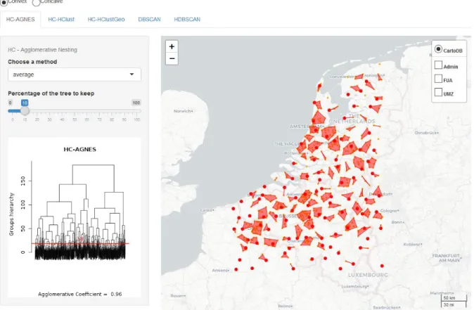
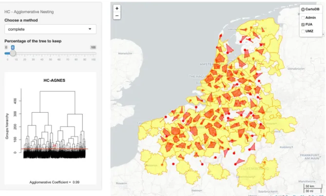
The Spagreg web application thus allows depicting a punctual dataset and presenting the results of several clustering methods by visualizing the clusters’ geographical scopes. It presents the spatial effects resulting from the choice of one spatial clustering method over the other; and it interactively shows the role of tuning the parameters, by redrawing the map in real time (Figure 1).
The red shapes are the resulting clusters of the selected clustering method (HC-AGNES on Figure 1). The small orange dots display the locations of the scientific places that we attempt to cluster. The biggest red point that one can detect within each shape corresponds to the location of the publication spot associated with the highest number of scientific publications, that is to say, the more active scientific spot of the cluster, which we can consider as the centre of the resulting “scientific agglomeration”.
The application let the user choose the type of polygon construction methods to apply to the groups of points constituting the clusters, between convex and concave hulls. Convex hulls are more often used so that the points define the outer perimeter of the clusters. For a more conservative method of polygon creation, concave hulls restrict the polygon surface to the points selected with a smallest distance rules at the outer border, which enables potentially less overlapping between adjoining clusters.
Figure 1. Snapshot of the R-Shiny application displaying clusters generated with the AGNES algorithm
2.2. Interactive display of spatial clustering methods
Left to the map, the parameters of the clustering method are specified with dedicated user interface widgets. With the agglomerative nesting method, AGNES, one can choose the specific clustering method and the percentage of the agglomerative tree to keep. Below the parameters, the user can view the result of the clustering in the classical representation mode of the dendrogram, the kept percentage of which is figured by a red horizontal line (Figure 1).
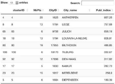
To demonstrate the consequences of the clustering variations on the aggregated end-values, the application presents the table of aggregated values of scientific publications (the resulting number of publications per cluster) – see Figure 2. On this table, one can find below the interactive map, the name of the municipality associated to each cluster corresponds to the name of the most publishing spatial spot (the red point). The associated value (“Publ_indice”) gives the aggregated value (the sum of all the scientific publications attached to the clustered points).
At a later stage of development, the application will also offer the possibility to filter or query the data (to reduce the set or to explore more finely the results) and several graphical representations will be accessible: histograms and more comparative graphs such as Sankeys and bubble charts.
Figure 2. Snapshot of the table displaying the aggregated number of scientific publications per generated cluster – according to the clustering method selected by the application’s user.
The availability of interactive web representations, helped by the development of programming libraries as R modules and JavaScript functions, permit a direct, hands-on interactive exploration of these representations, which helps understanding the reality of the clustering problem and its effects.
To assess the efficiency of these algorithms, one can contrast and compare their results both visually and quantitatively with the resulting clusters values accessible on the interactive table. We also provide the comparison of the results with pre-defined clusters or delineations, such as administrative divisions or functional spatial territories1 created precisely to observe the cities of the European space in a comparative manner ("Functional Urban Areas" by Guérois et al., 2014, and "Urban Morphological Zones" from the ESPON projects2). In particular, we offer to
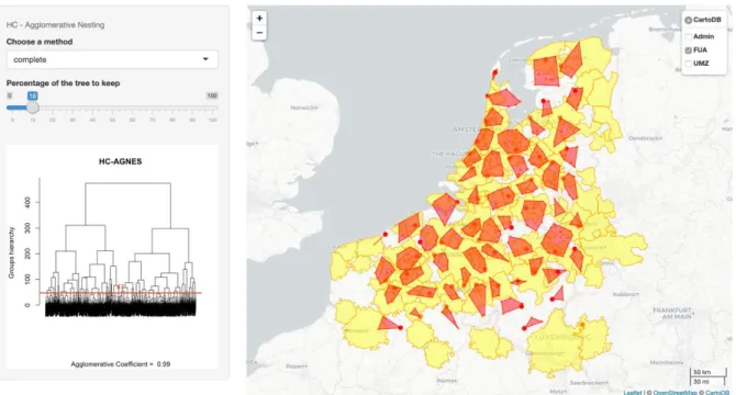
the user the possibility of displaying the delineations of these administrative and functional divisions on the base map – underneath the results of the selected clustering method (see Figure 3).
1 These layers are slightly geometrically generalized, to speed their display, as their use is mainly for visual
comparison.
Figure 3. Snapshot of the map showing AGNES clusters with the Functional Urban Areas as background, for visual comparison.
3. The choice of a clustering method and its effect on the aggregation of data points
To assess the effects of these clustering algorithms on the aggregation of point data, we are using spatial datasets based points (depicting city addresses) with the theme of science production (relying on our complex but interesting dataset about the geography of scientific production). This specific subject, which we are exploring for several years with geocoded data from the Web of Science bibliographical database, is especially interesting due to the surprisingly very recent consideration of the clustering issue in spatial scientometrics and the analysis of networks of scientific collaboration between places (Maisonobe et al., 2018).
By using this example, we aim to demonstrate the harmful effects of dubious clustering decisions, such as the use of administrative divisions to compare the scientific production at a European scale.
Clustering geographical point data is a logical step to analyse the spatial distribution of a phenomenon at a smaller scale. Several existing methods are using different approaches to regroup points, using their longitude and latitude positions and, optionally, quantitative variables. By clustering geographical points, the two main variables, longitude and latitude, are concrete attributes, instead of quantitative proxies. Consequently, the clustering methods using those attributes are geographically well founded and pertinent. Translated into the thematic, if several scientific cities are forming a spatial group distinct from others, their combination into a single cluster is justifiable.
Nevertheless, the different existing methods are using very distinct criteria to qualify the geographical distances and patterns to form clusters; our objective here is to illustrate these differences and their effects on the hierarchy of the produced clusters. We examine these methods in distinguishing two groups, hierarchical and density-based methods.
As described by D. Müllner (2013), these methods are using a progressive hierarchical algorithm to regroup the points into clusters, examining the distance matrix (or dissimilarity matrix) between them:
Start with a number of N singleton nodes.
Find a pair of nodes with minimal distance among all pairwise distances. Join the two nodes into a new node (cluster) and remove the two old nodes.
The distances from the new node to all other nodes is then determined by the “method” parameter (see below).
Repeat N-1 times from step two, until there is one big node (cluster) which contains all the original input points.
The output of this process is called a stepwise dendrogram, showing the progressive groupings as the stems of a tree. When one cut the tree at a certain level, we obtain a corresponding number of clusters (cf. Figure 3, for example).
There are several methods for measuring the distances between the nodes. For the HC-AGNES and HCLUST algorithms implemented in our application, the Rbase offers:
Single: the closest distance between clusters.
Complete: the maximum distance between any two points of the clusters. Average: the average of the distances between the points of the clusters.
Ward: the distance between the points of the clusters are pondered with the distance between their centroids.
Quite evidently, the Euclidean formula is used to calculate the distances, as we are examining geographical locations. For other, more abstract spaces, the algorithms can use other types of distance formulas, as Manhattan’s distance.
AGNES and HCLUST differ by their distance calculation methods and the speed of their algorithms. HclustGeo brings the possibility to use a second data matrix in addition to the spatial dissimilarities and a weighting matrix to factor the Euclidean distance, but only use the Ward criteria to measure distances.
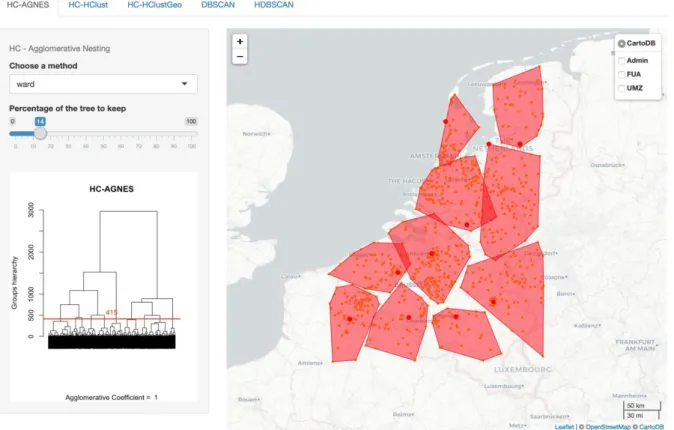
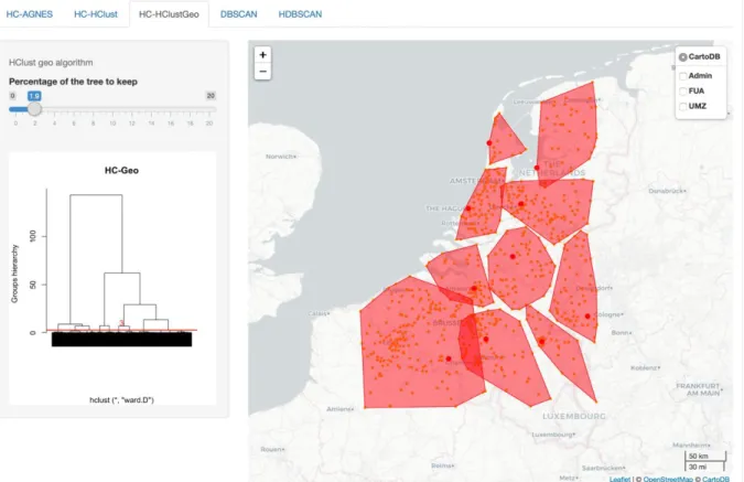
When we use these three algorithms to produce the same number of clusters (10) using the same general distance formula (Ward), the cutting parameter must be different and the results are quite diverse (Figure 4, a, b and c).
Figure 4a: Ten clusters with the AGNES method.
Figure 4c: Ten clusters with the HClustGeo weighted method.
The result of HClustGeo is explainable by the influence of the weighting parameter: one can see that the influence of the Brussels-Leuven region is expanded by its large scientific output. The difference between AGNES and HCLUST, especially in the south and northeast margins of the map, are less easily explainable. We can infer an algorithmic variation perhaps on the dissimilarity matrix use (distances are larger on the margins). Here, we would like to emphasize that the results can be very different, even with the same data and general method. The consequences are especially important when one takes into account the resulting cluster hierarchy: the first two clusters in volume of scientific activity are semblable, but the rest of the ranking varies widely (Figure 5, a, and b).
Figure 5b: hierarchy of the ten clusters created by HClust
When we compare the clusters resulting from a finely tuned method (AGNES, complete distance) with administrative or functional areas, the usefulness of these clustering methods is clear (see Figure 6a, and b). Even by only taking into account the spatial locations of the points, the clusters are different of the reference areas, which suggests a better proximity to the thematic studied.
Figure 6a: Clusters from AGNES-complete method with 6% of the tree, compared with the Functional Urban Areas.
On figure 6a, one can see that the resulting clusters are not aligned with the FUAs. Large metropolitan regions like Brussels contains several clusters, whereas less dense FUAs in the north of the Netherlands are covered by one cluster.
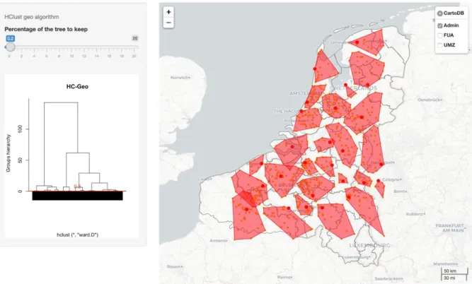
Figure 6b: Clusters from HClutGeo (weighted Ward) method compared with administrative areas.
The contrast is even larger when one compares the clusters with administrative areas. If their center is often the province capital, their extent varies largely and one cluster can cross the boundaries of several provinces.
3.2. Density-based methods
The clustering methods based on spatial density are somewhat gaining traction in recent scientific publications, if we take into account the number of papers refining or expanding the algorithm (on temporal, relational, pixelated data, with neural networks or fuzzy sets for example). They are represented by the variants of the DBSCAN original algorithm (Ester et al., 1996), and especially interesting to the spatial sciences as they are considering the density of points regions instead of relative distances. They measure the connectedness of the points rather than their distance, as are the clustering methods we described earlier.
These methods are more complex than the previous ones, but we can describe them from a general point of view, using the description from A.K. Jain (2010). The DBSCAN algorithm directly looks for connected dense regions in the observed space, by estimating the density using the Parzen moving window method − also known as kernel density estimation. In plain English, the observed points are considered as samples from a continuous spatial distribution function, which is estimated by using probability kernels methods. The more points are in one neighborhood region, the more density is accumulated around this region and the higher is the overall density of the function. The resulting function can be evaluated with a kernel method (often used in geostatistics), for any point.
In our application, we are using the R implementation of DBSCAN and its hierarchical variant, HDBSCAN (from M. Hasler, M. Piekenbrock, and D. Doran). This DBSCAN package provides several code optimizations to speed the calculations. The two variants use the minimal number
of points of the clusters as a central parameter, and the DBSCAN method shows its spatial orientation with a second parameter: the width of the window function, or the radius of the search circle around each node. Interestingly, the method can use a weight matrix to consider a variable in addition to the pure geometrical location of the points. Consequently, the clustering method needs a fine parameter tuning to produce useful results, thus being less automatable.
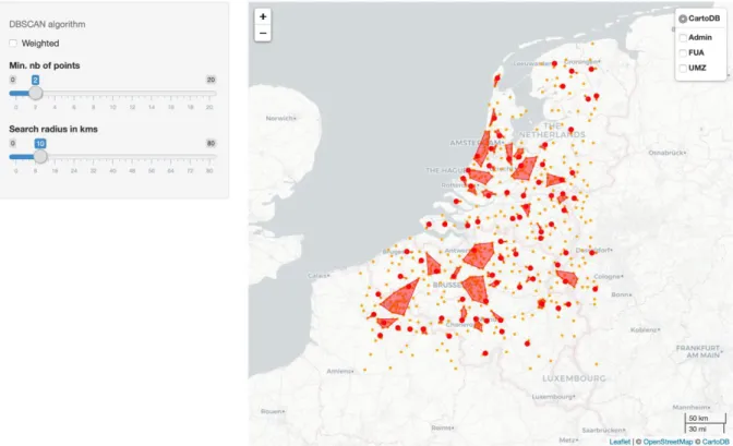
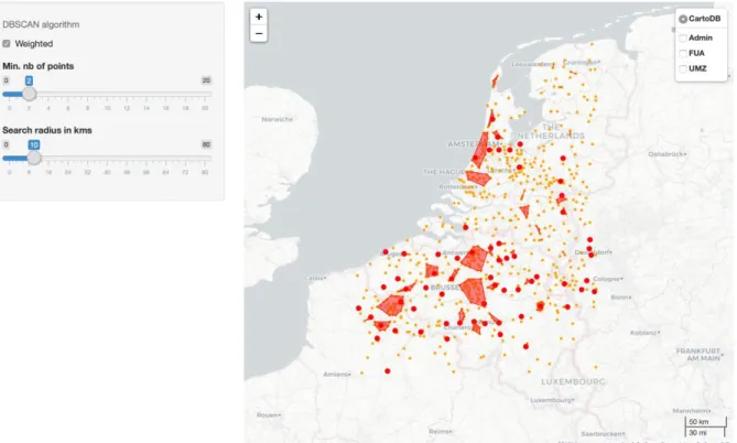
The DBSCAN clustering method, per its algorithms, produce clusters that are largely defined by the spatial densities found on the point space. Indeed, when one chooses a search radius of 10km and the possibility of line clusters (formed by two points only), the resulting map is clearly influenced by the groupings of the points (see figure 7). As DBSCAN is not a hierarchical algorithm, the application does not offer a dendrogram plot. The results are displayed on the map and the clusters table.
Figure 7: DBSCAN method with a 10km search radius.
The comparison with the preceding methods shows very few large clusters and a majority of small ones. Some of the points are not even part of a cluster (orange dots on figure 7). The completely different clustering method generates, as expected, very different clusters and segmentation of the map that is largely not comparable. The DBSCAN method is not adequate to consider heterogeneously dense spaces if one hopes to qualify the totality of the map.
By using the weight of scientific publications, the method produces a small variation of the preceding result (see Figure 8): some clusters nearly disappear (low weights near Bilthoven and Utrecht produce a contraction on a very small cluster) and others are subdivided (around Lille and Kortrijk/Courtrai).
Figure 8: weighted DBSCAN method with a 10km search radius.
The cluster hierarchy are modified consequently, and we detect another difference: with the consideration of the scientific publications as weights, the very small cluster of Julich (Germany) is created (see Figures 9a and 9b). It iss another interesting point of our work: the comparison between the map and the table is fruitful, the effects of the clustering methods are sometimes more legible on the cluster list and hierarchy than on the map. The aforementioned idea that the DBSCAN algorithm tends to produce very heterogenous clusters is maintained with the weighted variant.
Figure 9b: cluster table for non-weighted DBSACN
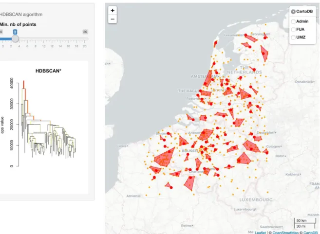
The hierarchical DBSCAN method consists in a hierarchical search of every possible DBSCAN clustering of the points and then uses a stability-based extraction method to find optimal cuts in the hierarchy (from the vignette of the package). It is more complex and takes longer to compute. The only parameter, the minimum point’s number per cluster to produce, is also used as a smoothing factor of the density estimates.
As this last method is a hierarchical method, the output of the R implementation proposes an informative dendrogram plot (see Figure 10). The result of this method, with a parameter of 3 points for the minimal cluster (and as a density smoothing factor), also shows very heterogenous clusters, very like those resulting from a non-weighted DBSCAN algorithm, but with more clusters in medium-dense regions as the east of the map.
4. Conclusion
To conclude our work, we would like to emphasize the usefulness to visualize and compare in an interactive and accessible manner such complex clustering methods. One can explore the parameter space of each method and compare their results in terms of geography of the clusters on the map and their ranking according to a quantitative variable in the table.
By testing these methods on a thematic dataset allowing to study the geography of scientific activities, we have observed that very different spatial perimeters can be generated than by using existing administrative (municipalities’ boundaries) or statistical perimeters (FUAs and UMZs). These automatically generated perimeters are more finely adapted to the studied thematic.
One of the main results of our work is to confirm the very important consequences of the choice of a clustering method and its parametrization. In this matter, our proposal differs from contributions describing existing algorithms as performing and comparable without allowing comparing their results.
On the one hand, the hierarchical methods (AGNES, HClust) seems to provide quite homogenous clusters in terms of size and space covering, their weighted variants help to consider the aggregated value differences between points. On the other hand, the density-based methods (DBSCAN and HDBSCAN) are very much influenced by the spatial distribution of the points, focusing only or especially on the denser groups of points and expunging the more isolated points.
The influence on the spatial representation, as visualized on the map, and on the cluster hierarchy, as visualized on the ranking table, are important. The researcher should carefully test the methods and balance their bias and processing orientations with his or her objectives about the covering of the studied space with clusters. We advise to visualize the results of the possible choices in a comparative way, successively on a map and on a ranking table.
Our prototype application shows promise to expand the possibility of method comparisons and experimentation, especially to non-specialists hoping to test the results on various thematic datasets. Several possibilities of extension exist, especially for generating interactive flowmaps at several geographical level. We can consider, on the one hand the ongoing development of the gFlowiz research program3 and on the other hand, the exploration of the possibility to
combine our datasets with other subjects such as transportation problems including geographical friction and barriers to movements, in a continuous or discrete (e. g. neighbourhoods) forms.
Flows or valued spatial networks studies could benefit from advanced clustering methods based on graph theory that seem promising, like Autoclust+ (Estivill-Castro and Lee, 2004) and ASCDT+ (Liu et al., 2013). Another useful possibility of recent methods is the consideration
of constraints, limits, obstacles and spatial friction or, inversely, easier connection between points and regions, like DBCluc (Zaïane et al., 2002) and DBRS (Wang and Hamilton, 2005).
The possibility for the user to upload his or her own dataset could also be added using the functions of the very efficient and accessible R- Shiny platforms.
Bibliography
Alvanides S., Openshaw S. and Duke-Williams O., 2000, Designing zoning systems for flows data in Atkinson P., Martin D. (eds.), 2000, Geocomputation, Part II: Zonation and Generalization, Taylor & Francis Group, Ed. CRC Press, pp. 115-34.
Chavent M., Kuentz-Simonet V., Labenne A., Saracco J., 2017, ClustGeo: an R package for hierarchical clustering with spatial constraints, arXiv:1707.03897
Chikhaoui, E, Duperron, E., 2019, Recherche et tests d’algorithmes de clustering spatial pour webdataviz, Mémoire de Master SIGMA supervisé par Laurent Jégou et Marion Maisonobe, Université de Toulouse Jean-Jaurès, Toulouse, 73 p.
Campello, R. J. G. B., Moulavi, D.; Sander, J., 2013, Density-Based Clustering Based on Hierarchical Density Estimates. Proceedings of the 17th Pacific-Asia Conference on Knowledge Discovery in Databases, PAKDD 2013, Lecture Notes in Computer Science 7819, p. 160.
Ester M., Kriegel H.-P., Sander J., Xu X., 1996, A Density-Based Algorithm for Discovering Clusters in Large Spatial Databases with Noise. Institute for Computer Science, University of Munich. Proceedings of 2nd International Conference on Knowledge Discovery and Data Mining (KDD-96).
Estivill-Castro, V., and Lee, I., 2004, Clustering with obstacles for geographical data mining. ISPRS Journal of photogrammetry and remote sensing, 59(1-2), 21-34.
Giraud, T., and Lambert, N., 2017, Reproducible Cartography. In: Peterson M. (eds) Advances in Cartography and GIScience. ICACI 2017. Lecture Notes in Geoinformation and Cartography. Springer, Cham.
Guérois, M., Bretagnolle, A., Mathian, H., & Pavard, A., 2014, Functional Urban Areas (FUA) and European harmonization. A feasibility study from the comparison of two approaches: commuting flows and accessibility isochrones (Technical Report, Espon 2013 Database) (p. 35). Paris: Union Européenne.
Hirst M. A., 1977, Hierarchical aggregation procedures for interaction data: a comment, Environment and Planning A, 9(1): 99-103.
Jain, A. K., 2010, Data clustering: 50 years beyond K-means. Pattern recognition letters, 31(8), 651-666.
Kaufman L. and Rousseeuw P. J., 2009, Finding groups in data: an introduction to cluster analysis. Vol. 344: John Wiley & Sons.
Liu, Q., Deng, M., & Shi, Y., 2013, Adaptive spatial clustering in the presence of obstacles and facilitators. Computers & geosciences, 56, 104-118.
Maisonobe, M., Jégou, L., & Eckert, D., 2018, Delineating urban agglomerations across the world: a dataset for studying the spatial distribution of academic research at city level. Cybergeo: European Journal of Geography.
Maisonobe, M., 2015, Étudier la géographie des activités et des collectifs scientifiques dans le monde. De la croissance du système de production contemporain aux dynamiques d’une spécialité : la réparation de l’ADN. (Thèse de géographie sous la direction de Denis Eckert). Université de Toulouse Jean-Jaurès, Toulouse.
Masser I. and Brown P.J.B., 1975, Hierarchical aggregation procedure for interaction data, Environment and planning A, 7: 509-523.
Müllner, D., 2013. fastcluster: Fast hierarchical, agglomerative clustering routines for R and Python. Journal of Statistical Software, 53(9), 1-18.
Openshaw S., 1977, Optimal zoning systems for spatial interaction models, Environment and Planning A, 9: 169-184.
Pumain, D., Swerts, E., Cottineau, C., Vacchiani-Marcuzzo, C., Ignazzi, A., Bretagnolle, A., Delisle, F., Cura, R., Lizzi, L., & Baffi, S., 2015, "Multilevel comparison of large urban systems", Cybergeo: Revue européenne de géographie, No.706,
https://cybergeo.revues.org/26730
Van Hamme, G., Grasland, C., 2011, Statistical toolbox for flow and network analysis, Work package 5: Flows and networks, Eurobroadmap – visions of Europe in the world, 76 p.
Wang, X., and Hamilton, H. J., 2005, Clustering spatial data in the presence of obstacles. International Journal on Artificial Intelligence Tools, 14(01n02), 177-198.
Zaïane, O.R., Lee, C.-H., 2002, Clustering Spatial Data in the Presence of Obstacles and Crossings: a Density-Based Approach 13.
Zanin C., Lambert N., 2012 : La multi représentation cartographique. In: Le Monde des cartes, revue du Comité Français de Cartographie, n°112, sept 2012.
