HAL Id: hal-00390067
https://hal.archives-ouvertes.fr/hal-00390067
Submitted on 31 May 2009HAL is a multi-disciplinary open access
archive for the deposit and dissemination of sci-entific research documents, whether they are pub-lished or not. The documents may come from
L’archive ouverte pluridisciplinaire HAL, est destinée au dépôt et à la diffusion de documents scientifiques de niveau recherche, publiés ou non, émanant des établissements d’enseignement et de
Experimental measurement of the nonlinearities of
electrodynamic microphones
Romain Ravaud, Guy Lemarquand, Tangi Roussel
To cite this version:
Romain Ravaud, Guy Lemarquand, Tangi Roussel. Experimental measurement of the non-linearities of electrodynamic microphones. Applied Acoustics, Elsevier, 2009, pp.1194-1199. �10.1016/j.apacoust.2009.03.009�. �hal-00390067�
Experimental measurement of the
nonlinearities of electrodynamic microphones
for reciprocal calibration
R. Ravaud, G. Lemarquand ∗ and T. Roussel
Laboratoire d’Acoustique de l’Universite du Maine, UMR CNRS 6613, Avenue Olivier Messiaen, 72085 Le Mans Cedex 9, France
Abstract
This paper presents an experimental way of characterizing the nonlinearities of electrodynamic microphones used as acoustical sources. This functioning occurs for reciprocal calibration techniques. For this purpose, its electrical impedance is measured with a Wayne Kerr wedge which has an excellent precision. Moreover, it can be noted that the Thiele and Small model is used to characterize its electrical impedance. Furthermore, an experimental method based on Simplex algorithm al-lows us to construct polynomial laws which describe the dependence of the Thiele and Small parameters with the input voltage. The nonlinear variations obtained allow us to determine the nonlinear differential equation of the electrodynamic mi-crophone. Then, this equation is solved numerically in order to confirm the accuracy of the polynomial laws obtained by the Simplex algorithm. The distortions are mea-sured with a laser Doppler velocimeter and compared with the ones obtained by the numerical solving of the nonlinear differential equation. The experimental displace-ment spectrum is consistent with the theoretical one.
PACS:43-38 Ja
1 Introduction
1
Electrodynamic microphones are generally used either for recording voice and
2
instruments or for reciprocal calibration techniques. They are often
charac-3
terized by their directivity (omnidirectional, cardiod, supercardiod, etc...).
4
Moreover, most of the microphones are designed as pressure microphones or
5
pressure gradient microphones which usually leads to sound coloration.
Micro-6
phone directivity is the most important property since it allows to select the
7
sound produced by only one instrument among other instruments. However,
8
it is not the only property which has to be taken into account. Microphone
9
linearity is an important characteristic which is strongly linked to sound
fi-10
delity.Distortions produced by electrodynamic microphone nonlinearities is a
11
scientific topic which is studied little. However, the most interesting studies
12
on the microphone characterization were done by Abuelma’atti with various
13
technologies of microphones[1]-[3] and Niewiarowicz [4][5]. Experimentally, a
14
lot of parameters have to be taken into account and vary together according
15
to input level. For this reason, the accurate estimation of the electrodynamic
16
microphone main nonlinearities is difficult. Moreover, time-varying effects are
17
also present and can modify the recording quality by amplifying or reducing
18
distortions. The knowledge of these nonlinearities can really help designing
19
new microphones with improved sound quality.
20
∗ Corresponding author.
Acutally, new developments in microphones have been performed to respond
21
to recent demands for miniaturization and high sound quality [6]-[10]. These
22
new developments are based on the traditional technology. Moreover, the
non-23
linearities observed in these new microphones have the same physical origins as
24
the nonlinearities observed in electrodynamic loudspeakers even if their
func-25
tioning is different. Therefore, the studies carried out with electrodynamic
26
loudspeakers [11]-[20] can be useful for the electrodynamic microphone ones.
27
However, electrodynamic microphones are damping controlled whereas the
28
electrodynamic loudspeakers are mainly designed to be mass controlled.
Con-29
sequently, electrodynamic microphones have a poor transient response which
30
is the most important defect. It can be noted that it is one of the main
prob-31
lems of electrodynamic microphones but this is not the only one. This paper
32
presents an experimental way of characterizing the nonlinearities of
electro-33
dynamic microphones. This experimental method is based on a very accurate
34
measurement of the electrical impedance of the electrodynamic microphone.
35
We can say that that the electrical impedance measurement of such a
trans-36
ducer is the most accurate measurement we can generally realize in a
labora-37
tory. Moreover, such a measurement is simple to perform. Consequently, the
38
experimental method presented in this paper allows us to guess what must
39
change in an electrodynamic microphone in order to improve its fidelity. In
40
addition, the electrodynamic microphone is used as an acoustical source in this
41
paper. This allows us to use important input voltages to show the nonlinear
42
effects of such transducers. Furthermore, it can be noted that the Thiele and
43
Small model [21] is used to characterize the electrical impedance of the
elec-44
trodynamic microphone. We will show that the Thiele and Small parameters
45
depend on the input voltage and consequently, some distortions are created.
46
Such distortions are measured with a laser Doppler velocimeter and predicted
theoretically by solving numerically the nonlinear differential equation of the
48
electrodynamic microphone. We can say that the experimental displacement
49
spectrum is consistent with the theoretical spectrum. The first section presents
50
the analytical classical model of an electrodynamic microphone and its limits.
51
The second section presents an experimental method based on the electrical
52
impedance measurement to characterize the variations of the nonlinear
param-53
eters that describe the electrodynamic microphone. This way of characterizing
54
a nonlinear system has been used in a previous paper for studying the
electro-55
dynamic loudspeaker nonlinearities[22]. The third section presents both the
56
theoretical and the experimental spectrums.
57
2 Classical model of electrodynamic microphones and its limits
58
An electrodynamic microphone is a transducer which transforms acoustic
sig-59
nals into electrical signals. Such an electrodynamic transducer generally
in-60
cludes a magnet motor, a rim and a diaphragm. The diaphragm vibration due
61
to the acoustical excitation (the voice for example) engenders the movement
62
of a coil which moves between two yoke pieces. Moving coil microphones use
63
the same dynamic principle as in a loudspeaker, only reversed. When sound
64
enters through the windscreen of the microphone, the sound wave moves the
65
diaphragm. When the diaphragm vibrates, the coil moves in the magnetic
66
field, producing a varying current in the coil through electromagnetic
induc-67
tion. However, it must be emphasized here that the parameter values are
68
extremely different between an electrodynamic microphone and an
electrody-69
namic loudspeaker. The apparent internal resistance Re of an electrodynamic 70
microphone can reach 800Ω whereas it varies approximately from 2Ω to 10Ω
for an electrodynamic loudspeaker. Such a difference has a great influence on
72
the dynamic of these two transducers. In addition, the equivalent damping
73
parameter Rms is rather weak for electrodynamic microphones: we can also 74
say that its variation with input voltage generates distortions that are less
im-75
portant than the other Thiele and Small parameters when an electrodynamic
76
microphone is used as an acoustical source. In fact, we can say that Rms rep-77
resents the measurement of the losses, or damping, in a driver’s suspension
78
and moving system. Consequently, as the voice-coil displacement is greater
79
for electrodynamic loudspeakers, the losses are generally greater. This is why
80
this parameter does not have the same influence on the acoustical response
81
between electrodynamic microphones and electrodynamic loudspeakers.
Fur-82
thermore, the eddy currents, commonly represented by Rµ, do not appear at 83
the same frequency between an electrodynamic microphone and an
electro-84
dynamic loudspeaker. The reason lies in the fact that the magnet dimensions
85
and the magnetic circuit dimensions is smaller in electrodynamic microphones.
86
Two differential equations can be used to describe the electrodynamic
micro-87
phone. Such equations are also used for modeling electrodynamic loudspeakers
88
[23]-[25]. The first one is given by (1).
89 u(t) = Rei(t) + Le di(t) dt + Bl dx(t) dt (1) 90
where x(t) is the position of the coil, l is the length of the coil, Le is the coil 91
inductance, i(t) is the coil current, Bl is the force factor, Re is the electric re-92
sistor of the coil and u(t) is the input voltage. The second differential equation
93 is given by Eq.(2). 94 Mms d2x(t) dt2 − Bli(t) = −kx(t) − Rms dx(t) dt (2) 95
where Mmsis the mass of the diaphragm, Bl is the force factor, k is the equiva-96
lent stiffness of the suspensions and Rmsis the equivalent damping parameter. 97
Inserting Eq.(1) in Eq.(2) leads to the complex electrical impedance given by
98 given by Eq.(3). 99 Ze = Re+ jLew+ Bl2 Rms+ jMmsw+ jwk (3) 100
By taking into account the eddy currents which occur at high frequencies [26],
101
Eq.(3) is expressed as follows (Eq.4):
102 Ze = Re+ jRµLew jLew+ Rµ + Bl 2 Rms+ jMmsw+ jwk (4) 103
All the parameters in Eq.(3) could be called the electrodynamic microphone
104
parameters. As the parameters that describe the electrodynamic loudspeakers
105
are the same, the parameters in Eq.(3) can also be called the Thiele and Small
106
parameters. However, it must be emphasized that the parameter values are not
107
comparable and thus, the acoustical response is very different. The main
as-108
sumption of this classical model is that it is a linear model. In the next section,
109
it is shown that a linear model is not sufficient for describing accurately the
110
electrodynamic microphone behavior. Moreover, the nonlinearities are also
dif-111
ferent between electrodynamic loudspeakers and electrodynamic microphones.
112
For example, the voice-coil excursion of an electrodynamic loudspeaker is
im-113
portant and generate important sound pressure levels compared to the ones
114
produced by electrodynamic microphones used as acoustical sources.
Conse-115
quently, the nonlinear effects that are often predominant at low frequencies
116
for electrodynamic loudspeakers are different for electrodynamic microphones.
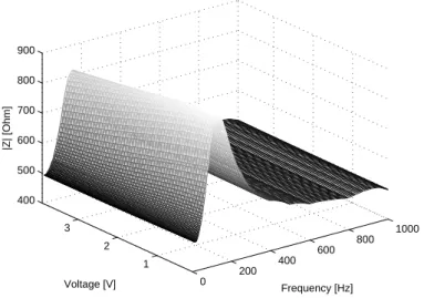
0 200 400 600 800 1000 1 2 3 400 500 600 700 800 900 Frequency [Hz] Voltage [V] |Z| [Ohm]
Fig. 1. Experimental three-dimensional representation of the electrical impedance magnitude of the electrodynamic microphone (voltage: 0 V;4 V)(frequency: 0 Hz;1000 Hz)(|Z|: 400Ω;900Ω)
2.1 Limits of a linear electro-acoustical model
118
This section presents the limits of the linear model for characterizing
elec-119
trodynamic microphones. To do so, an electrodynamic microphone is placed
120
in an anechoic chamber. An electrical impedance measurement is realized by
121
using a Wayne Kerr wedge that has an excellent precision (10−4Ω). A voltage 122
measurement is carried out with levels varying from 100mV to 4V. During our
123
experiment, the electrodynamic microphone is used as an acoustical source.
124
Even though this situation is rather rare, the nonlinearities determined with
125
such an approach represent very well the main defects in electrodynamic
mi-126
crophones. This is in fact the main aim of this paper: an accurate electrical
127
impedance measurement can be used to estimate electrodynamic microphone
128
nonlinearities. The electrical impedance magnitude is represented versus the
129
input voltage and the frequency in Fig.(1) while its phase is represented in
130
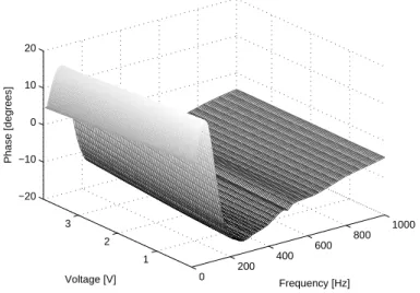
Fig. (2) A two-dimensional view allows us to see more precisely the
0 200 400 600 800 1000 1 2 3 −20 −10 0 10 20 Frequency [Hz] Voltage [V] Phase [degrees]
Fig. 2. Experimental three-dimensional representation of the electrical impedance phase of the electrodynamic microphone (voltage: 0 V;4 V)(frequency: 0 Hz;1000 Hz)(phase: -20 deg ;+20 deg)
100 120 140 160 180 200 220 240 260 700 750 800 850 900 Frequency [Hz] |Z| [Ohm] 0.1V 0.9V 1.9V 2.9V 3.9V
Fig. 3. Two-dimensional representation of the electrical impedance magnitude of the electrodynamic microphone (frequency: 100 Hz;260 Hz)(|Z|: 700 Ω; 900 Ω)
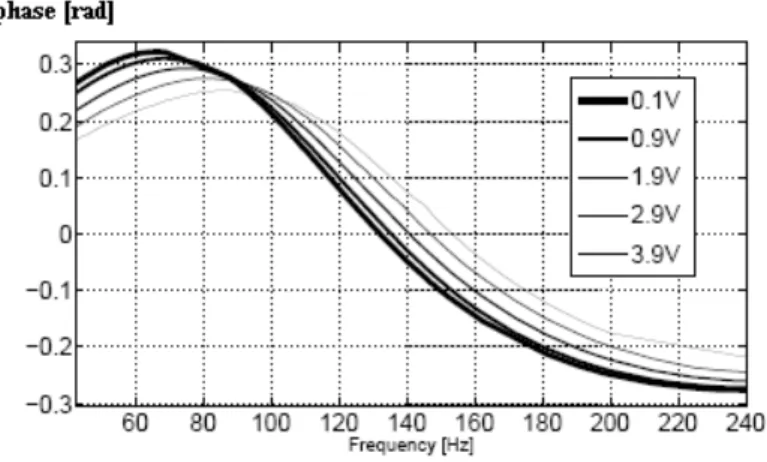
ear phenomena of the two previous representations (Figs. 3 and 4). Figures
132
3 and 4 shows that the electrical impedance of the electrodynamic
micro-133
phone depends also on input voltage. It is noted that the resonance frequency
134
varies with respect to the input voltage; this implies that the stiffness of the
135
suspensions or the equivalent mass depend on input voltage. In conclusion,
136
Eq.(4) which is generally used to describe the electrodynamic microphone is
137
not sufficient to correctly describe its nonlinear effects. Strictly speaking, all
Fig. 4. Two-dimensional representation of the electrical impedance phase of the electrodynamic microphone (frequency: 60 Hz;240 Hz)(phase: -0.3 rad;+0.3 rad)
the parameters which define the electrical impedance (Eq.4) are a function of
139
both input level and time. Obtaining the variation laws of these parameters
140
is necessary in order to improve the design of electrodynamic microphones
141
and predict the distortions created by themselves. As a consequence, a
gen-142
eral method should be found in order to determine which parameters vary
143
a lot with the input voltage and produce some distortions. Such a general
144
experimental method is discussed in the next section.
145
3 Experimental method to derive the nonlinear variations of the
146
Thiele and Small parameters
147
3.1 Introduction
148
Our experimental method to derive the dependence of the Thiele and Small
149
parameters with the input voltage is based on the electrical impedance
mea-150
surement of the electrodynamic microphone. A real-time algorithm has been
151
put forward to measure this impedance with a Wayne Kerr wedge that has an
excellent precision (10−4Ω). It is noted that this wedge is especially dedicated 153
to the electrical impedance measurement. Consequently, we can say that such
154
a measurement device allows us to have a great confidence in the experimental
155
measurements. Our way of characterizing the electrodynamic microphone
non-156
linearities allows us to predict precisely the distortions created by such
trans-157
ducers. Our measurement algorithm is used in order to determine at which
158
frequencies impedance must be measured. Basically, points must be measured
159
when electrical impedance reaches a maximum or when impedance variation
160
with frequency is important. In short, the electrodynamic microphone is
char-161
acterized by its electrical impedance which, precisely measured, allows us to
162
construct polynomial functions for each electrodynamic microphone
parame-163
ter. The polynomial functions are determined by using Simplex algorithm and
164
their coefficients are established by using the least mean square method. The
165
Simplex algorithm is used to determine the coefficients of each polynomial
166
function describing the nonlinear variations of the Thiele and Small
parame-167
ters. The principle of this algorithm is to minimize the difference ∆Ze between 168
the experimental impedance and the theoretical impedance. The theoretical
169
impedance is in fact the electrical impedance with the Thiele and Small model
170
whose parameters are assumed to depend on input voltage. For example, the
171
equivalent mass can be written :
172 Mms(u) = Mms+ m X n=1 ˜ µnM msun (5) 173
Each Thiele and Small parameter is represented like the previous form.
Con-174
sequently, the difference ∆Ze is expressed as follows: 175 ∆Z = n=2 X n=0 ¯ ¯ ¯ ¯ ¯ ¯Z
(exp)(u) − Z(theo)(u)¯ ¯ ¯ ¯ ¯ ¯ 2 (6) 176
where
177 178
Z(theo)(u) = Re(u) +
jRµ(u)Le(u)w
jLe(u)w + Rµ(u)
+ Bl(u)
2
Rms(u) + jMms(u)w + jCms(u)w1
(7) When the algorithm converges, all the values describing the nonlinear
param-179
eters obtained are used to solve numerically the nonlinear differential equation
180
of the electrodynamic microphone. Figure 5 represents the error sheet between
181
the experimental results and the theoretical ones when the Thiele and Small
182
parameters are constant. The mean difference between the experimental and
183
the theoretical values is 6.0Ω. In this case, we did not take into account the
184
nonlinear variations of the Thiele and Small parameters determined by the
185
Simplex algorithm. Figure (6) represents the error sheet between the
experi-186
mental resuts and the theoretical one when the variations of the Thiele and
187
Small parameters are taken into account. The mean difference between the
ex-188
perimental and the theoretical values is 2.9Ω. As a consequence, the
improve-189
ment of the electrodynamic microphone model is only possible if the nonlinear
190
variations of the Thiele and Small parameters are taken into account.
191
3.2 Variations of the Thiele and Small parameters
192
This section discusses the sensitivity of the Thiele and Small parameters to
193
the least mean square method. To do so, we assume that only one parameter
194
varies at a time (though the other Thiele and Small parameters are constant).
195
By using our least square method based on the simplex method, we determine
196
the difference of the impedance (magnitude and phase) between the model
197
with constant parameters and the model with one varying parameter. This
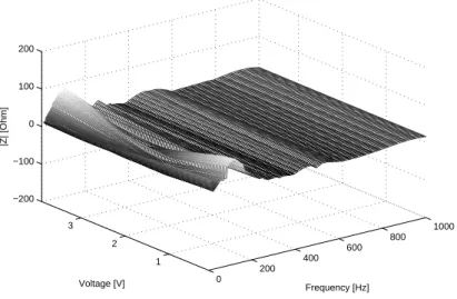
0 200 400 600 800 1000 1 2 3 −200 −100 0 100 200 Frequency [Hz] Voltage [V] |Z| [Ohm]
Fig. 5. Three-dimensional representation of the difference between the experimental impedance and the theoretical impedance ; the theoretical impedance is based on the Thiele and Small model with constant parameters (voltage: 0 V;4 V)(frequency: 0 Hz;1000 Hz)(|Z|: -200Ω;+200Ω) 0 200 400 600 800 1000 1 2 3 −200 −100 0 100 200 Frequency [Hz] Voltage [V] |Z| [Ohm]
Fig. 6. Three-dimensional representation of the difference between the experimental impedance and the theoretical impedance ; the theoretical impedance is based on the Thiele and Small model with variable parameters (voltage: 0 V;4 V)(frequency: 0 Hz;1000 Hz)(|Z|: -200Ω;+200Ω)
Parameter Law of variation sensitivity Re 490.1 Le 0.0023 + 0.002u + 0.06u2 15.1% Bl 13.2 − 15.1u + 8.09u2 23% Rms 0.25 + 0.81u − 0.021u2 4.7% M ms 0.00025 − 0.0014u + 0.0036u2 18.1% k 171.28 − 50.2u + 1018u2 2.1% Rµ 48.1 Table 1
Laws of variations of the Thiele and Small parameters
difference allows us to determine the sensitivity of each Thiele and Small
pa-199
rameter. Table 1 presents the laws of variations of Thiele and Small parameters
200
determined with our three-dimensional least mean square method.
201
It can be noted that the parameter that is the most sensitive to the least mean
202
square algorithm is the force factor Bl. In addition, we see that the equivalent
203
inductance Leis also sensitive. This implies that the magnetic circuit could be 204
improved. In fact, it is well-known that the iron in magnetic circuits generates
205
nonlinearities because of its saturation and its hysteresis losses. This is the
206
reason why it can be interesting to design ironless magnetic loudspeakers [20].
3.3 Obtaining the nonlinear differential equation of the electrodynamic
mi-208
crophone
209
This section presents a method to obtain the nonlinear differential equation
210
of the electrodynamic microphone. In fact, this nonlinear differential
equa-211
tion is the same as the one of the electrodynamic loudspeaker because the
212
electrodynamic microphone is used as an acoustical source. In this paper, the
213
nonlinear differential equation of the electrodynamic microphone is obtained
214
by taking into account the variations of the Thiele and Small parameters.
215
These variations are obtained in the previous section by using both the
Sim-216
plex algorithm with the least mean square criteria. Furthermore, we neglect
217
here the unstationary effects (Re increases in time due to the Joule effect). 218
The first step for obtaining this nonlinear differential equation is to drop the
219
parameter i(t) from the two equations (1) and (2). From (2), i(t) can also be
220 written as follows: 221 i(t) = 1 Bl à Mms d2x(t) dt2 + Rms dx(t) dt + kx(t) ! (8) 222
By using (8) and 1, we deduct :
223 224 u(t) =Re Bl à Mms d2x(t) dt2 + Rms dx(t) dt + kx(t) ! +Bldx(t) dt + Le Bl à Mms d3x(t) dt3 + Rms d2x(t) dt2 + k dx(t) dt ! (9) The previous equation can also be written in the following form :
225 u(t) = ad 3x(t) dt3 + b d2x(t) dt2 + c dx(t) dt + dx(t) (10) 226
with 227 a= MmsLe Bl (11) 228 b= (MmsRe+ RmsLe) Bl (12) 229 c= (ReRms+ Bl 2+ kL e) Bl (13) 230 d= kRe Bl (14) 231
We can also write the previous relations in the frequency domain so that (10)
232
becomes :
233
U = a(jw)3X+ b(jw)2X+ c(jw)X + dX (15)
234
Thus, we deduct that there is a bijective relation between U and X:
235 U = X³A(jw)3 + B(jw)2+ C(jw) + D´ (16) 236 Thus 237 U = χX (17) 238
where χ = (A(jw)3+ B(jw)2+ C(jw) + D). In the previous section, we
stud-239
ied the fact that the five Small signal parameters depended on input voltage.
240
We deduct that these parameters can also be written as a function of the
241
voice coil position X. Therefore, the parameters a, b, c and d in 10 become
242
a(x), b(x), c(x) and d(x) in the nonlinear differential equation of the
electro-243
dynamic microphone. It is to be noted that solving this nonlinear differential
244
equation is rather difficult because the denominator is not constant. It can
be noted that this equation must be solved numerically in order to determine
246
the distortions created by an electrodynamic microphone. In fact, the
distor-247
tions created by a nonlinear system can be determined either analytically by
248
using for example a Taylor series expansion or numerically. In the case of the
249
electrodynamic microphone, we have chosen to solve numerically its nonlinear
250
differential equation with Mathematica. This allows us to confirm the
experi-251
mental displacement spectrum measured with the laser Doppler velocimeter.
252
3.4 Comparison between the theoretical displacement spectrum and the
ex-253
perimental displacement spectrum
254
A way of obtaining the theoretical displacement spectrum is to solve
numer-255
ically the nonlinear differential equation of the electrodynamic microphone.
256
This can be done for example in the time-domain by assuming that the
elec-257
trodynamic microphone generates only harmonics that are multiple of the
258
fundamental harmonic (w, 2w, 3w ). This is a simplifying assumption because
259
input voltage owns in reality many terms so that other typical nonlinear
phe-260
nomena appear (intermodulations). In short, we assume the solution of the
261
nonlinear differential equation of the electrodynamic microphone to be as the
262
following form:
263
x(t) = a1cos(wt) + a2sin(wt) + a3cos(2wt) + a4sin(2wt)
+a5cos(3wt) + a6sin(3wt)
(18)
The parameters a1, a2, a3, a4, a5 and a6 are determined numerically and are 264
given in Table 2.
Coefficient Value a1 5.210−3 a2 0.8310−3 a3 2.4510−12 a4 4.1810−13 a5 8.8310−16 a6 6.1210−16 Table 2
Values of the coefficients given in Eq. (18) : these coefficients have been determined with the explicit Runge Kutta method (numerical solving of the nonlinear differen-tial equation of the electrodynamic microphone)
3.5 Experimental and theoretical displacement spectrums
266
This section presents a comparison between the experimental displacement
267
spectrum of the electrodynamic microphone which has been obtained by
us-268
ing a laser Doppler velocimeter and the theoretical displacement spectrum
269
obtained by using the solution given in Eq. (18). The experimental and
theo-270
retical values are given in table 3. Moreover, the results obtained are plotted
271
in Fig. 7. The theoretical displacement spectrum is consistent with the
ex-272
perimental displacement spectrum. Consequently, we deduct that the
experi-273
mental way of characterizing the electrodynamic microphone with its electrical
274
impedance allows us to precisely estimate the nonlinear variations of the Small
275
signal parameters with the input voltage.
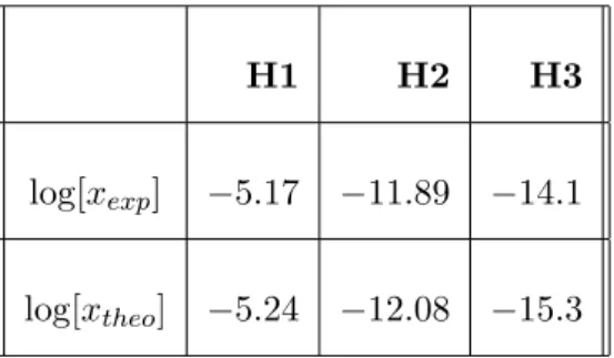
H1 H2 H3
log[xexp] −5.17 −11.89 −14.1
log[xtheo] −5.24 −12.08 −15.3
Table 3
Values of the harmonics created by the electrodynamic microphone ; H1 corresponds to the fundamental, H2 is the harmonic two and H3 is the harmonic three
Fig. 7. Experimental and Theoretical spectrums of the electrodynamic microphone
4 Conclusion
277
In this paper, we studied the nonlinear effects of electrodynamic microphones
278
that occur when they are used as acoustical sources. This functioning occurs
279
in reciprocal calibration techniques. An experimental method, based on a very
280
precise electrical impedance measurement allows us to put forward a
measure-281
ment algorithm which is used to acquire as many points as possible. This
mea-282
surement algorithm has been put forward in the case of the nonlinear study of
283
electrodynamic loudspeakers. Taking into account the variations of the Small
284
signal parameters with the input voltage allows us to improve significantly the
285
model of the electrodynamic microphone. The variations of the Small signal
286
parameters generate any distortions. These distortions can be predicted by
solving numerically the nonlinear differential equation of the electrodynamic
288
microphone. The comparison between the theoretical displacement spectrum
289
and the experimental displacement spectrum shows a very good agreement at
290
low frequencies.
291
References
[1] M. T. Abuelma’atti, “Improved analysis of the electrically manisfested distortions of condenser microphones,” Applied Acoustics, vol. 64, pp. 471–480, May 2003.
[2] M. T. Abuelma’atti, “Harmonic and intermodulation distortion in electret microphones,” Applied Acoustics, vol. 34, no. 1, pp. 1–6, 1991.
[3] M. T. Abuelma’atti, “Large signal performance of micromachinened silicon condenser microphones,” Applied Acoustics, vol. 68, pp. 1286–1296, October 2007.
[4] M. Niewiarowicz, “Investigations into the transduction properties of dynamic microphone membranes subjected to transients,” Applied Acoustics, vol. 22, no. 3, pp. 177–183, 1987.
[5] M. Niewiarowicz, “Determination of active compliance of dome type microphone membranes by using the indicator diagrams method,” Journal of Sound and
Vibration, vol. 182, no. 4, pp. 589–594, 1995.
[6] S.-M. Hwang, H.-J. Lee, K.-S. Hong, B.-S. Kang, and G.-Y. Hwang, “New develpment of combined permanent-magnet type microspeakers used for cellular phones,” IEEE Trans. Magn, vol. 41, no. 5, pp. 2000–2003, 2005.
[7] P. C. P. Chao, C. W. Chiu, and Y. Hsu-Pang, “Magneto-electrodynamical modeling and design of a microspeaker used for mobile phones with
considerations of diaphragm corrugation and air closures,” IEEE Trans. Magn, vol. 43, no. 6, pp. 2585–2587, 2007.
[8] P. C. P. Chao and S.-C. Wu, “Optimal design of magnetic zooming mechanism used in cameras of mobile phones via genetic algorithm,” IEEE Trans. Magn, vol. 43, no. 6, pp. 2579–2581, 2007.
[9] E. Sadikog, “A laser pistonphone based on self-mixing interferometry for the absolute calibration of measurement microphones,” Applied Acoustics, vol. 65, no. 9, pp. 833–840, 2004.
[10] T. Musha and J. I. Taniguchi, “Measurement of sound intensity using a single moving microphone,” Applied Acoustics, vol. 66, no. 5, pp. 579–589, 2005.
[11] E. R. Olsen and K. B. Christensen, “Nonlinear modeling of low frequency loudspeakers- a more complete model,” in 100th convention, Copenhagen, no. 4205, Audio Eng. Soc., 1996.
[12] J. W. Noris, “Nonlinear dynamical behavior of a moving voice coil,” in 105th
convention, San Francisco, no. 4785, Audio Eng. Soc., 1998.
[13] A. Dobrucki, “Nontypical effects in an electrodynamic loudspeaker with a nonhomogeneous magnetic field in the air gap and nonlinear suspension,” J.
Audio Eng. Soc., vol. 42, pp. 565–576, 1994.
[14] M. R. Gander, “Dynamic linearity and power compression in moving-coil loudspeaker,” J. Audio Eng. Soc., pp. 627–646, September 1986.
[15] M. R. Gander, “Moving-coil loudspeaker topology as an indicator of linear excursion capability,” J. Audio Eng. Soc., vol. 29, 1981.
[16] W. M. Leach, “Loudspeaker voice-coil inductance losses : Circuit models, parameter estimation and effect on frequency response,” J. Audio Eng. Soc., pp. 442–449, 2002.
[17] J. R. Wright, “An empirical model for loudspeaker motor impedance,” J. Audio
Eng. Soc., pp. 749–754, October 1990.
[18] W. Klippel, “Loudspeaker nonlinearities - cause, parameters, symptoms,” J.
Audio Eng. Soc., vol. 54, pp. 907–939, 2006.
[19] R. Ravaud, G. Lemarquand, V. Lemarquand, and C. Depollier, “Ironless loudspeakers with ferrofluid seals,” Archives of Acoustics, vol. 33, no. 4, pp. 3– 10, 2008.
[20] G. Lemarquand, “Ironless loudspeakers,” IEEE Trans. Magn., vol. 43, no. 8, pp. 3371–3374, 2007.
[21] R. H. Small, “Closed-box loudspeaker systems, part1: Analysis,” J. Audio Eng.
Soc., vol. 20, no. 12, pp. 798–808, 1972.
[22] R. Ravaud, G. Lemarquand, and T. Roussel, “Time-varying nonlinear modeling of electrodynamic loudspeakers,” Applied Acoustics, vol. 70, no. 3, pp. 450–458, 2009.
[23] A. N. Thiele, “Loudspeakers in vented boxes, part i,” J Audio Eng Soc, vol. 19, pp. 382–392, 1971.
[24] A. N. Thiele, “Loudspeakers in vented boxes, part ii,” J Audio Eng Soc, vol. 19, pp. 471–483, 1971.
[25] R. H. Small, “Direct-radiator loudspeaker system analysis,” J. Audio Eng. Soc., vol. 20, no. 6, pp. 383–395, 1972.
[26] J. Vanderkooy, “A model of loudspeaker driver impedance incorporating eddy currents in the pole structure,” J. Audio Eng. Soc., vol. 37, pp. 119–128, March 1989.