HAL Id: hal-01587520
https://hal.archives-ouvertes.fr/hal-01587520
Submitted on 3 May 2021
HAL is a multi-disciplinary open access
archive for the deposit and dissemination of
sci-entific research documents, whether they are
pub-lished or not. The documents may come from
teaching and research institutions in France or
abroad, or from public or private research centers.
L’archive ouverte pluridisciplinaire HAL, est
destinée au dépôt et à la diffusion de documents
scientifiques de niveau recherche, publiés ou non,
émanant des établissements d’enseignement et de
recherche français ou étrangers, des laboratoires
publics ou privés.
Intercomparison Project: experimental protocol for
CMIP6
Chris D. Jones, Vivek Arora, Pierre Friedlingstein, Laurent Bopp, Victor
Brovkin, John John, Heather Graven, Forrest Hoffman, Tatiana Ilyina, Jasmin
G. John, et al.
To cite this version:
Chris D. Jones, Vivek Arora, Pierre Friedlingstein, Laurent Bopp, Victor Brovkin, et al.. C4MIP
– The Coupled Climate–Carbon Cycle Model Intercomparison Project: experimental protocol for
CMIP6. Geoscientific Model Development, European Geosciences Union, 2016, 9 (8), pp.2853 - 2880.
�10.5194/gmd-9-2853-2016�. �hal-01587520�
www.geosci-model-dev.net/9/2853/2016/ doi:10.5194/gmd-9-2853-2016
© Author(s) 2016. CC Attribution 3.0 License.
C4MIP – The Coupled Climate–Carbon Cycle Model
Intercomparison Project: experimental protocol for CMIP6
Chris D. Jones1, Vivek Arora2, Pierre Friedlingstein3, Laurent Bopp4, Victor Brovkin5, John Dunne6, Heather Graven7, Forrest Hoffman8, Tatiana Ilyina5, Jasmin G. John6, Martin Jung9, Michio Kawamiya10, Charlie Koven11, Julia Pongratz5, Thomas Raddatz5, James T. Randerson12, and Sönke Zaehle9
1Met Office Hadley Centre, Exeter, EX1 3PB, UK
2Canadian Centre for Climate Modelling and Analysis, Climate Research Division, Environment and Climate Change,
Victoria, Canada
3College of Engineering, Mathematics and Physical Sciences, University of Exeter, Exeter, EX4 4QE, UK
4Laboratoire des Sciences du Climat et de l’Environnement, LSCE/IPSL, CEA-CNRS-UVSQ, Université Paris-Saclay, 91191
Gif-sur-Yvette, France
5Max Planck Institute for Meteorology, Hamburg, Germany 6NOAA/GFDL, Princeton, NJ, USA
7Department of Physics and Grantham Institute, Imperial College London, London, UK 8Oak Ridge National Lab., Oak Ridge, TN, USA
9Biogeochemical Integration Department, Max Planck Institute for Biogeochemistry, 07745 Jena, Germany 10Japan Agency for Marine-Earth Science and Technology, Kanagawa, Japan
11Earth Sciences Division, Lawrence Berkeley National Laboratory, Berkeley, CA, USA 12Department of Earth System Science, University of California, Irvine, CA USA
Correspondence to:Chris D. Jones ([email protected])
Received: 12 February 2016 – Published in Geosci. Model Dev. Discuss.: 16 March 2016 Revised: 1 July 2016 – Accepted: 5 July 2016 – Published: 25 August 2016
Abstract. Coordinated experimental design and implemen-tation has become a cornerstone of global climate modelling. Model Intercomparison Projects (MIPs) enable systematic and robust analysis of results across many models, by reduc-ing the influence of ad hoc differences in model set-up or ex-perimental boundary conditions. As it enters its 6th phase, the Coupled Model Intercomparison Project (CMIP6) has grown significantly in scope with the design and documenta-tion of individual simuladocumenta-tions delegated to individual climate science communities.
The Coupled Climate–Carbon Cycle Model Intercompar-ison Project (C4MIP) takes responsibility for design, docu-mentation, and analysis of carbon cycle feedbacks and in-teractions in climate simulations. These feedbacks are poten-tially large and play a leading-order contribution in determin-ing the atmospheric composition in response to human emis-sions of CO2and in the setting of emissions targets to
sta-bilize climate or avoid dangerous climate change. For over
a decade, C4MIP has coordinated coupled climate–carbon cycle simulations, and in this paper we describe the C4MIP simulations that will be formally part of CMIP6. While the climate–carbon cycle community has created this experimen-tal design, the simulations also fit within the wider CMIP ac-tivity, conform to some common standards including docu-mentation and diagnostic requests, and are designed to com-plement the CMIP core experiments known as the Diagnos-tic, Evaluation and Characterization of Klima (DECK).
C4MIP has three key strands of scientific motivation and the requested simulations are designed to satisfy their needs: (1) pre-industrial and historical simulations (formally part of the common set of CMIP6 experiments) to enable model evaluation, (2) idealized coupled and partially coupled sim-ulations with 1 % per year increases in CO2 to enable
di-agnosis of feedback strength and its components, (3) future scenario simulations to project how the Earth system will
re-spond to anthropogenic activity over the 21st century and be-yond.
This paper documents in detail these simulations, explains their rationale and planned analysis, and describes how to set up and run the simulations. Particular attention is paid to boundary conditions, input data, and requested output diag-nostics. It is important that modelling groups participating in C4MIP adhere as closely as possible to this experimental design.
1 Introduction
Over the industrial era since about 1750, it is estimated that cumulative anthropogenic carbon emissions from fos-sil fuels and cement (405 ± 20 PgC) and land-use change (190 ± 65 PgC) have been partitioned between the atmo-sphere (255 ± 5 PgC), the ocean (170 ± 20 PgC), and the terrestrial biosphere (165 ± 70 PgC) (values to the nearest 5 PgC, from Le Quéré et al., 2015). The carbon uptake by land and ocean, since the start of the industrial era, has thus slowed the rate of increase of atmospheric CO2concentration
in response to anthropogenic carbon emissions. Had the land and ocean not provided this “ecosystem service”, the atmo-spheric CO2concentration at present would be much higher.
The manner in which the land and ocean will continue to absorb anthropogenic carbon emissions has both scientific and policy relevance. Understanding the future partitioning of anthropogenic CO2 emissions into the atmosphere, land
and ocean components, and the resulting climate change, ac-counting for biogeochemical feedbacks requires a full Earth system approach to modelling the climate and carbon cycle.
The primary focus of the Coupled Climate–Carbon Cy-cle Model Intercomparison Project (C4MIP; http://www. c4mip.net) is to understand and quantify future century-scale changes in land and ocean carbon storage and fluxes and their impact on climate projections. In order to achieve this, a set of Earth system model (ESM) simulations has been devised. As a consequence of the very high computational demand on modelling centres to perform a multitude of simulations for many different intercomparison studies as part of CMIP6, we have carefully chosen a minimum set of targeted simulations to achieve C4MIP goals. They comprise
– idealized experiments, which will be used to separate and quantify the sensitivity of land and ocean carbon cycle to changes in climate and atmospheric CO2
con-centration;
– historical experiments, which will be used to evaluate model performance and investigate the potential for us-ing contemporary observations as a constraint on future projections;
– future scenario experiments, which will be used to quantify future changes in carbon storage and hence
quantify the atmospheric CO2concentration and related
climate change for a given set of CO2 emissions, or,
conversely, to diagnose the emissions compatible with a prescribed atmospheric CO2concentration pathway.
The simulations are designed to complement those requested in the CMIP6 Diagnostic, Evaluation and Characterization of Klima (DECK) and the CMIP6 historical simulation (Eyring et al., 2016a). They also align closely with simulations per-formed as part of ScenarioMIP (O’Neill et al., 2016) by quantifying the role of carbon cycle feedbacks in the evolu-tion of atmospheric CO2due to anthropogenic carbon
emis-sions. Synergies with other MIPs are discussed in Sect. 2. C4MIP simulations and analyses will play a major role contributing to the WCRP Carbon Feedbacks in the Cli-mate System – Grand Challenge (http://www.wcrp-cliCli-mate. org/gc-carbon-feedbacks). This is the third generation of C4MIP following the first coordinated experiments described in Friedlingstein et al. (2006) and the carbon cycle simula-tions that formed part of CMIP5 (Taylor et al., 2012).
In this paper we first briefly describe the scientific ra-tionale and motivation for the C4MIP simulations and then carefully document the experimental protocol in Sect. 3. Modelling groups intending to participate in C4MIP should follow the design described here as closely as possible. Par-ticular attention should be given to the set-up of bound-ary conditions in terms of atmospheric CO2 concentration
or emissions and which aspects of the model experience changes in the fully coupled or partially coupled simulations. Output requirements (diagnostics) are also carefully docu-mented in Sect. 4.
Along with our science motivation (Sect. 2), we highlight initial plans for the analyses of the carbon cycle and its inter-actions with the physical climate system. Modelling groups will be invited to contribute to the primary C4MIP analysis papers. We anticipate, and hope, that many further studies and analyses will also be conducted throughout the climate– carbon cycle research community and that these simulations provide a valuable resource to further carbon cycle research.
2 Background and science motivation 2.1 C4MIP history
The potential for a climate feedback on the carbon cycle whereby carbon released due to warming would further el-evate atmospheric CO2 and amplify climate change was
first discussed in the late 1980s–early 1990s (e.g. Lashof et al., 1989; Jenkinson et al., 1991; Schimel et al., 1994; Kirschbaum, 1995; Sarmiento and Le Quéré, 1996). On the land side, dynamic global vegetation models were used to study the impact of rising CO2 and climate change on the
carbon cycle (Cramer et al., 2001). There was a strong model consensus that rising CO2 would stimulate additional
likewise warming climate would accelerate decomposition of dead organic matter and may also reduce vegetation produc-tivity in some (mainly tropical) ecosystems (Prentice et al., 2001). Similarly for the ocean, there was also a model con-sensus that warming would lead to reduced carbon uptake (Prentice et al., 2001). This was due to both reduced solu-bility in warmer waters and reduced rate of transport of an-thropogenic carbon to the deep ocean as a consequence of in-creasing stratification and shutdown of meridional overturn-ing circulation. The processes behind the former (carbonate chemistry and solubility) were reasonably well understood (Bacastow, 1993), but the latter was much more uncertain being sensitive to the underlying ocean model circulation (Maier-Reimer et al., 1996; Sarmiento et al., 1998; Joos et al., 1999). The role of ocean biology and the buffering ca-pacity of the ocean were also seen to be important and not well constrained or represented in models (Sarmiento and Le Quéré, 1996).
These “offline” land and ocean experiments found poten-tially high sensitivity of the carbon cycle to environmental forcing but were not able to simulate the full effect of this feedback onto climate. By the end of the 1990s some mod-elling groups were beginning to implement interactive car-bon cycle modules in their physical climate models. These early studies (e.g. Cox et al., 2000; Friedlingstein et al., 2001; Dufresne et al., 2002; Thompson et al., 2004) were able to recreate an experimental setting more like the real world where a climate change forced by anthropogenic CO2
emis-sions would affect natural carbon sinks and stores, which in turn would affect changes in atmospheric CO2and hence
cli-mate.
It soon became apparent from the first publications that there were substantial differences in the sensitivities of these new models. The desire to understand and reduce this un-certainty led to the development of a linearized feedback framework to diagnose the sensitivity of different parts of the system and their contribution to the overall feedback (Friedlingstein et al., 2003), and also of a multi-model inter-comparison activity (C4MIP: Coupled Climate–Carbon Cy-cle Model Intercomparison; Fung et al., 2000). The result was the first C4MIP intercomparison paper, (Friedlingstein et al., 2006), which quantified the feedback components across 11 models for a common CO2emissions scenario. All
mod-els agreed qualitatively that the sign of the carbon–climate feedback was positive – i.e. the interaction of the carbon cy-cle with climate led to reduced carbon uptake and hence an increase in atmospheric CO2, which amplified the initial
cli-mate change. However, there was large quantitative model spread in the total feedback and its sensitivity components. Initial analysis of the causes of this uncertainty concluded that the land played a greater role than the ocean, in partic-ular its sensitivity to climate. Regionally, the tropics were seen to be particularly different between models (Raddatz et al., 2007), bearing in mind that none of these models in-cluded representation of permafrost carbon. The CMIP5
ex-perimental design for carbon cycle feedback diagnosis (Tay-lor et al., 2012) closely followed the C4MIP protocol. Mod-elling centres around the world contributed results to CMIP5 and their analysis led to many key papers including a special collection of 15 papers published in the Journal of Climate (http://journals.ametsoc.org/topic/c4mip).
The C4MIP activity under CMIP5 was central to Working Group 1 of the IPCC 5th Assessment. Several of the main findings from C4MIP studies were included in the Summary for Policymakers of WG1, such as the positive feedback be-tween climate and carbon cycle – “climate change will af-fect carbon cycle processes in a way that will exacerbate the increase of CO2 in the atmosphere”; the impact of elevated
CO2 on ocean acidification – “further uptake of carbon by
the ocean will increase ocean acidification”; the emissions compatible with given CO2concentrations – “by the end of
the 21st century, [for RCP2.6] about half of the models in-fer emissions slightly above zero, while the other half inin-fer a net removal of CO2 from the atmosphere”; and the very
policy relevant relationship between cumulative CO2
emis-sions and global warming – “cumulative emisemis-sions of CO2
largely determine global mean surface warming by the late 21st century and beyond”.
2.2 Key science motivation and analysis plans for C4MIP
The key science motivations behind C4MIP are (1) to quan-tify and understand the carbon-concentration and carbon– climate feedback parameters which respectively, capture the modelled response of land and ocean carbon cycle compo-nents to changes in atmospheric CO2and the associated
cli-mate change; (2) to evaluate models by comparing histori-cal simulations with observation-based estimates of climato-logical states of carbon cycle variables, their variability, and long-term trends; (3) to assess the future projections of the components of the global carbon budget for different scenar-ios, including atmospheric CO2concentration, atmosphere–
land and atmosphere–ocean fluxes of CO2, diagnosed CO2
emissions compatible with future scenarios of CO2
path-way and crucially to provide new estimates of the cumu-lative CO2 emissions compatible with specific climate
tar-gets. In light of the COP21 Paris agreement (https://unfccc. int/resource/docs/2015/cop21/eng/l09r01.pdf), these experi-ments will quantify carbon cycle feedbacks in low emissions scenarios and inform cumulative budgets consistent with a 1.5 or 2◦C stabilization objective.
Relative to CMIP5 there are three key areas where we ex-pect CMIP6 models to have made substantial progress and hence may cause significant differences in the simulated re-sponse of the carbon cycle to anthropogenic forcing.
i. In CMIP5, only two participating ESMs included a land surface component (CLM4) that explicitly considered constraints of terrestrial N availability on primary pro-duction and net land carbon storage (Lindsay et al.,
2014; Tjiputra et al., 2013). An increasing number of land models now include a prognostic representation of the terrestrial N cycle and its coupling to the land C cy-cle (Zaehle and Dalmonech, 2011). Some of these prog-nostic N cycle representations are expected to be used in land components of ESMs participating in CMIP6. Coupling of carbon and nitrogen dynamics changes the response of the terrestrial biosphere to global change in four ways: (1) it generally reduces the response of net primary production and carbon storage to elevated lev-els of atmospheric CO2because of an increasing limit of
nitrogen availability for carboxylation enzymes and new tissue construction; (2) it allows for changes in plant al-location in response to changing nutrient availability; (3) it generally decreases net ecosystem C losses as-sociated with soil warming, because increased decom-position leads to increased plant N availability, which can potentially increase plant productivity and C stor-age in N-limited ecosystems; and (4) it alters primary production due to anthropogenic N deposition and fer-tilizer application, which may regionally enhance net C uptake. The magnitude of each of these processes is un-certain given strong natural gradients in the natural N availability in ecosystems and sparse ecosystem data to constrain these models (Thornton et al., 2009; Zaehle et al., 2014; Meyerholt and Zaehle, 2015) but offline anal-ysis of CMIP5 simulations suggests significant overes-timation of terrestrial carbon uptake in models that ne-glect the role of nitrogen (Wieder et al., 2015; Zaehle et al., 2015). The new generation of models will provide a more comprehensive assessment of the attenuating ef-fect of nitrogen on carbon cycle dynamics compared to CMIP5 and in particular provide a better constrained estimate of the carbon storage capacity of land ecosys-tems.
ii. In CMIP5, all land models used a single-layer, verti-cally integrated representation of soil biogeochemistry (Luo et al., 2016). Such an approach necessarily ignores vertical variation in soil carbon turnover times, which can be very important in governing ecosystem carbon storage. This omission is most notable in the extreme case of permafrost soils, where there exists a depth at which soils remain frozen year-round and, because of the abrupt change in decomposition rates in frozen vs. unfrozen soils, otherwise highly decomposable carbon can be preserved indefinitely until it is thawed. The majority of global soil carbon is in permafrost-affected ecosystems, which creates the possibility for permafrost climate feedbacks (Burke et al., 2013). Some of the models in CMIP6 are expected to include representa-tion of permafrost soil carbon dynamics, either explic-itly by representing soil biogeochemistry along the full soil depth axis (Koven et al., 2013), or by means of reduced-complexity methods to incorporate permafrost
dynamics. IPCC Fifth Assessment Report (AR5) con-cluded that permafrost carbon release was likely, and therefore would increase the climate–carbon cycle feed-back, but with low confidence in the magnitude (Ciais et al., 2013). Assessing the role of this process in govern-ing fully coupled climate feedbacks will be an important contribution to CMIP6.
iii. Representation of ocean dynamics in the ESMs is an-other important constraint affecting the oceanic carbon uptake and storage. There is evidence that by shifting to an eddy-permitting grid configuration of the ocean general circulation model, the representation of some key features of oceanic circulation, such as the interior water-mass properties and surface ocean current sys-tems, are improved (Jungclaus et al., 2013). The in-creased horizontal resolution of the underlying ocean model has a positive impact on the performance of the marine biogeochemistry model in the deeper layers (Ily-ina et al., 2013). Spatial resolution of some ESMs is expected to increase as they move into CMIP6. The increased resolution of the oceanic components of the ESMs is expected to have some explicit advantages for projections of the oceanic carbon uptake. First, it al-lows us to estimate the role of previously unresolved small-scale ocean hydrodynamical process on projec-tions of marine biogeochemistry. Second, by improving the representation of coastal processes and ocean–shelf exchange, their contribution to the global carbon cycle can be assessed.
2.2.1 Carbon cycle feedback parameters
The first key motivation for C4MIP is to document the changes in magnitude of the feedback parameters that char-acterize the response of the carbon cycle and their spread across models through time. In this respect, C4MIP aims to calculate the magnitude of the carbon-concentration and carbon–climate feedbacks in a manner similar to Friedling-stein et al. (2006) or Arora et al. (2013) and as discussed in Sect. 3.1 using results from the idealized 1 % per year in-creasing CO2experiments.
The 1pctCO2 experiment has gained recognition as a stan-dard CMIP simulation and it is one of the DECK simulations for CMIP6 (Eyring et al., 2016a). The 1pctCO2 experiment is now routinely used to characterize the transient climate response (TCR) defined as the change in globally averaged near-surface air temperature at the time of CO2doubling as
well as the transient climate response to cumulative emis-sions (TCRE) defined as change in globally averaged near-surface air temperature per unit cumulative CO2 emissions
at the time of CO2 doubling (Gillett et al., 2013). In
addi-tion, since the 1pctCO2 simulation does not include the con-founding effects of changes in land use, non-CO2greenhouse
with which to compare carbon–climate interactions across models. Its backwards compatibility enables direct compari-son of models with previous generations, which has been hin-dered previously as the scenario-dependence of the feedback metrics has prevented a like-for-like comparison (Gregory et al., 2009).
C4MIP will use partially coupled simulations to isolate and quantify the sensitivity of carbon cycle components to climate and CO2 separately and also the potentially large
non-linear combination of these two components (Gregory et al., 2009; Schwinger et al., 2014). Simulations with only the carbon cycle model components experiencing rising CO2
(biogeochemically (BGC) coupled) and the radiation model components experiencing rising CO2 (radiatively (RAD)
coupled) are used to quantify the carbon-concentration and carbon–climate feedbacks. Spatial patterns of these metrics can also be calculated (e.g. Roy et al., 2011; or Fig. 6.22 of the last IPCC WG1 assessment report Ciais et al., 2013) to establish areas of model agreement or disagreement. 2.2.2 Evaluation of global carbon cycle models
The historical simulations will be used for evaluation of the components of the carbon cycle (ocean and terrestrial car-bon fluxes, anthropogenic carcar-bon storage in the ocean, at-mospheric CO2growth rate and variability). ESMs have
in-creased rapidly in complexity but evaluation has not kept pace. Some evaluation of the carbon cycle was already per-formed in CMIP5 (e.g. Anav et al., 2013; Bopp et al., 2013; Hoffman et al., 2014), highlighting significant biases in key quantities in many ESMs. There is increasing need to develop evaluation techniques and activities, applied consistently and routinely across models, at both fine scales (process-level, “bottom-up” evaluation) and large scales (system-level, “top-down” evaluation”), as well as using complementary data streams relating to (bio)physical and biogeochemical pro-cesses to evaluate the ensemble of simulated propro-cesses (e.g. Luo et al., 2012; Foley et al., 2013).
Evaluation of ocean carbon cycle components of ESMs has been classically based on the use of the monthly sur-face pCO2 climatology of Takahashi et al. (2009), derived
from more than 3 million in situ ocean pCO2measurements,
as in Pilcher et al. (2015) for an evaluation of pCO2
sea-sonality of the CMIP5 ESMs. This evaluation is comple-mented by the use of additional climatological gridded prod-ucts, as in Anav et al. (2013), with model–data comparison for related physical variables (e.g. mixed layer depth) or bi-ological variables (e.g. net primary production). In the past few years, ESM evaluation has extended in many directions, making use of advanced observation-based gridded products (e.g. the three-dimensional distribution of anthropogenic car-bon in the ocean from Khatiwala et al., 2013) and ocean databases with millions of in situ point measurements (e.g. with the Surface Ocean CO2Atlas (SOCAT) as in Tjiputra et
al. (2014) for CMIP5 ESMs), or developing new techniques
for model–data comparisons (e.g. water-mass framework; Iu-dicone et al., 2011).
In the coming years, the increasing complexity of marine biogeochemical schemes used in ESMs will call for more ad-vanced model–data comparison strategies. These will include the use of new data sets, such as biomass data for plank-ton functional types (MAREDAT; Buitenhuis et al., 2013) or ocean distribution of the micro-nutrient iron (Tagliabue et al., 2012).
Evaluations of land surface components of ESMs have of-ten used gridded flux products (e.g. Bonan et al., 2011; Anav et al., 2013; Piao et al., 2013) obtained by extrapolating the FLUXNET measurement network of biosphere–atmosphere exchanges (e.g. Jung et al., 2011), for instance to constrain modelled spatial and seasonal distribution of gross primary production (GPP). Such products are convenient for such model evaluations because those are available at a resolu-tion comparable to that of the models and because they re-tain the pertinent patterns of the observed fluxes while ab-stracting from measurement noise, local site representative-ness and other possible site-specific features. Yet it is impor-tant to bear in mind the limitations of the “upscaled” flux and stock products and to tailor the model evaluation to robust patterns that the individual products are ideally suited for. In-sights may also be gained from evaluation of functional pat-terns and sensitivities to certain climate forcing variables. For example the spatial sensitivity of GPP with mean annual pre-cipitation in the water-limited domain, and the temperature sensitivity of ecosystem respiration (Mahecha et al., 2010).
While data-model comparisons of fluxes are important, they alone cannot constrain longer-term dynamics and asso-ciated climate–carbon cycle feedbacks. In addition, consider-ation of residence times is crucial, which together with car-bon fluxes jointly determine the stores. Analysis of CMIP5 ESMs revealed unacceptably large errors in land carbon stores (both in living biomass and soil organic matter) (Anav et al., 2013). Future simulation results were found to depend on the initial conditions as well as the model sensitivity to changes (Todd-Brown et al., 2014) and therefore better eval-uation and constraint of carbon stores is seen as vital. Xia et al. (2013) showed the importance of residence time in de-termining carbon stores and Carvalhais et al. (2014) showed the mismatch between CMIP5 ESMs and an observationally derived data set of land-carbon residence times. As more ob-servations become available (Saatchi et al., 2011; Baccini et al., 2012; Avitabile et al., 2015; FAO, 2012; Batjes et al., 2012; Hengl et al., 2014) as well as data constrained prod-ucts such as residence time (Bloom et al., 2016), we stress the importance of rapid development and application of eval-uation techniques to ESMs.
Carbon isotopes (carbon-13 and carbon-14) provide unique insights into the mechanisms and timescales of car-bon cycling. Differences between the isotopic fractionation of carbon from dissolution in the ocean and from photo-synthetic assimilation on land have enabled atmospheric
ob-servations of the13C /12C ratio (δ13C) in atmospheric CO2
to be used in differentiating land and ocean carbon fluxes (Ciais et al., 1995; Joos et al., 1998; Rubino et al., 2013). The perturbation of the14C / C ratio (114C) in atmospheric CO2from nuclear weapons testing in the 1950s and 60s has
provided a valuable tracer of carbon turnover rates in ter-restrial carbon pools (Trumbore, 2000; Naegler and Levin, 2009), and the rates of air–sea exchange and ocean mixing, including constraints on ocean CO2 uptake (Matsumoto et
al., 2004; Sweeney et al., 2007; Graven et al., 2012). Inte-gration of carbon isotopes into ESMs is an emerging activity and we request the reporting of carbon isotopic variables for the first time in C4MIP. Carbon isotopes are also included in OMIP (Orr et al., 2016). ESMs that simulate carbon isotopes are requested to report fluxes and stocks of carbon isotopes in their land and ocean components. This will enable com-parison between models currently simulating carbon isotopes and their evaluation by observations, as well as encourage future development of carbon isotopes in ESMs. Simulation of carbon isotopes in C4MIP is expected to provide novel in-sights on ocean mixing and air–sea exchange, marine ecosys-tem change, plant water use efficiency and stomatal closure especially during drought periods, and terrestrial carbon res-idence times.
Historical simulations will be needed to explore poten-tial emergent constraints from observations on the future re-sponse of the carbon cycle, with a particular focus on car-bon cycle feedbacks. Recent studies showed the potential of observed interannual CO2variability to constrain the future
tropical land carbon cycle sensitivity to climate change (Cox et al., 2013; Wenzel et al., 2014).
In the same way that Earth system modelling has become an internationally collaborative activity involving shared ex-pertise and development of tools, we also expect that ation techniques will evolve in this way. Community evalu-ation activities such as ILAMB (http://www.ilamb.org/) and ESMValTool (Eyring et al., 2016b) look likely to become in-creasingly useful for addressing the complexities of multi-model ESM evaluation.
2.2.3 Future projections of the components of the global carbon budget
While idealized experiments are useful for intercompari-son of climate–carbon interactions across multiple models, they do not take into account the effect of non-CO2GHGs,
aerosols, and land-use change, all of which affect the be-haviour of the carbon cycle in the real world. In contrast, the scenarios considered by the ScenarioMIP are internally co-herent in all aspects of anthropogenic forcings. Within each socio-economic storyline, changes in fossil fuel CO2
emis-sions are consistent with those in aerosols emisemis-sions, N depo-sition, and changes in land-use areas, all of which are based on plausible assumptions of demographic and economic de-velopment in the future. This plausibility is of special interest
to policymakers. Scenarios also indicate the range of possi-ble future developments and opportunities for mitigation and adaptation; this information is used widely in climate impact analyses.
The scenario simulations, therefore, provide more realis-tic conditions compared to the idealized 1 % experiments due to their plausibility of anthropogenic forcings as well as the longer timescale over which the CO2increase occurs. Since
shared socio-economic pathway (SSP) scenarios include all forcings, their climate and biogeochemical effects are able to influence the atmosphere–surface carbon exchange for both land and ocean components. Emission-driven historical and the future SSP5-8.5 simulations replicate a more real-istic model setting where ESMs are directly forced by an-thropogenic CO2 emissions, allowing for the carbon cycle
feedbacks to impact on atmospheric CO2and simulated
cli-mate change. These will be compared with the concentration-driven equivalents in ScenarioMIP and additionally will form a baseline control experiment for analysis of alternative fu-ture land-use scenarios in LUMIP (Lawrence et al., 2016).
The proposed biogeochemically coupled versions of the historical and future SSP5-8.5 in Sect. 3.1, in which CO2
induced warming is not accounted for, when compared to their fully coupled versions will allow us to investigate the effect of CO2 induced warming on atmosphere–land and
atmosphere–ocean CO2fluxes over the 20th and 21st century
and beyond (Randerson et al., 2015). An important objective with these simulations will be to identify how land and ocean contributions to feedbacks and compatible emissions evolve century by century from sustained increases in ocean heat content and thawing of permafrost soils.
ScenarioMIP (O’Neill et al., 2016) acknowledges scien-tific and policy interest in a scenario with a substantial over-shoot in radiative forcing during the 21st century. As such they include a tier-2 concentration-driven scenario called 3.4-OS: an overshoot pathway, which follows SSP5-8.5 up to 2040, followed by aggressive mitigation to reduce emissions to zero by about 2070, and by substantial nega-tive global emissions thereafter. The carbon cycle response to peak-and-decline CO2 levels is likely to differ from the
response to continued strong increases in CO2. The 21st
century airborne fraction from CMIP5 models varied sub-stantially between RCPs, with RCP2.6 in particular having a much lower airborne fraction than the 20th century or other RCPs (Jones et al., 2013). However, to date there have been no coordinated experiments to quantify the carbon-cycle feedback components in such a scenario. Hence, for C4MIP we include a BGC simulation of the SSP5-3.4-OS scenario.
2.3 Links to and requirements from other MIPs The Ocean Model Intercomparison Project (OMIP; Griffies et al., 2016; Orr et al., 2016) will provide a baseline for assessment of ocean component model biogeochemical and
historical carbon uptake fidelity. Ocean carbon cycle analy-sis has previously been conducted under the OCMIP (Ocean carbon-cycle model intercomparison project) intercompari-son (Orr et al., 2001). In response to the WGCM (Work-ing Group on Coupled Modell(Work-ing) request, the OMIP and OCMIP have been merged under the OMIP umbrella. One main objective of OMIP is to coordinate CMIP6 ocean di-agnostics including ocean physics, inert chemical tracers, and biogeochemistry for all CMIP6 simulations that include an ocean component. The second objective is to perform a global ocean–sea-ice simulation forced with common atmo-spheric data sets. In this way, ocean models including online biogeochemistry components will be part of “Path-II” sim-ulation, (whereas “Path-I” is designated to models without the biogeochemistry). Within OMIP, ocean-only simulations will be performed as described in Griffies et al. (2016).
Analysis of changes in terrestrial carbon stocks for histor-ical and future scenarios as result of changes in atmospheric CO2, climate, and land-use and land-use-induced land cover
change (LULCC) will be done in coordination with LUMIP (Lawrence et al., 2016). The emission-driven future scenario performed within C4MIP serves as control simulation for LUMIP. By replacing the LULCC forcing of SSP5-8.5 by the one from SSP1-2.6 under otherwise identical forcings the ef-fect of LULCC can thus be isolated. This also implies that output provided for the emission-driven simulation should account for the additional requirements of LUMIP such as tile-level reporting of variables. Offline land-surface process studies form part of LS3MIP (van den Hurk et al., 2016) and offline simulations to quantify the contemporary land carbon budget are performed under the TRENDY intercomparison (Sitch et al., 2015).
The scientific scope of the Detection and Attribution in-tercomparison (DAMIP) includes attempting some observa-tional constraint on the transient climate response to cumu-lative emissions (TCRE) (Gillett et al., 2016), whose assess-ment is also an important target of C4MIP. Collaborative op-portunities exist between C4MIP and DAMIP for analyses of TCRE with C4MIP covering carbon cycle aspects of the his-torical runs. Furthermore, results from DAMIP analysis runs will provide insights on the mechanism of fluctuations of past CO2growth rate. Synergies also exist between DAMIP
and LUMIP, and also RFMIP (Radiative Forcing Model In-tercomparison Project), regarding the biophysical effects of land-use change.
3 C4MIP Experiments
3.1 Overview of simulations and their purpose
The C4MIP protocol for CMIP6 builds on DECK and his-torical CMIP6 simulations, which are documented in detail in Eyring et al. (2016a). The following experiments are not
formally C4MIP simulations but are considered prerequisite simulations for C4MIP analyses:
– CMIP DECK pre-industrial control simulation (piCon-trol), with specified CO2concentration (“concentration
driven”).
– CMIP DECK pre-industrial control simulation (esm-piControl), with interactively simulated atmospheric CO2(“emissions driven”, but with zero emissions).
– CMIP DECK 1 % per year increasing CO2 simulation
(1pctCO2)initialized from pre-industrial CO2
concen-tration until quadrupling. In C4MIP terminology this is “fully coupled” meaning that both the model’s radiation and carbon cycle components see the increasing CO2
concentration.
– CMIP6 concentration-driven historical simulation for 1850–2014 (historical).
– CMIP6 emissions-driven historical simulation with interactively simulated atmospheric CO2 (esm-hist)
forced by anthropogenic emissions of CO2. Other
forc-ings such as non-CO2 GHGs, aerosols, and
land-cover change are being prescribed as in the CMIP6 concentration-driven historical simulation.
These simulations are documented in detail in Eyring et al. (2016a), but here we emphasise some carbon-cycle-specific aspects and requirements.
The simulations specifically identified as C4MIP simula-tions are separated into two tiers. We require only a minimal-istic two experiments for C4MIP tier-1 analysis. These are
– biogeochemically coupled version of the 1 % per year increasing CO2simulation (1pctCO2-bgc);
– emissions-driven future scenario based on the SSP5-8.5 scenario (esm-ssp585).
The rationale for these two required simulations is that they form a minimum set of outputs required to quantify the climate–carbon cycle feedback in a model and to simulate the full effects of this feedback on future climate under a high-end emissions scenario. The emissions scenario also provides a control for the LUMIP esm-ssp585-ssp126Lu simulation.
Further simulations are then requested under C4MIP tier-2, which allow a more complete investigation of the feedback components, their non-linearities, their sensitivity to nitrogen limitations (if included in the model) and the role of their effects on future scenarios including sustained CO2increases
and a peak-and-decline in forcing. It is highly desirable that as many of these as possible are performed to accompany the tier-1 simulations. They are divided into two categories:
i. Idealized simulations
– RAD version of the 1 % per year increasing CO2
– COU (fully coupled) 1 % per year increas-ing CO2 simulation with nitrogen deposition
(1pctCO2Ndep);
– BGC version of the 1 % per year increas-ing CO2 simulation with nitrogen deposition
(1pctCO2Ndep-bgc). ii. Scenario simulations
– biogeochemically coupled version of the concentration-driven historical CMIP6 simu-lation (hist-bgc);
– biogeochemically coupled version of the concentration-driven future SSP5-8.5 scenario (ssp585-bgc);
– biogeochemically coupled version of the concentration-driven future extension of the SSP5-8.5 scenario (ssp585-bgcExt);
– biogeochemically coupled version of the concentration-driven future SSP5-3.4-over scenario (ssp534-over-bgc);
– biogeochemically coupled version of the concentration-driven future extension of the SSP5-3.4-over scenario (ssp534-over-bgcExt), Note that 1pcCO2Ndep and 1pcCO2Ndep-bgc are only applicable to models whose simulation will be affected by the deposition of reactive nitrogen either due to terres-trial or marine nitrogen cycle effects on carbon fluxes and stores. Similarly, the biogeochemically forced scenario sim-ulations (ssp585-bgc and ssp534-over-bgc) are only required if the coupled ScenarioMIP counterpart has been performed (ssp585 and ssp534-over). If computing resource limits the number of simulations performed we recommend prioritis-ing ssp585-bgc over ssp534-over-bgc.
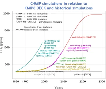
The simulations required for C4MIP are summarized in Table 1 and the CO2concentration is shown schematically in
Fig. 1 in the context of the CMIP6 DECK, historical simu-lations, and the ssp585 future scenario, which is a tier 1 ex-periment of the ScenarioMIP (O’Neill et al., 2016). Table 2 shows the main simulations from other MIPs, which form crucial counterparts to C4MIP simulations. The rest of this section documents detailed instructions on how to set up and perform the C4MIP simulations. Detailed definitions of the output requirements are listed in Sect. 4.
3.2 Experimental details
3.2.1 Model requirements and spin-up
To participate in C4MIP a climate model must have the ca-pability to run with an interactive carbon cycle. This means it must simulate both terrestrial and marine carbon cycle pro-cesses, and it must simulate the exchange of CO2 between
the land/ocean and the atmosphere in order to prognostically
Figure 1. Relation of C4MIP simulations to CMIP6 DECK and his-torical simulations and the ssp585 and ssp5-34-over future scenario simulation proposed for the ScenarioMIP. Note that at the time of preparing this manuscript the details of the SSP5-3.4-OS-Ext exten-sion to 2300 are not available; hence, it could not be included in the figure, but it is still requested as a C4MIP tier-2 simulation.
simulate the evolution of atmospheric CO2. Some C4MIP
simulations prescribe a concentration of CO2 in the
atmo-sphere as a boundary condition and simulate the changes in carbon fluxes and stores in response. Other simulations pre-scribe emissions of CO2to the atmosphere (from human
ac-tivity) as an external forcing and require the model to also simulate the evolution of atmospheric CO2. A model must
be able to run in both these configurations in order to per-form the C4MIP simulations. The evolution of atmospheric CO2concentration can be simulated by assuming that CO2is
completely well mixed with the same globally averaged con-centration everywhere in space or by transporting CO2as a
three-dimensional tracer. This choice is up to the modelling groups. Throughout this document we refer to the former – prescribing atmospheric CO2 concentration as a boundary
condition – as a “concentration-driven” simulation, and the latter – prescribing emissions and in turn simulating the CO2
concentration – as an “emissions driven” simulation. IPCC AR5 WG1 Ch.6 Box 6.4 described the use of these config-urations in some detail (Ciais et al., 2013). Figure 6.4 from that Box is reproduced here for reference (Fig. 2). Although the same terminology (concentration-driven or emissions-driven) can be applied to aerosols or non-CO2 GHGs this
paper focuses only on CO2.
Before beginning the simulations described below, a model must be spun-up to eliminate any long-term drift in carbon stores or fluxes. Indeed, it has been shown recently that the large diversity in spin-up protocols used for marine biogeochemistry in CMIP5 ESMs contribute to large model-to-model differences in simulated fields, and that drifts have
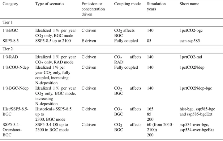
Table 1. Summary of the C4MIP tier-1 and tier-2 simulations. Simulations can be “concentration driven” or “emissions driven” as described in the text. Coupling mode refers to which model components see changes in atmospheric CO2.
Category Type of scenario Emission or concentration driven
Coupling mode Simulation years
Short name
Tier 1
1 %BGC Idealized 1 % per year CO2only, BGC mode
C driven CO2affects
BGC
140 1pctCO2-bgc SSP5-8.5 SSP5-8.5 up to 2100 E driven Fully coupled 85 esm-ssp585 Tier 2
1 %RAD Idealized 1 % per year CO2only, RAD mode
C driven CO2 affects RAD
140 1pctCO2-rad 1 %COU-Ndep Idealized 1 % per
year CO2only, fully
coupled, increasing N-deposition
C driven Fully coupled 140 1pctCO2Ndep
1 %BGC-Ndep Idealized 1 % per year CO2only, BGC mode, increasing N-deposition C driven CO2 affects BGC 140 1pctCO2Ndep-bgc Hist/SSP5-8.5-BGC Historical+SSP5-8.5 up to 2300, BGC mode C driven CO2 affects BGC 165 85 200 hist-bgc, ssp585-bgc and ssp585-bgcExt SSP5-3.4- Overshoot-BGC SSP5-3.4-OS up to 2300 in BGC mode C driven CO2 affects BGC 60 (from 2040– 2100) 200 ssp534-over-bgc, ssp534-over-bgcExt
potential implications on model performance assessments in addition to possibly aliasing estimates of climate change impacts (Séférian et al., 2016). Separate spin-up simula-tions should be performed for both concentration-driven and emission-driven configurations. There are many possi-ble techniques to ensure that a model’s carbon fluxes and pools exhibit minimal drift. These include simply performing very long simulations, running components offline from the coupled system, numerical acceleration techniques or semi-analytical schemes such as described by Xia et al. (2012). The choice of technique is up to the modelling groups and there is no requirement to submit data from the spin-up pe-riod, but a proper documentation of the spin-up technique and duration is required. The test of whether a model is spun-up properly and exhibits minimal drift will be based on the performance of the piControl simulation. It is suggested that the model first be spun-up in concentration-driven mode and this state can be used as an initial basis for the emission-driven spin-up.
Our definition of an acceptably small drift in a properly spun-up model is that land, ocean, and atmosphere carbon stores each vary by less than 10 PgC/century (i.e., a long-term average ≤ 0.1 PgC yr−1). This is broadly equivalent to an atmospheric CO2 drift of less than about 5 ppm/century.
We suggest that a drift smaller than this value is highly
de-sirable but this value is a guideline. Exceeding this drift in the control run may preclude a model from being included in a C4MIP analysis, but we would expect that decision to be made on a case-by-case basis. For example, a large ocean drift in a concentration-driven experiment may not preclude analysis of land carbon fluxes and vice-versa. We also stress that being within these drifts is a minimum but not necessar-ily sufficient quality condition. Regional patterns and drifts of stores and fluxes will also be assessed and depending on the analysis may preclude inclusion of a given model’s re-sults.
For simulations of carbon isotopes, spin-up times of many thousands of years or the use of an equivalent fast spin-up technique may be required to eliminate drift, particularly for carbon-14 in ocean carbon and soil carbon. The spin-up tech-nique is left to the modellers’ discretion.
3.2.2 DECK piControl and historical
The pre-industrial control run (piControl) is a required simu-lation of the CMIP DECK, and a prerequisite simusimu-lation for participating in C4MIP. The run begins from a spun-up state as described above and all forcings should continue to be ap-plied as per the spin-up. The global land and ocean carbon stores should not drift by more than 10 PgC/century each. The length of the pre-industrial control run should be at least
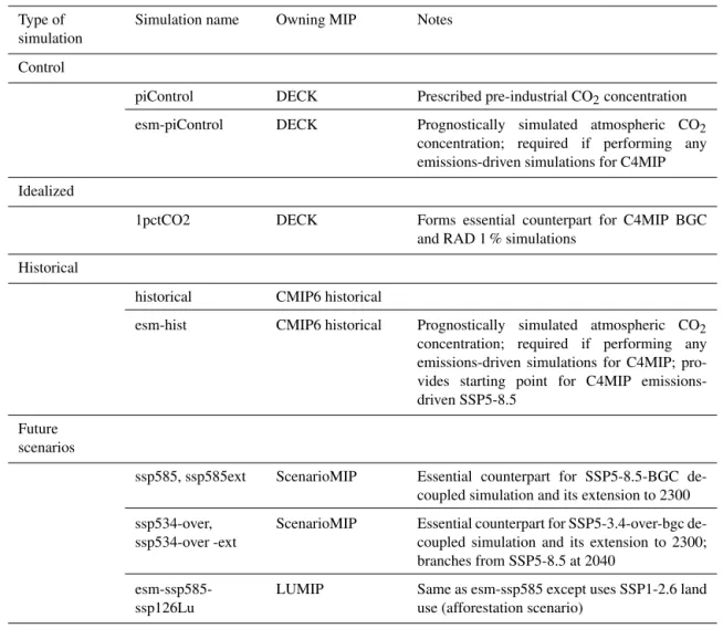
Table 2. Summary of key simulations from CMIP6 DECK, historical or other MIPs on which C4MIP analysis will rely. The emissions-driven control and historical runs in particular are entry card requirements for C4MIP.
Type of simulation
Simulation name Owning MIP Notes
Control
piControl DECK Prescribed pre-industrial CO2concentration
esm-piControl DECK Prognostically simulated atmospheric CO2
concentration; required if performing any emissions-driven simulations for C4MIP Idealized
1pctCO2 DECK Forms essential counterpart for C4MIP BGC and RAD 1 % simulations
Historical
historical CMIP6 historical
esm-hist CMIP6 historical Prognostically simulated atmospheric CO2 concentration; required if performing any emissions-driven simulations for C4MIP; pro-vides starting point for C4MIP emissions-driven SSP5-8.5
Future scenarios
ssp585, ssp585ext ScenarioMIP Essential counterpart for SSP5-8.5-BGC de-coupled simulation and its extension to 2300 ssp534-over,
ssp534-over -ext
ScenarioMIP Essential counterpart for SSP5-3.4-over-bgc de-coupled simulation and its extension to 2300; branches from SSP5-8.5 at 2040
esm-ssp585-ssp126Lu
LUMIP Same as esm-ssp585 except uses SSP1-2.6 land use (afforestation scenario)
equal to any simulation for which it will serve as the control simulation thereby allowing correction for model drift. The piControl run must be run for both concentration-driven and emission-driven configurations of the model. In both cases all forcings should be held constant at pre-industrial levels as described in the CMIP DECK documentation. The only dif-ference between concentration-driven and emission-driven control runs is that the emission-driven simulation simulates atmospheric CO2internally in response to natural fluxes of
carbon from land and ocean, whereas in the concentration-driven case atmospheric CO2concentration is specified. No
anthropogenic fossil fuel emissions of CO2should be applied
to the model during this control run, and fixed pre-industrial land-use should be imposed. The simulated atmospheric CO2
in esm-piControl should therefore remain stable, with drifts below 5 ppm/century.
The CMIP6 historical run, a CMIP6 required simula-tion, must be performed in both concentration-driven and emission-driven configurations for participation in C4MIP. It is expected that the historical simulation would begin
from the same starting point as the pre-industrial control run (Fig. 3). This nominally is set as 1 January 1850. We note though that this neglects the small but non-zero ef-fect of pre-1850 land-use changes (see e.g., Pongratz et al., 2009; Sentman et al., 2011). Some modelling groups might therefore opt for an earlier starting date or perform addi-tional offline land-surface simulations in order to account for pre-1850 land cover change. This would mean though that the control and historical simulations begin from dif-ferent states and with difdif-ferent trends and this should there-fore be very clearly documented. The protocol for the his-torical simulation is documented in detail in the CMIP6 paper (Eyring et al., 2016a). Here we stress the need for the emission-driven historical run (esm-hist) to also be per-formed as an “entry card” for C4MIP. The only difference be-tween concentration-driven and emission-driven simulations is the treatment of atmospheric CO2. All other forcings must
be identical in both simulations. The concentration-driven simulation will use historical atmospheric CO2concentration
Figure 2. Schematic representation of carbon cycle numerical ex-perimental design. Concentration-driven (left) and emissions-driven (right) simulation experiments make use of the same Earth system models (ESMs), but configured differently. Concentration-driven simulations prescribe atmospheric CO2 as a pre-defined input to the climate and carbon cycle model components. Compatible emis-sions can be calculated from the output of the concentration-driven simulations. Emissions-driven simulations prescribe CO2emissions
as the input, and atmospheric CO2is an internally calculated state
variable within the ESM. Adapted from Ciais et al. (2013). Solid arrows depict internal data flow within the model, dashed arrows depict data output from the model.
The emission-driven simulation will use anthropogenic CO2 emissions documented here. Model groups have a
choice over the treatment of land-use forcing as described below.
– Fossil fuel emissions: CMIP6 will provide gridded, an-nual CO2emissions from burning of fossil fuels, from
the beginning of 1850 to the end of 2014 for the his-torical simulation and through to the end of 2100 for ssp5-8.5. See Sect. 3.3.1.
– Land-use carbon emissions: there are two allowable op-tions:
– If possible, drive the model with the CMIP6 land-use forcing (Hurtt et al., 2016; http://luh.umd.edu/ _LUH2/LUH2_1.0h/) and the model simulates its own CO2emissions (including both from
deforesta-tion and uptake from regrowth) to/from the atmo-sphere as an internal process. In this case the only external input of carbon to the system is fossil fuel emissions.
– If that is not possible for the model, then C4MIP will provide land-use carbon emissions; see Sect. 3.3.1.
Figure 3. Schematic representation of model spin-up followed by control and historical simulations through 2014. The interactive CO2pre-industrial control should ideally have a drift of less than
5 ppm/century.
3.2.3 Idealized 1 % simulations
A concentration-driven simulation with a 1 % per year in-crease in atmospheric CO2 concentration beginning from
pre-industrial is a required simulation of the DECK. In C4MIP there are further variants of this 1 % simulation de-signed to quantify the concentration-carbon and climate– carbon feedback parameters (Friedlingstein et al., 2006; Arora et al., 2013).
The tier-1 C4MIP simulation 1pctCO2-bgc requires the simulation to be repeated but with a change to the model set-up such that only the model’s carbon cycle compo-nents (both land and ocean) respond to the increase in CO2,
whereas the model’s radiation code uses a constant, pre-industrial concentration of CO2. This simulation was
previ-ously known as “Uncoupled” in Friedlingstein et al. (2006), and was re-named “Biogeochemically coupled” by Gregory et al. (2009). All other forcings must be identical to the DECK 1pctCO2 simulation.
A tier-2 C4MIP simulation 1pctCO2-rad is the counterpart of 1pctCO2-bgc. It requires the simulation to be repeated but with a change to the model set-up such that only the model’s radiation code sees the increase in CO2and the model’s
car-bon cycle components (both land and ocean) see a constant, pre-industrial concentration of CO2. This simulation was not
performed in Friedlingstein et al. (2006), and was termed “Radiatively coupled” by Gregory et al. (2009). All other forcings must be identical to the DECK 1pctCO2 simula-tion. Although this simulation is in tier-2 we strongly encour-age all modelling groups to perform it as the non-linearities
of biogeochemical and radiative response can be large (e.g. Schwinger et al., 2014).
For models with a nitrogen cycle, there are two fur-ther 1 % simulation variants requested as C4MIP tier-2: 1pctCO2Ndep and 1pctCO2Ndep-bgc. These can be run if the model includes either land- or marine nitrogen cycle in a way that changes carbon uptake and storage. If the input of reactive nitrogen to the model will not affect the car-bon cycle, then there is no need to perform these simula-tions. If changes in nitrogen deposition will affect either land or ocean carbon uptake then these simulations are re-quested. 1pctCO2Ndep and 1pctCO2Ndep-bgc are parallel to the 1pctCO2 and 1pctCO2-bgc simulations but with the addition of a time-varying deposition of reactive nitrogen (see Sect. 3.3.3).
3.2.4 Scenario simulations
Concentration-driven scenario simulations, which follow on from the end of the concentration-driven historical simula-tion, are performed under ScenarioMIP. In C4MIP we re-quest simulations that complement some of these.
Under C4MIP tier-1, we request an emission-driven esm-ssp585 simulation, which parallels the ScenarioMIP concentration-driven SSP-5-8.5 simulation. This simulation should begin from the end point of the emissions-driven his-torical simulation (1 January 2015). As with the hishis-torical simulation the only difference from the concentration-driven counterpart should be the treatment of atmospheric CO2,
which is simulated within the model driven by prescribed emissions. SSP8.5 gridded fossil fuel emissions will be pro-vided as will SSP8.5 land-use forcing and land-use CO2
emissions. Models should implement these in the scenario run in exactly the same manner as they did in the emission-driven historical simulation.
Under C4MIP tier-2, we also request a biogeochemically coupled (BGC) version of the concentration-driven SSP5-8.5, ssp585-bgc and ssp585-bgcExt. As with the 1pctCO2-bgc simulation, this run should be performed with only the carbon cycle components (land and ocean) seeing the pre-scribed increase in atmospheric CO2. The model’s radiation
scheme should see fixed pre-industrial CO2. All other
non-CO2 forcings should be applied in an identical way to the
ScenarioMIP SSP5-8.5 and SSP5-8.5ext simulations. If pos-sible this simulation should be extended to 2300, as should its counterpart from ScenarioMIP, as one of the priority fo-cus areas for analysis is on long-term processes such as ocean carbon and heat uptake and permafrost loss (e.g., Randerson et al., 2015).
3.3 Forcings and inputs
3.3.1 CO2concentrations and anthropogenic CO2
emissions
For concentration-driven simulations, atmospheric CO2
should be prescribed as a globally well-mixed value provided by CMIP6. The CMIP6 paper (Eyring et al., 2016a) and a range of papers in the GMD CMIP6 Special Issue will docu-ment the forcings in more detail. The data will be made avail-able from the CMIP6 and PCMDI webpages (http://www. wcrp-climate.org/wgcm-cmip/wgcm-cmip6, https://pcmdi. llnl.gov/search/input4mips). For emissions-driven simula-tions, atmospheric CO2should be simulated prognostically
by the model. External boundary conditions of anthro-pogenic CO2emissions will be provided and should be used
as follows:
– In esmPIcontrol, the emissions-driven control run, at-mospheric CO2should be simulated by the model but
no external emissions should be added during this sim-ulation.
– Fossil fuel emissions should be used for the emissions-driven historical and future scenario simulations. C4MIP will provide gridded, annual CO2 emissions
from burning of fossil fuels, from the beginning of 1850 to the end of 2014 for the historical simulation and through to the end of 2100 for ssp5-8.5. They will be provided on land points on a 1◦×1◦ grid. It is up to model groups to re-grid or interpolate these emissions to suit their own model. Global annual totals must be conserved and must match the global annual totals of the gridded data provided. Conserving the global annual total is more important than the spatial patterns of emis-sions.
– C4MIP strongly recommends that land-use carbon emissions are simulated internally by applying the land-use forcing by Hurtt et al. (2016). In the event that this is not possible in a model, C4MIP will provide annual land-use carbon emissions mainly based on the results of two bookkeeping models: BLUE (Hansis et al., 2015) and Houghton (Houghton et al., 2012). For the years 1850 to 2010 the average result of these two bookkeep-ing models defines the global emission rate, whereas the spatial distribution of the emissions is taken solely from BLUE at a 0.5◦resolution. This approach provides
in-put emissions more spatially consistent with the land-use forcing applied to models than population-weighted spatial patterns used in CMIP5. For the years 2010 to 2014 the global land-use emission rate is specified by the Global Carbon Project (Le Quéré et al., 2015) and the spatial pattern is that of BLUE at the year 2010. At the time of writing this C4MIP protocol, future land-use scenarios have not yet been processed within LUH2.
Our intention is that for the future scenarios we will provide gridded land-use emissions using global totals from the scenario and the spatial pattern either provided from the scenario or from the BLUE spatial pattern for 2010. As with fossil fuel emissions, it is up to model groups to re-grid or interpolate these emissions to suit their own model. Global annual totals must be con-served and must match the global annual totals of the gridded data provided.
3.3.2 Land-use and land-use-induced land cover change
LULCC affects climate via two aspects in CMIP6 simula-tions. In both concentration-driven and emission-driven sim-ulations LULCC alters the distribution of vegetation cover-ing the land surface, with consequences for the exchange of heat, water, and momentum with the atmosphere. Its ef-fects on terrestrial carbon stocks allow us to infer LULCC emissions, more accurately labelled the “et LULCC flux” (Brovkin et al., 2013). In emission-driven simulations the net LULCC flux influences the atmospheric CO2
concentra-tion, contributing to subsequent carbon cycle feedbacks (e.g., Strassmann et al., 2008; Arora and Boer, 2010; Pongratz et al., 2014).
The LULCC forcing for the historical simulations will be based on the protocol and forcing data provided by CMIP6 for the DECK and the historical CMIP6 simulations. LULCC is kept fixed at its pre-industrial state for all 1pctCO2 simu-lations (fully coupled, biogeochemically and radiatively pled versions). It is essential that the biogeochemically cou-pled simulations required for C4MIP of the historical and fu-ture SSP simulations and their extensions to 2300 use iden-tically the same LULCC forcing as for the parallel Scenari-oMIP simulations.
3.3.3 N deposition
Models including a nitrogen cycle are encouraged to use a consistent set of forcings of anthropogenic nitrogen depo-sition as drivers for the respective ocean and land biogeo-chemical components. Rates of speciated nitrogen deposi-tion at the land and ocean surface are not available from ob-servations and so need to be determined by models. C4MIP will coordinate with CCMI to provide gridded, time-varying fields of nitrogen deposition from chemistry transport models (CTMs) for use as driving inputs in C4MIP simulations (http: //www.met.reading.ac.uk/ccmi/?page_id=375). This will be provided partitioned into four categories of wet or dry and oxidized or reduced N deposition velocities at the bottom of the atmosphere. If a model requires more or fewer categories or species of nitrogen deposition then it is up to the model group to produce these. When aggregating or disaggregating components of deposition the total amount of reactive nitro-gen should be conserved. Inputs into the land biosphere
de-pend on vegetation characteristics, and these aspects should be dealt with by the individual model groups.
C4MIP simulations should use N deposition fields as fol-lows:
– Pre-industrial control (piControl and esm-piControl) should use time-invariant, but spatially explicit, N de-position appropriate to 1850. This is so that there are no discontinuities in carbon pools or fluxes at the beginning of the historical simulation.
– Historical (historical, esm-hist, hist-bgc) and future scenarios (esm-ssp585, ssp585-bgc, ssp585-bgcExt, ssp534-over-bgc, ssp534-over-bgcExt) should use the provided time-varying N-deposition data derived from CTM simulations. It is essential that all C4MIP simu-lations use identically the same N-deposition fields for the C4MIP simulations as the parallel DECK, historical and ScenarioMIP simulations.
– The idealized simulations (1pctCO2, 1pctCO2-bgc, 1pctCO2-rad) should also use the time-invariant pre-industrial N deposition as used in the control runs, as CO2 is the only time-varying forcing in these
experi-ments.
– For the first time, C4MIP requests additional ideal-ized simulations (1pctCO2Ndep, 1pctCO2Ndep-bgc) designed to quantify the effect of N deposition on the carbon–climate and carbon-concentration interactions. These simulations should use an idealized scenario of time-varying N deposition as follows. A scenario will be generated by adding to the pre-industrial base-line the geographically explicit difference between the year 2100 SSP5-8.5 N deposition scenario and pre-industrial values, such that the relative growth rates of N deposi-tion and CO2 match and the global total N deposition
at the time when atmospheric CO2concentrations reach
the SSP5-8.5 value for the year 2100 correspond to the year 2100 N deposition total. C4MIP will generate these fields of N deposition and make them available as an-nual fields to be applied in these idealized simulations. If the ESM simulates atmospheric chemistry and composi-tion and therefore provides N deposicomposi-tion internally, then this can be used in place of a prescribed field of N deposition for the control, historical, and scenario simulations. However, ir-respective of whether an ESM generates N deposition or not, for the 1 % idealized simulations, it is preferable to use the provided fields as anomalies, which should be added to the ESM’s pre-industrial N-deposition fields.
The provided N-deposition data will cover both land and ocean, but we acknowledge that some models have their own established sources of reactive nitrogen to the oceans and to change this would require costly repeat-spinup simulations. So it is left to the model groups’ discretion how to apply N deposition to the ocean. If a source other than that provided
1860 1880 1900 1920 1940 1960 1980 2000 −8.5 −8 −7.5 −7 −6.5 1860 1880 1900 1920 1940 1960 1980 2000 0 200 400 600 800 NH Trop SH Atmospheric ∆14CO 2 Atmospheric δ13CO 2 δ 13C (‰) ∆ 14C (‰)
Figure 4. Carbon isotopes in atmospheric CO2for the historical
period 1850–2014. Data for δ13C is from Law Dome, South Pole (Rubino et al., 2013), and Mauna Loa (Keeling et al., 2001) and includes smoothing of the observations. Data for 114C are com-piled from Levin et al. (2010) and other sources (I. Levin, personal communication, 2016), following a similar data set used by Orr et al. (2000).
by C4MIP is used this should be documented and made avail-able to aid analyses.
3.3.4 Carbon isotopes
Models including carbon isotopes (δ13C and 114C) in land or ocean realms are encouraged to simulate and report variables relating to carbon isotopes for control, historical, and future scenario simulations.
For historical concentration-driven runs (piControl, histor-ical and hist-bgc), atmospheric δ13CO2and 114CO2forcing
based on observations will be provided (Fig. 4). The atmo-spheric forcing data sets will be available at the C4MIP web-site. We also plan to make available atmospheric forcing data for carbon isotopes for the ssp585 scenario and for other sce-narios and extensions using a simple carbon cycle model, fol-lowing Graven (2015).
Carbon isotopes are only requested to be simulated in land and ocean model components using the provided histori-cal or future atmospheric forcing data sets for δ13CO2and
114CO2. It is not requested that atmospheric δ13CO2 and
114CO2 be simulated by ESMs, even for emission-driven
simulations of atmospheric CO2.
3.3.5 Other forcings
If the model requires any other external forcing not docu-mented here, for example deposition of phosphorous, then it is at the model groups’ discretion how to provide it. In the case of a model with an interactive phosphorous cycle, we recommend the forcing data are prepared in a way analogous to the nitrogen deposition described above. We recommend modelling groups to contact C4MIP for more details if this is applicable. Any additional forcings must be documented through the CMIP meta-data process or in the appropriate model description paper.
4 Output requirements
It is vital for accurate analysis and model intercomparison that every model adheres to the definitions of each output variable in order for a like-for-like comparison to be made. In this section we describe in detail each requested output vari-able. The data request will be documented separately (by the WGCM Infrastructure Panel; https://www.earthsystemcog. org/projects/wip/) and will list the required variables output for each CMIP6 simulation along with their precise variable names, description, and required units. Here we aim to de-scribe each variable so that its implementation and use are made consistent across all models and analyses.
4.1 Land
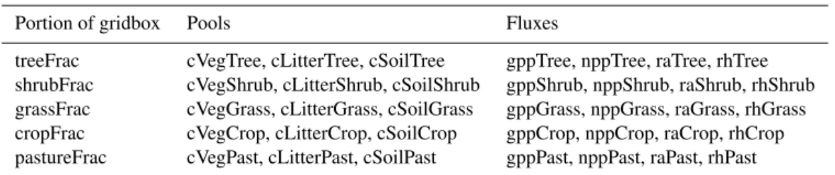
4.1.1 Land carbon cycle variables
The primary aim of C4MIP is to compare the aspects of the global carbon cycle and its response to environmental changes across the participating ESMs. To achieve this ob-jective, it is essential that all carbon stocks and fluxes are reported so that total amount of carbon in the system can be tracked and their conservation checked. To achieve this, compulsory tier-1 diagnostics have been defined that close the carbon cycle as simply as possible. Desirable tier-2 diag-nostics should also be reported where possible, which allow for more detailed analysis by breaking down tier-1 output into sub-components.
Land carbon pools: tier-1
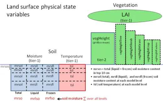
Figure 5 shows the requested carbon cycle stores over land. Tier-1 variables are intended to be simple but still capture the total land carbon store. Tier-2 variables provide the same in-formation as the tier-1 variables but in more detail. As shown in Fig. 5 the total carbon can be calculated from tier-1 ables and is not the combined sum of tier-1 and tier-2 vari-ables.
The carbon stored in the vegetation–litter–soil system is simply represented by tier-1 variables, cVeg, cLitter, and cSoil respectively. For models that do not
repre-Figure 5. (a) Requested tier-1 and tier-2 variables representing land carbon pools. Although not a land carbon quantity, atmospheric CO2
is shown here for completeness. (b) Detailed view of the tier-2 breakdown for soil carbon by vertical level (cSoilLevels) and by soil carbon pool (cSoilPools).
sent a vertical discretization of soil carbon, all soil car-bon should be reported simply as cSoil. Additionally in tier-1 for models with vertically discretized soil car-bon, we request output on the vertical distribution above and below 1 m depth (cSoilAbove1m, cSoilBelow1m). These should be reported in addition to cSoil, such that cSoil=cSoilAbove1m+cSoilBelow1m. The rationale for re-questing this is the availability of several observation-based data sets that report soil organic matter content to 1 m depth. It is important that any evaluation of cSoil outputs against observed data sets makes use of the appropriate depth of soil in both the observations and model outputs.
A fourth pool, cProduct, represents the carbon stored in product pools (harvested wood, paper products, furniture, etc.) as a result of anthropogenic land-use change. The to-tal carbon stored per unit area on land is then simply: cLand = cVeg + cLitter + cSoil + cProduct (1) Some models may not explicitly simulate a litter pool distinct from their soil carbon pool. In this case cLitter should be re-ported as zero. We would normally expect cProduct to be non-zero in simulations that include anthropogenic land-use or land-use change. Hence, for the idealized 1 % per year in-creasing CO2 simulations (biogeochemically, radiatively or
fully coupled) we would expect models to report cProduct = 0. For models whose land-use fluxes contribute straight to the atmosphere and/or to their litter or soil carbon pools, but not to the product pools, cProduct = 0 should also be reported for historical and scenario simulations. Obviously, for mod-els that do not simulate the effect of LULCC on the carbon cycle, cProduct will also be expected to be zero.
Land carbon pools: tier-2 vegetation and litter carbon Tier-2 output variables allow for more detailed breakdown and analysis of their parent carbon stores. They are sub-components of their parent tier-1 variables, and not addi-tional stores. For example, the vegetation carbon pool can be represented by carbon in the leaf, stem, and root as well as possibly other (e.g. fruit) components. For models that re-port these tier-2 variables, the total amount of carbon per unit area should be identical to the tier-1 variable, i.e.
cVeg = cLeaf + cStem + cRoot + cOther. (2) The same applies for the litter carbon pool, which is re-quested to be broken down into coarse woody debris (cLitter-CWD) and above- and below-surface litter (cLitterSurf, cLit-terSubSurf) pools. When a model has a continuous profile of litter with depth, take above and below 10 cm as the defini-tion of above and below the surface. CWD here is assumed to be on the surface.
Land carbon pools: tier-2 soil carbon
For CMIP5 the soil carbon pool was requested to be di-vided into components with fast, medium, and slow turnover timescales. However, this distinction was not found useful by the community and as a result was not used in many anal-yses. For CMIP6, we request a breakdown in two different ways (Fig. 5b). First, models with a vertical structure to their soil carbon are requested to report total soil carbon for each soil layer. In the same way as soil moisture or temperature, this should be reported as a multi-level output, cSoilLevels. As the structure for this may vary between models, it is es-sential that the model is thoroughly documented. The sum of soil carbon over all cSoilLevels should be identical to the total cSoil tier-1 variable.