HAL Id: hal-00328468
https://hal.archives-ouvertes.fr/hal-00328468
Submitted on 16 Nov 2006
HAL is a multi-disciplinary open access
archive for the deposit and dissemination of
sci-entific research documents, whether they are
pub-lished or not. The documents may come from
teaching and research institutions in France or
abroad, or from public or private research centers.
L’archive ouverte pluridisciplinaire HAL, est
destinée au dépôt et à la diffusion de documents
scientifiques de niveau recherche, publiés ou non,
émanant des établissements d’enseignement et de
recherche français ou étrangers, des laboratoires
publics ou privés.
AeroCom present-day and pre-industrial simulations
M. Schulz, C. Textor, S. Kinne, Yves Balkanski, S. Bauer, T. Berntsen, T.
Berglen, O. Boucher, F. Dentener, S. Guibert, et al.
To cite this version:
M. Schulz, C. Textor, S. Kinne, Yves Balkanski, S. Bauer, et al.. Radiative forcing by aerosols
as derived from the AeroCom present-day and pre-industrial simulations. Atmospheric Chemistry
and Physics, European Geosciences Union, 2006, 6 (12), pp.5246. �10.5194/acp-6-5225-2006�.
�hal-00328468�
www.atmos-chem-phys.net/6/5225/2006/ © Author(s) 2006. This work is licensed under a Creative Commons License.
Chemistry
and Physics
Radiative forcing by aerosols as derived from the AeroCom
present-day and pre-industrial simulations
M. Schulz1, C. Textor1, S. Kinne2, Y. Balkanski1, S. Bauer3, T. Berntsen4, T. Berglen4, O. Boucher5,11, F. Dentener6, S. Guibert1, I. S. A. Isaksen4, T. Iversen4, D. Koch3, A. Kirkev˚ag4, X. Liu7,12, V. Montanaro8, G. Myhre4,
J. E. Penner7, G. Pitari8, S. Reddy9, Ø. Seland4, P. Stier2, and T. Takemura10
1Laboratoire des Sciences du Climat et de l’Environnement, CEA-CNRS-UVSQ, Gif-sur-Yvette, France
2Max-Planck-Institut f¨ur Meteorologie, Centre for Marine and Atmospheric Sciences (ZMAW), Hamburg, Germany 3Columbia University, GISS, New York, USA
4University of Oslo, Department of Geosciences, Oslo, Norway 5Hadley Centre, Met Office, Exeter, UK
6European Commission, Joint Research Centre, Institute for Environment and Sustainability,Climate Change Unit, Ispra, Italy 7Department of Atmospheric, Oceanic and Space Sciences, University of Michigan, Ann Arbor, MI, USA
8Dipartimento di Fisica, Universit`a degli Studi L’Aquila, Coppito, Italy
9NOAA, Geophysical Fluid Dynamics Laboratory, Princeton, New Jersey, USA 10Research Institute for Apllied mechanics, Kyushu University, Fukuoka, Japan
11Laboratoire d’Optique Atmospherique, Universit´e des Sciences et Technologies de Lille, CNRS, Villeneuve d’Ascq, France 12Battelle, Pacific Northwest National Laboratory, Richland, WA, USA
Received: 25 April 2006 – Published in Atmos. Chem. Phys. Discuss.: 22 June 2006 Revised: 17 October 2006 – Accepted: 22 October 2006 – Published: 16 November 2006
Abstract. Nine different global models with detailed aerosol modules have independently produced instantaneous direct radiative forcing due to anthropogenic aerosols. The an-thropogenic impact is derived from the difference of two model simulations with prescribed aerosol emissions, one for present-day and one for pre-industrial conditions. The differ-ence in the solar energy budget at the top of the atmosphere (ToA) yields a new harmonized estimate for the aerosol di-rect radiative forcing (RF) under all-sky conditions. On a global annual basis RF is −0.22 Wm−2, ranging from +0.04 to −0.41 Wm−2, with a standard deviation of ±0.16 Wm−2. Anthropogenic nitrate and dust are not included in this esti-mate. No model shows a significant positive all-sky RF. The corresponding clear-sky RF is −0.68 Wm−2. The cloud-sky RF was derived based on all-sky and clear-sky RF and mod-elled cloud cover. It was significantly different from zero and ranged between −0.16 and +0.34 Wm−2. A sensitivity anal-ysis shows that the total aerosol RF is influenced by consid-erable diversity in simulated residence times, mass extinction coefficients and most importantly forcing efficiencies (forc-ing per unit optical depth). The clear-sky forc(forc-ing efficiency (forcing per unit optical depth) has diversity comparable to that for the all-sky/ clear-sky forcing ratio. While the di-versity in clear-sky forcing efficiency is impacted by factors
Correspondence to:M. Schulz
(michael.schulz@cea.fr)
such as aerosol absorption, size, and surface albedo, we can show that the all-sky/clear-sky forcing ratio is important be-cause all-sky forcing estimates require proper representation of cloud fields and the correct relative altitude placement be-tween absorbing aerosol and clouds. The analysis of the sul-phate RF shows that long sulsul-phate residence times are com-pensated by low mass extinction coefficients and vice versa. This is explained by more sulphate particle humidity growth and thus higher extinction in those models where short-lived sulphate is present at lower altitude and vice versa. Solar atmospheric forcing within the atmospheric column is esti-mated at +0.82±0.17 Wm−2. The local annual average max-ima of atmospheric forcing exceed +5 Wm−2confirming the regional character of aerosol impacts on climate. The annual average surface forcing is −1.02±0.23 Wm−2. With the cur-rent uncertainties in the modelling of the radiative forcing due to the direct aerosol effect we show here that an estimate from one model is not sufficient but a combination of several model estimates is necessary to provide a mean and to ex-plore the uncertainty.
1 Introduction
Anthropogenic aerosols modify the Earth radiation budget such that flux changes can be observed by satellites (Bellouin
et al., 2005). Their increased presence since pre-industrial times is suspected to have partly offset global warming in the 20th century (Charlson et al., 1992). This in turn would be responsible for additional climate warming if aerosols were removed in the future through abatement of aerosol related air pollution (Anderson et al., 2003). There is also a sugges-tion that aerosol forcing has an important regional impact on weather and climate (Menon et al., 2002). Reduced incom-ing radiation observed at surface level, called global dim-ming, was associated with the effect of aerosols (Liepert et al., 2004; Stanhill and Cohen, 2001).
Considerable uncertainty in the radiative forcing by the different anthropogenic aerosol components has been sum-marized by IPCC, 2001. The need to integrate the aerosol ef-fects on a global scale has given rise in recent years to the de-velopment of models, in which aerosol modules gained con-siderable complexity (Ghan, 2001; Liao et al., 2004; Martin et al., 2004; Stier et al., 2005). However, models still suf-fer from difficulties in representing the aerosol physics in a sufficiently coherent and complex way so as to reproduce all aspects observed with a wide range of aerosol instruments. The model inter-comparison within the framework of the Ae-roCom initiative (http://nansen.ipsl.jussieu.fr/AEROCOM/) has revealed important differences in describing the aerosol life cycle at all stages from emission to optical properties (Kinne et al., 2006; Textor et al., 2006).
Here we present the results of a joint study of AeroCom models with the aim of deriving a state-of-the-art best guess for the direct radiative forcing (RF) attributable to anthro-pogenic aerosol. With the additional diagnostics available in AeroCom we also aim to analyze the differences in RF between models. Note, this RF does not include indirect forcing contributions by aerosol induced changes to clouds and the hydrological cycle. The RF collected here lacks the contributions from anthropogenic nitrate and dust. Two ex-periments were performed by each of the models based on predefined emission datasets assumed to be representative for pre-industrial times at about 1750 (“AeroCom PRE”) and for the year 2000 (“AeroCom B”) and in principal fixed me-teorological fields representing the year 2000. The differ-ence in radiative energy balance between both experiments defines the impact due to anthropogenic aerosol. This defi-nition also captures the effect of any non-linear aerosol dy-namics, when anthropogenic aerosol interacts with the nat-ural aerosol background, and when the anthropogenic com-ponents itself are present to a varying degree in present and pre-industrial situations. Such interactions are simulated in varying degree of complexity by the nine models as detailed by Textor et al. (2006). We note finally here that in this study we prescribed the emissions: the uncertainties in the emis-sion datasets would add to the over-all uncertainty of our RF calculation.
2 Model simulations 2.1 Experimental setup
The analysis of the model results in this study builds on an open call to aerosol modelling groups to contribute to the Ae-roCom initiative. Three joint experiments (A, B, PRE) have been performed within AeroCom. The original model ver-sions (experiment A) had not included a RF diagnostic but are documented in detail with respect to the aerosol life cy-cle and optical properties by Kinne et al. (2006) and Textor et al. (2006). Here we analyse the other two simulations where aerosol emissions have been prescribed for current (exper-iment B) and pre-industrial conditions (exper(exper-iment PRE). Otherwise these experiments should not differ from A, but included additional diagnostics on RF. Groups were asked to provide output according to a protocol available on the AeroCom website (http://nansen.ipsl.jussieu.fr/AEROCOM/ protocol.html). Nine (of the sixteen) AeroCom models con-tributed their RF results for experiments B and PRE along with the diagnostics retrieved already for experiment A. Ta-ble 1 lists the models, their abbreviations and references to publications that provide more detail. Initial checks of the received output were conducted via an interactive website open to the public (http://nansen.ipsl.jussieu.fr/AEROCOM/ data.html). The parameters gathered comprise daily values for RF at the top of the atmosphere and at the surface, plus associated data on aerosol properties (mass loading, opti-cal depth, size, absorption, single scattering albedo, altitude, component mass extinction efficiencies) and on environmen-tal properties (solar surface albedo and cloud distribution). For both experiments AeroCom B and AeroCom PRE the modelers were asked to use a priori the analyzed meteoro-logical fields for the year 2000 to either drive or nudge their model. This was done to obtain results corresponding to the AeroCom A experiment, where modelers used emissions of their choice, and which were analyzed in the above men-tioned overview publications. The two participating mod-els without nudging capability (UIO GCM and ULAQ) es-tablished climatological means based on a 5-year simulation after a spin-up period of one year.
As has been done already in Textor et al. (2006), we define model diversity as the standard deviation among the model results. This allows to easily compare the results with those from Textor et al. (2006). Note our estimate of the standard deviation is based on only 9 AeroCom models. In addition to analysing the nine AeroCom model results incorporated in the present study on their original grid we also present fig-ures from an average AeroCom model, constructed from the outputs of the nine models. For this purpose only the origi-nal data were re-gridded by interpolation to a common grid of horizontal resolution of 1×1 degree latitude/longitude. A local diversity diagnostic at any grid point is calculated as the standard deviation from the values of the nine models.
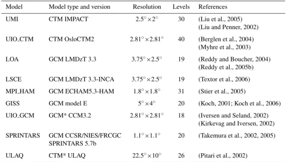
Table 1. Model names and corresponding models and version names, their resolution used here and selected principal publications associated to each model. See also Textor et al. (2006) for more complete descriptions of the models. “*” signifies a climatological model was run for a five year period. All other models are driven by analysed meteorological fields (nudged climate model or chemical transport model).
Model Model type and version Resolution Levels References UMI CTM IMPACT 2.5◦×2◦ 30 (Liu et al., 2005)
(Liu and Penner, 2002) UIO CTM CTM OsloCTM2 2.81◦×2.81◦ 40 (Berglen et al., 2004)
(Myhre et al., 2003) LOA GCM LMDzT 3.3 3.75◦×2.5◦ 19 (Reddy and Boucher, 2004)
(Reddy et al., 2005b) LSCE GCM LMDzT 3.3-INCA 3.75◦×2.5◦ 19 (Textor et al., 2006)
MPI HAM GCM ECHAM5.3-HAM 1.8◦×1.8◦ 31 (Stier et al., 2005)
GISS GCM model E 5◦×4◦ 20 (Koch, 2001; Koch et al., 2006)
UIO GCM GCM* CCM3.2 2.81◦×2.81◦ 18 (Iversen and Seland, 2002)
(Kirkevag and Iversen, 2002) SPRINTARS GCM CCSR/NIES/FRCGC 1.1◦×1.1◦ 20 (Takemura et al., 2002, 2005)
SPRINTARS 5.7b
ULAQ CTM* ULAQ 22.5◦×10◦ 26 (Pitari et al., 2002)
The interpolation served also for comparison to satellite data products shown e.g. in Kinne et al. (2006).
2.2 AeroCom emission datasets
Inventories for global emissions of aerosol and pre-cursor gases for the years 2000 (current conditions) and 1750 (pre-industrial conditions) were established based on available data in 2003. All emissions data-sets are available via a file transfer site at the Joint Research Center (JRC), Italy: ftp://ftp.ei.jrc.it/pub/Aerocom/. Here, we give a very brief description and the reader is referred to (Dentener et al., 2006) for more detailed information. Dust, sea-salt, sulphur components and carbonaceous aerosol emissions are pro-vided at a spatial resolution of 1◦×1◦. Temporal resolution ranges from daily for dust, sea salt and DMS to yearly for the remaining constituents. The injection altitudes and the size of the injected particles of emissions are prescribed. Aerosol emissions are categorized by its origin into “natural” and “anthropogenically modified”. Natural emissions of sea-salt, dust, DMS, secondary organic aerosol and volcanic activity are assumed identical for current and pre-industrial condi-tions. Anthropogenically modified emissions consider con-tributions to sulphur (S), Particulate Organic Matter (POM) and Black (or elementary) Carbon (BC) from large scale wild-land fires (partly natural), bio fuel burning and fossil fuel burning. For pre-industrial times contributions from wild-land fires (open burning) and biofuel emissions are re-duced and fossil fuels emissions are ignored. In summary we assume anthropogenic emissions for black carbon of
6.32 Tg/year, for particulate organic matter of 32.5 Tg/year and for sulphur dioxide of 100.9 Tg-SO2/year.
2.3 Model simulation of the anthropogenic components and forcing
The RF calculations analysed in this study involve nine dif-ferent model environments with respect to the complexity of the aerosol modules and associated global circulation mod-els. While the reader is encouraged to explore publications describing the individual models (see Table 1) together with the initial AeroCom papers from Textor et al. (2006) and Kinne et al. (2006), we consider it necessary here to docu-ment some of the differences in the RF calculation.
RF is defined as “the change in net (down minus up)
ir-radiance (solar plus long-wave; in Wm−2) at the tropopause
AFTER allowing for stratospheric temperatures to readjust to radiative equilibrium, but with surface and tropospheric
temperatures and state held fixed at the unperturbed values”,
which is exerted by the introduction of a perturbing agent (Ramaswamy et al., 2001). For most aerosol constituents stratospheric adjustment has little effect on the RF, and the instantaneous RF at the top of the atmosphere (ToA) can be substituted for the stratospheric-adjusted RF. AeroCom RF results refer to ToA-RF. With respect to the flux perturbation by the anthropogenic aerosol we suggest here that the unper-turbed state is characterized by experiment AeroCom-PRE. The analysis of the RF differences between models requires that we also retrieve the anthropogenic perturbation for sev-eral other parameters. This has been obtained by subtracting
AeroCom-PRE from AeroCom-B simulation results. Since these are the only useful parameter values to be compared to RF we omit for simplicity in the remainder the specification “anthropogenic” for parameters. “Load” thus refers just to the anthropogenic load, if not mentioned otherwise.
Note that the RF derived from the AeroCom simulations does not include anthropogenic nitrate and dust, since they are not considered in the AeroCom emission database. Ni-trate RF has been suggested to range between −0.03 and −0.22 Wm−2 (Jacobson, 2001a; Adams et al., 2001; Liao and Seinfeld, 2005). Dust RF is potentially more important, if the anthropogenic fraction of dust would be large. Esti-mates for it range from 0% to 50% (Tegen and Fung, 1995; Mahowald and Luo, 2003; Mahowald et al., 2004; Tegen et al., 2004; Moulin and Chiapello, 2004). The radiative effect of anthropogenic dust would be important if the dust radia-tive effect would be largely different from zero. However, the partial absorbing nature of dust particles is difficult to quan-tify and adds important uncertainty to any dust RF estimate (e.g., Haywood et al., 2003; Kaufman et al., 2001; Coen et al., 2004; Huebert et al., 2003; Clarke et al., 2004; Balkanski et al., 2006).
The omission of anthropogenic dust, of which the sources and optical properties are very uncertain, simplifies the RF calculations in that only solar broadband flux changes need to be considered. Recent work (by Reddy et al., 2005a) sug-gests that significant flux changes in the infrared part of the spectrum do not occur in the absence of mineral dust, essen-tially because anthropogenic aerosol other than dust is sub-micron in size. RF results reported here are for the shortwave spectrum only.
A conceptual difference among models in obtaining RF of the anthropogenic aerosol and its components is the choice of the unperturbed reference state. Internal mixing and other interactions between aerosol components affect size distribu-tion and hygroscopicity and result in interdependencies be-tween e.g. the sulphate RF and the black carbon RF. For the total aerosol RF a reference state with natural background aerosol is preferred over a no-aerosol reference. The exper-imental set-up (“B”–“PRE”) establishes this type of a natu-ral aerosol reference, and it guarantees comparability among models for the total anthropogenic (direct aerosol) impact. However, the exact procedure on how to retrieve aerosol component RF differs in between models. One way would be to isolate the perturbation due to a single component by an additional experiment, in addition to “B” and “PRE”, where the target component is absent. MPI HAM simula-tions refer to five experiments on top of a present day refer-ence case to identify separately the RF of sulphate, biomass burning, total carbonaceaous aerosol, fossil fuel carbona-ceous aerosol and total aerosol. Another solution was cho-sen in UIO GCM where the contribution from BC, POM, BC+POM and sulphate are removed in two more experi-ments per species from both present day and pre-industrial simulations. RF is then the difference between two pairs of
simulation: RFx=(B–PRE)–(B−x–PRE−x). Most models do not try to account for non-linear effects resulting from the aerosol mixing state and the impact it has on optical prop-erties and computed the RF of individual components from aerosol component fields established in experiment B against the Reference case PRE. It is beyond the scope of this paper and not documented in the AeroCom dataset how the non-linear effects of aerosol mixing influence the RF results. See for further discussion e.g. Jacobson (2001a), Kirkev˚ag and Iversen (2002), Liao and Seinfeld (2005), Stier et al. (2006a), and Stier et al. (2006b). The consequences of the different ways of describing a reference state are difficult to estimate without dedicated experiments in a single model. The results summarised here involve both model diversity with respect to aerosol properties and RF calculation concept.
Finally, for completeness and also comparability with pub-lished data, we document here deviations from the general methodology described above or from work in publications cited e.g. in Table 1. Note that these deviations are model specific and due rather to technical problems when setting up the AeroCom experiment. The following is thus more a listing and consequences for this study are thought to be small. Since the overall average for these values was negligi-ble they were simply removed from consideration. Deviating from AeroCom experiment A the SPRINTARS model treated black carbon (BC) and particulate organic matter (POM) as external mixture. As compared to experiment A this resulted in lower solubility of the BC and thus extended BC lifetime. The GISS model simulated different concentration fields for natural aerosol (dust and sea-salt) in the two simulations (B and PRE) because heterogeneous concentrations changed e.g. the solubility of dust. This difference was not considered here as contributing to the “anthropogenic” RF term. Nat-ural aerosols differ for the MPI HAM model, where emis-sions of natural aerosol, in place of AeroCom suggestions, were implemented via an interactive source. The UIO GCM model used prescribed sea salt and dust fields (Kirkev˚ag et al., 2005). The ULAQ model reports only clear sky forcing. The all-sky forcing in ULAQ was assumed to be 30% of the clear-sky value (assuming 70% cloud cover and no aerosol forcing in cloudy conditions). The underlying assumption of zero RF in cloudy conditions may be likely wrong if the clear-sky RF is relatively weak and negative globally and positive in large regions. The positive forcing may be magni-fied, not reduced in cloudy conditions. However, looking at the other models with complete information reveals that out of 7 models, 3 suggest negative and 4 neutral or slightly pos-itive cloud-sky-forcing. There is no consensus on the sign of this term of RF. Without further calculations available, we believe that retrieving an all-sky forcing for ULAQ this way serves comparability, even though its use is limited. Note also that the AeroCom average estimate for RF would change just slightly from −0.219 to −0.216 Wm−2if we would omit the ULAQ-RF results.
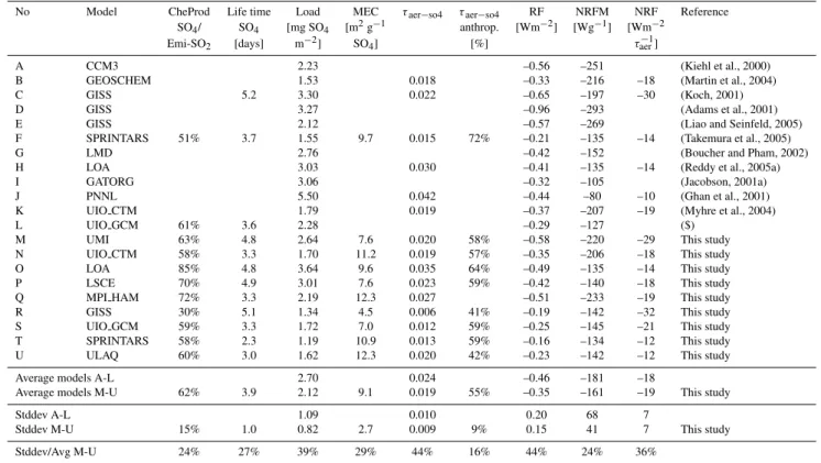
Table 2. Sulphate aerosol forcing related global mean values, derived from recent publications (Models A-L) and from this studies Ae-roCom simulations, using identical emissions (Models M-U). All values refer to the anthropogenic perturbation of atmospheric sulphur. “CheProdSO4/Emi-SO2”: Chemical production of aerosol sulphate over sulphur-emission, both in terms of sulphur mass; “Life time”:
de-rived from sulphate burden and chemical production; “MEC”: mass extinction coefficient dede-rived from dry load and sulphate aerosol optical depth; “τaer−so4and τaer−so4anthrop.”: anthropogenic sulphate aerosol optical depth and its fraction of present day sulphate optical depth; “RF”: shortwave radiative forcing; “NRFM”: normalized RF per load; “NRF”: normalized RF per unit τaer−so4.
No Model CheProd Life time Load MEC τaer−so4 τaer−so4 RF NRFM NRF Reference SO4/ SO4 [mg SO4 [m2g−1 anthrop. [Wm−2] [Wg−1] [Wm−2
Emi-SO2 [days] m−2] SO
4] [%] τaer−1]
A CCM3 2.23 –0.56 –251 (Kiehl et al., 2000)
B GEOSCHEM 1.53 0.018 –0.33 –216 –18 (Martin et al., 2004)
C GISS 5.2 3.30 0.022 –0.65 –197 –30 (Koch, 2001)
D GISS 3.27 –0.96 –293 (Adams et al., 2001)
E GISS 2.12 –0.57 –269 (Liao and Seinfeld, 2005)
F SPRINTARS 51% 3.7 1.55 9.7 0.015 72% –0.21 –135 –14 (Takemura et al., 2005)
G LMD 2.76 –0.42 –152 (Boucher and Pham, 2002)
H LOA 3.03 0.030 –0.41 –135 –14 (Reddy et al., 2005a)
I GATORG 3.06 –0.32 –105 (Jacobson, 2001a)
J PNNL 5.50 0.042 –0.44 –80 –10 (Ghan et al., 2001)
K UIO CTM 1.79 0.019 –0.37 –207 –19 (Myhre et al., 2004)
L UIO GCM 61% 3.6 2.28 –0.29 –127 ($)
M UMI 63% 4.8 2.64 7.6 0.020 58% –0.58 –220 –29 This study
N UIO CTM 58% 3.3 1.70 11.2 0.019 57% –0.35 –206 –18 This study
O LOA 85% 4.8 3.64 9.6 0.035 64% –0.49 –135 –14 This study
P LSCE 70% 4.9 3.01 7.6 0.023 59% –0.42 –140 –18 This study
Q MPI HAM 72% 3.3 2.19 12.3 0.027 –0.51 –233 –19 This study
R GISS 30% 5.1 1.34 4.5 0.006 41% –0.19 –142 –32 This study
S UIO GCM 59% 3.3 1.72 7.0 0.012 59% –0.25 –145 –21 This study
T SPRINTARS 58% 2.3 1.19 10.9 0.013 59% –0.16 –134 –12 This study
U ULAQ 60% 3.0 1.62 12.3 0.020 42% –0.23 –142 –12 This study
Average models A-L 2.70 0.024 –0.46 –181 –18
Average models M-U 62% 3.9 2.12 9.1 0.019 55% –0.35 –161 –19 This study
Stddev A-L 1.09 0.010 0.20 68 7
Stddev M-U 15% 1.0 0.82 2.7 0.009 9% 0.15 41 7 This study
Stddev/Avg M-U 24% 27% 39% 29% 44% 16% 44% 24% 36%
$ Kirkevag and Iversen, 2002; Iversen and Seland, 2002
Most probably there are other differences between models, which we are not aware of. We feel that the methodological deviations documented here illustrate the unavoidable imper-fection of a model intercomparison effort but that might help to guide future research. We note also that a direct com-parison to results from the two accompanying papers Textor et al. (2006) and Kinne et al. (2006) are difficult, because they refer to AeroCom A simulations and the natural and anthropogenic aerosol together, while this paper focuses on the AeroCom B and PRE experiments and the anthropogenic aerosol fraction only.
3 Results
3.1 Sulphate aerosols
Model results for anthropogenic sulphate load, aerosol opti-cal depth (AOD, always in this paper for mid-visible wave-lengths (0.55 µm)) and its fraction with respect to total sul-phate are summarized in Table 2. Also listed in this table are
model predictions for the sulphate RF and associated forcing efficiencies, forcing with respect to sulphate load and AOD, respectively. Results of AeroCom models are found in the lower part of the table and they are compared to previous model predictions, provided in the upper part of the table. Average and standard deviation for the two groups of model results are placed at the bottom of the table to illustrate how much the coordinated AeroCom effort differs from model re-sults found in the published literature.
The AeroCom results and previous model predictions agree that sulphate exerts a negative RF, cooling the Earth-Atmosphere-System. The mean of the RF estimate from the AeroCom models (−0.35 Wm−2) is 25% smaller than those from previous model predictions (−0.46 Wm−2). Both sul-phate burdens and optical depths are 25% smaller for the AeroCom models, suggesting that emissions could be lower in the AeroCom simulations. While we have not all infor-mations available for the previous model predictions we can compare AeroCom A and B results. AeroCom B emissions are on average 10% less than the SO2 emissions used in experiment A. On average, among the nine models
investi-gated here, aerosol load was almost the same between A and B and AOD of sulphate decreased by 5%. Assuming that the AeroCom A set-ups resemble the previous model pre-dictions, this suggests that the revised and regionally shifted SO2emissions (AeroCom B suggests especially reductions in Europe) alone can not explain the difference between the AeroCom results and previous model predictions. Note also, that the mean forcing efficiency with respect to sulphate load (NRFM) from previous model predictions is slightly higher than that of AeroCom, but that the forcing efficiency per unit optical depth is rather similar.
However, RF results from the models still vary substan-tially, reflected by a significant standard deviation (ca. 40% on average) for load, AOD and RF. This diversity is larger than the difference between the averages from the two model groups. The diversity of RF among AeroCom models is only slightly smaller than that of the previous model predictions. A comparison with RF results from AeroCom A simulations is unfortunately not available. However, we can compare the AOD-diversity for the nine AeroCom models between Com A as reported by Kinne et al. (2006) with their Aero-Com B simulations as used here. Mean total sulphate AOD (natural and anthropogenic) and the corresponding diversity as standard deviation was very similar (A: 0.032±44% ver-sus B: 0.030±49%). This altogether suggests that the pre-scribed emissions in AeroCom do not produce a significantly larger agreement among models.
The previous COSAM intercomparison stated in fact simi-lar diversity based on 10 global aerosol models (Barrie et al., 2001) using identical emissions. GISS and MPI HAM ver-sions had already participated in this earlier exercise. Resi-dence times of sulphate in the 10 models in COSAM ranged between 3.2 and 7.5 days, the range being shifted to slightly smaller values in this study (2.3 to 5.1 days). Vertical sul-phate mass in COSAM was found to reside by 40–60% above 2.5 km, while we find 50–70% of total sulphate mass above 2.5 km, with the exception of the SPRINTARS model (25%). While other diagnostics are difficult to compare, this indi-cates in very coarse manner that little further agreement on the modeling of the sulfur cycle has been achieved since COSAM.
Table 2 reports several other diagnostics, which may ex-plain RF diversity among AeroCom models. The relative standard deviation in load (39%) is in effect both due to the variation in efficiency (24%), with which emitted SO2 is transformed to aerosol sulphate, and to the variation in the life time of sulphate in the atmosphere (27%). Textor et al. (2006) discussed the difficulty to pinpoint the reasons for such diversity in the loads and conversion rates from SO2 to sulphate. The example of the LOA and LSCE simula-tions is interesting because very similar models are used, with an identical transport model (LMDzT) and almost iden-tical chemical sulphate production scheme (except for dy-namic oxidant levels in the LSCE-model). The difference between LOA and LSCE in chemical transformation of SO2
to aerosol sulphate (85% versus 70%) is difficult to explain, because both a different dry deposition scheme of the pre-cursor gas SO2and the slightly different sulphate formation rates can be the cause. Another particular case is the low ammonium sulphate production in GISS, which is due to a significant loss of SO2on mineral dust (Bauer et al., 2005). The resulting sulphate on dust is not included in the sulphate budget as shown here and is not assumed to have a significant direct radiative effect, since it only slightly alters the optical properties of dust.
On top of the sulphate load variation (39%) the mass ex-tinction coefficient varies by another 29% and those fac-tors together explain that the sulphate AOD varies by 44%. The anthropogenic fraction of the total sulphate AOD varies by 16%, despite identical natural and anthropogenic sulphur emissions. It indicates that there are important differences in the models on the individual process level of the sulphur cycle. It is also interesting that the forcing efficiency per kg dry mass (NRFM) varies with 24% less than that of the forcing efficiency per unit optical depth (NRF) with 36%, al-though optical depth should be linked more closely to RF. A refined sensitivity analysis of the impact of different fac-tors on RF diversity, using the additional results in Table 2, is done in Sect. 3.5. Altogether the variation analysis shows that the factors which link anthropogenic sulphur emissions to RF are equally important.
3.2 Carbonaceous aerosols
The different chemical components that belong to the car-bonaceous aerosol give rise to controversial splits of the to-tal carbonaceous aerosol forcing. Biomass burning aerosols have been shown to be rather homogeneous in nature, inter-nally mixed to a large extent and with lower light absorp-tion coefficients than soot particles emitted from high tem-perature combustion processes. Organic matter from fos-sil fuel burning has been suggested to be partly externally mixed from BC particles. Secondary organic aerosol may be formed from volatile organic compound emissions with-out soot being necessarily present. For an overview of the state of knowledge on carbonaceous aerosols see Kanakidou et al. (2005). The three source categories, biomass burning (BB), fossil fuel black carbon (FFBC) and fossil fuel particu-late organic matter (FFPOM) evidently do not fit all problems in attributing carbonaceous aerosol RF. While some models report fossil fuel and biomass burning aerosol RF separately, others use emission inventories that are already combined. To add complexity, measurements for both concentration and emission profiles often refer to an absorbing carbon compo-nent, summarised for simplicity as black carbon (BC), and a bulk chemical component, total organic carbon (TOC). TOC is recalculated to particulate organic matter (POM) by em-pirical conversion factors accounting for non-carbon mate-rial present. Both the measurement basis of TOC and the prevailing internally mixed particle nature suggest that the
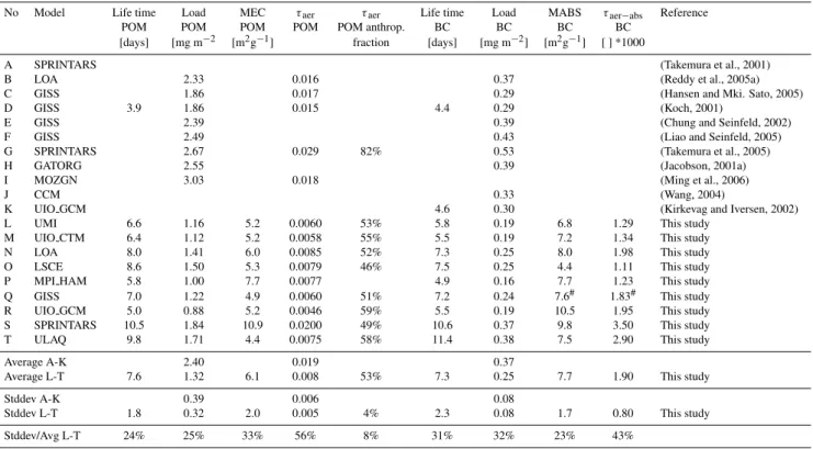
Table 3. Global mean values of load and optical properties of carbonaceous aerosol. All values correspond to the anthropogenic fraction. Life times are calculated from emission and load. POM: Particulate organic matter; BC: black carbon. MEC: dry mass extinction coefficient. Lines A-K: recently published model simulations; Lines L-T: Models used AeroCom emissions.
No Model Life time Load MEC τaer τaer Life time Load MABS τaer−abs Reference
POM POM POM POM POM anthrop. BC BC BC BC
[days] [mg m−2 [m2g−1] fraction [days] [mg m−2] [m2g−1] [ ] *1000
A SPRINTARS (Takemura et al., 2001)
B LOA 2.33 0.016 0.37 (Reddy et al., 2005a)
C GISS 1.86 0.017 0.29 (Hansen and Mki. Sato, 2005)
D GISS 3.9 1.86 0.015 4.4 0.29 (Koch, 2001)
E GISS 2.39 0.39 (Chung and Seinfeld, 2002)
F GISS 2.49 0.43 (Liao and Seinfeld, 2005)
G SPRINTARS 2.67 0.029 82% 0.53 (Takemura et al., 2005)
H GATORG 2.55 0.39 (Jacobson, 2001a)
I MOZGN 3.03 0.018 (Ming et al., 2006)
J CCM 0.33 (Wang, 2004)
K UIO GCM 4.6 0.30 (Kirkevag and Iversen, 2002)
L UMI 6.6 1.16 5.2 0.0060 53% 5.8 0.19 6.8 1.29 This study
M UIO CTM 6.4 1.12 5.2 0.0058 55% 5.5 0.19 7.2 1.34 This study
N LOA 8.0 1.41 6.0 0.0085 52% 7.3 0.25 8.0 1.98 This study
O LSCE 8.6 1.50 5.3 0.0079 46% 7.5 0.25 4.4 1.11 This study
P MPI HAM 5.8 1.00 7.7 0.0077 4.9 0.16 7.7 1.23 This study
Q GISS 7.0 1.22 4.9 0.0060 51% 7.2 0.24 7.6# 1.83# This study
R UIO GCM 5.0 0.88 5.2 0.0046 59% 5.5 0.19 10.5 1.95 This study
S SPRINTARS 10.5 1.84 10.9 0.0200 49% 10.6 0.37 9.8 3.50 This study
T ULAQ 9.8 1.71 4.4 0.0075 58% 11.4 0.38 7.5 2.90 This study
Average A-K 2.40 0.019 0.37
Average L-T 7.6 1.32 6.1 0.008 53% 7.3 0.25 7.7 1.90 This study
Stddev A-K 0.39 0.006 0.08
Stddev L-T 1.8 0.32 2.0 0.005 4% 2.3 0.08 1.7 0.80 This study
Stddev/Avg L-T 24% 25% 33% 56% 8% 31% 32% 23% 43%
# GISS absorption coefficient assumed to equal that of AeroCom models (7.7 m2g−1)
three source categories mentioned above should be treated as a total carbonaceous category, which we name hereafter (BCPOM).
The AeroCom model results are heterogeneous with re-spect to identifying carbonaceous aerosol categories, because the model structure with respect to the split of the carbona-ceous aerosols is difficult to change for just one experiment. To make the results from the different models more com-parable we chose to compute the missing values. This is done based on ratios established within those models having explicitly attributed RF to a category-split of the carbona-ceous particles. These ratios relate e.g. fossil-fuel BC-RF to total BC-RF (50%), fossil-fuel POM-RF to total POM-RF (25%). We assume linear additivity for biomass burning RF and fossil-fuel carbonaceous RF. The relations and the mod-els on which they are based are detailed in the footnotes of Table 4. The relations derived from global mean values as reported in Table 4 should not be seen as valid on a local level.
Carbonaceous aerosol life times, loads and optical proper-ties are found in Table 3. This table also reports AeroCom group results together with recently published data for com-parison. As for sulphate, the diversity in POM load and AOD is as large among AeroCom models as in the previous model
prediction result group. Results from AeroCom A and B sim-ulations are also similar. Comparing total POM AOD from our nine models shows slightly less POM AOD in B and de-spite equal emissions larger diversity in B (A: 0.018±44% versus B: 0.014±64%).
The variation in POM mass extinction coefficient is slightly more important (33%) as compared to that of POM lifetime (24%). The anthropogenic fraction of POM varies little (8%) but its variation indicates significant differences in removal patterns among models, given that the emissions were prescribed. However, the anthropogenic fraction of POM-AOD varies less than that of sulphate because, in con-trast, an additional process (chemical production) affects the fate of the natural and anthropogenic sulphur emissions. BC lifetime is smaller than that of POM in half of the Aero-Com models (L-P). Note that the biomass burning aerosol, with a higher fraction of POM, are emitted in the AeroCom emissions at higher altitudes than fossil fuel derived emis-sions and mostly in the dry season (Dentener et al., 2006). However, the mass absorption coefficient of BC also shows considerable variation. As Kinne et al. (2006) have shown, this variation can be explained in part by the variation in aerosol composition among the models. This is probably less important in our experiments B and PRE, because BC
Table 4. Anthropogenic aerosol forcing (RF) for different carbonaceous components: FFBC=fossil fuel black carbon, FFPOM= fossil fuel particulate organic matter, BB=biomass burning. “NRF POM”: normalized RF per unit POM optical depth; “NRF BC”: normalized RF per unit total absorption optical depth; Lines A-K: recently published; Lines L-T: Models used AeroCom emissions.
No Model NRF POM NRF BC RF RF RF RF RF RF Reference [Wm−2 [Wm−2 BCPOM POM BC FFPOM FFBC BB
τaer−1] τaer−abs−1 ] [Wm−2] [Wm−2] [Wm−2] [Wm−2] [Wm−2] [W m−2]
A SPRINTARS 0.12 –0.24 0.36 –0.05 0.15 –0.01 (Takemura et al., 2001) B LOA 0.30 –0.25 0.55 –0.02 0.19 0.14 (Reddy et al., 2005a) C GISS 0.35 –0.26 0.61 –0.13 0.49 0.065 (Hansen and Mki. Sato, 2005) D GISS 0.05 –0.30 0.35 –0.08$ 0.18$ –0.05$ (Koch, 2001)
E GISS 0.32 –0.18 0.50 –0.05$ 0.25$ 0.12$ (Chung and Seinfeld, 2002) F GISS 0.30 –0.23 0.53 –0.06$ 0.27$ 0.09$ (Liao and Seinfeld, 2005) G SPRINTARS 0.15 –0.27 0.42 –0.07$ 0.21$ 0.01$ (Takemura et al., 2005) H GATORG 0.47 –0.06 0.55 –0.01$ 0.27$ 0.22$ (Jacobson, 2001b) I MOZGN –0.34 –0.09$ (Ming et al., 2006)
J CCM 0.34 0.17$ (Wang, 2004)
K UIO GCM 0.19 0.10$ (Kirkevag and Iversen, 2002) L UMI –38 194 0.02 –0.23 0.25 –0.06$ 0.12$ -0.01 This study
M UIO CTM –28 164 0.02 –0.16$ 0.22$ –0.04 0.11 -0.05 This study N LOA –19 159 0.14 –0.16# 0.32# –0.04$ 0.16$ 0.02$ This study O LSCE –22 270 0.13 –0.17 0.30 –0.04$ 0.15$ 0.02$ This study P MPI HAM –14 165 0.09 –0.10# 0.20# –0.03$ 0.10$ 0.01 This study Q GISS –23 120 0.08 –0.14 0.22 –0.03$ 0.11$ 0.01$ This study R UIO GCM –13 184 0.24 –0.06 0.36 –0.02$ 0.18$ 0.08$ This study S SPRINTARS –5 91 0.22 –0.10 0.32 –0.01 0.13 0.06 This study T ULAQ –12 28 –0.01 –0.09 0.08 –0.02$ 0.04$ –0.03$ This study Average A-K 0.26 –0.24 0.44 –0.06 0.23 0.07
Average L-T –19 153 0.10 –0.14 0.25 –0.03 0.12 0.01 This study Stddev A-K 0.14 0.08 0.13 0.04 0.11 0.09
Stddev L-T 10 68 0.09 0.05 0.08 0.01 0.04 0.04 This study Stddev/Avg L-T 51% 45% 85% 38% 33% 47% 33% 323%
$ Models A–C are used to provide a split in sources derived from total POM and total BC; FFPOM=POM*0.25; FFBC=BC*.5; BB=(BCPOM)-(FFPOM+FFBC); BC=2*FFBC; POM=4*FFPOM
# Models L,O,Q-T are used to provide a split in components: POM=BCPOM*-1.16; BC=BCPOM*2.25
and POM loads are correlated through harmonized emission fields. With absent anthropogenic dust, no dust absorption will interfere in our diagnostics here. However, assump-tions on internal mixing and dependence of absorption on the presence of other aerosol components such as sulphate and aerosol water will create differences. Further investiga-tion of the underlying assumpinvestiga-tions in the different models is needed. We can suggest, that the optical properties of BC and POM are a source of considerable diversity among the AeroCom models with respect to RF calculations.
The corresponding RF values and forcing efficiencies are found in Table 4. The total BCPOM RF is positive (warming the Earth-Atmosphere System) for the AeroCom models and previous model predictions. As for sulphate, the BCPOM RF suggested by the AeroCom models is smaller in mag-nitude than that by non-AeroCom models (+0.10 instead of +0.26 Wm−2). This is consistent with smaller loads of both
BC and POM in the AeroCom simulations, which can partly be explained by using prescribed biomass burning emissions for the year 2000, which were relatively small compared to the average over the last decade (van der Werf et al., 2003). Also the fossil fuel inventory used in the AeroCom emis-sion data set referring to Bond et al. (2004) is low, especially over Europe. Emissions for total POM and BC in the origi-nal AeroCom A simulations were approximately 30% higher than those prescribed for AeroCom B (Textor et al., 2006; and Dentener et al., 2006). A comparison of the average POM AOD from the nine models analysed here also shows a drop of roughly 30% (POM AOD Exp. A: 0.0184; Exp. B: 0.0144). Note that the change in just the anthropogenic POM emissions can not be diagnosed due to missing information for AeroCom A.
The BCPOM RF estimates, and all other categories of car-bonaceous aerosol RF, vary considerably. In light of the large
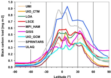
differences for aerosol absorption among AeroCom models this is not completely surprising. Aerosol absorption makes RF calculations dependent on environmental factors, result-ing in a less negative (or more positive) RF, especially when placed over highly reflective surfaces (e.g. snow, low clouds and even desert regions). In that context also spatial dif-ferences in burden distributions contribute (Fig. 1). Several models transport considerable amounts of BC towards the polar regions, while others are less diffusive or remove BC more efficiently close to emission sources (e.g. MPI HAM and UIO CTM). The diagnostics of long range transport is probably a good indicator of black carbon remaining at high altitudes, which in itself is a result of a less efficient washout process or an efficient vertical transport process parameteri-sation and differences in the treatment of black carbon age-ing. An evaluation of the BC fields with measurements is beyond the scope of this paper, and will be performed in fu-ture work for the AeroCom results.
A word of caution is needed before the individual source categories of carbonaceous aerosol RF are discussed: Since gaps in the submitted model results were filled by recom-puted values, the different estimates by source category (total BCPOM; total BC; total POM; fossil fuel BC: FFBC; fossil fuel POM: FFPOM and biomass burning: BB) are not com-pletely independent of each other. There is general agree-ment between AeroCom and non-AeroCom models that the POM-RF is negative and that BC-RF is positive – resulting overall in a slightly positive combined BCPOM RF (on an annual global basis). Comparisons between forcings asso-ciated to biomass burning and fossil fuel burning suggest a more positive (or less negative) fossil fuel RF, which is con-sistent with higher BC/POM ratios for fossil fuel emissions.
The inspection of the consistency of the BCPOM-RF with the split into either BC-RF+POM-RF or into FFBC-RF+FFPOM-RF+BB-RF reveals that the total carbonaceous aerosol RF is not always a linear combination of the two sorts of splits. This is partly due to the method used for filling gaps, where ratios established in other models are used. Sec-ondly it expresses the difficulty in ascribing a RF to indi-vidual carbonaceous aerosol source categories. The internal aerosol mixing and associated changes in forcing efficiency of especially black carbon but also POM is responsible for non-linear effects.
The diversity in component wise RF is largest for BB (323%). The component forcings of fossil fuel BC or POM and also those of total BC and POM vary between 33% and 47%. In absolute terms BB-RF shows similar varia-tion (±0.04 Wm−2) than the fossil fuel components (±0.01– 0.04 Wm−2). Variation in BCPOM RF (85%) is significantly larger than that of the sulphate RF. Altogether the carbona-ceous aerosol RF is responsible for an important part of the total RF diversity among models.
0.0 0.1 0.2 0.3 0.4 0.5 0.6 0.7 0.8 0.9 1.0 -90 -60 -30 0 30 60 90 Latitude [°] B la c k c a rb o n l o a d [ m g m -2 ] UMI UIO_CTM LOA LSCE MPI_HAM GISS UIO_GCM SPRINTARS ULAQ
Fig. 1. Zonal distribution of the atmospheric load of black carbon for the AEROCOM B (present-day emissions) simulation.
3.3 Total anthropogenic aerosol
All nine AeroCom models reported a component combined total aerosol RF based on the AeroCom emissions. Note again, that nitrate, ammonium and anthropogenic dust are not considered in AeroCom emissions. However, ammo-nium sulphate is implicitly assumed when deriving phate optical parameters (except for nucleation derived sul-phate in e.g. UIO GCM). The RF values can be found in Table 5 along with global annual averages for aerosol load (or mass) and aerosol optical depth (AOD) and fur-ther diagnostics of the aerosol RF. The anthropogenic AOD fraction (of only 25%±11% globally) leads to a negative all-sky RF of −0.22 Wm−2 and a cooling of the Earth-Atmosphere-System, that is an order of magnitude smaller than the warming attributed to the anthropogenic enhance-ment of green-house gas concentrations. Based on just these results, in the light of a low standard deviation of ±0.16 Wm−2, an overall warming by aerosol is unlikely. The non-AeroCom models show a similar RF and standard devia-tion of −0.20±0.21 Wm−2. However, additional uncertainty due to emissions and other forcing terms (such as the indi-rect forcing, nitrate and dust) need to be added to obtain the overall aerosol RF and its uncertainty.
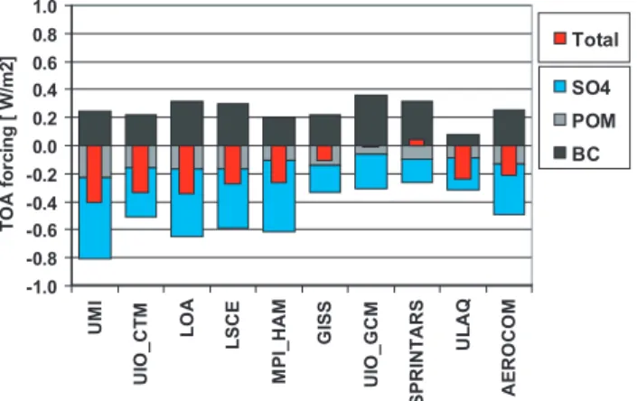
The relatively small cooling due to the direct aerosol RF is the result of warming of the BC containing components and opposite cooling by POM and sulphate, as illustrated in Fig. 2. An explanation for the relatively small standard devi-ation of the total aerosol RF is that the magnitude of negative (POM) and positive (BC) forcing is correlated. Their RF is correlated, because the residence times of the carbonaceous aerosol components in a given model are already connected. The correlation coefficient between BC and POM residence times from nine AeroCom models is 0.92.
Figure 3 shows the zonal distribution of the total aerosol RF in the nine AeroCom models. Most of the (negative) RF
Table 5. AeroCom (models H-P) and recent other model estimates (A-G) simulation results of anthropogenic aerosol load, anthropogenic aerosol optical depth (τaer), its fraction of present day total aerosol optical depth (τaerant hrop.), a dry mass extinction coefficient (MEC) as
well as cloud cover and clear-sky forcing efficiency per unit AOD. The all-sky total aerosol direct radiative forcing RF values are accompanied by the clear-sky and cloud-sky components together with their ratio. Solar surface forcing and solar atmospheric forcing are given for all-sky conditions.
No Model Load τaer τaer. MEC Cloud NRF RF RF top RF top RF top surface Atmospheric Reference [mg m−2] anthrop [m2g−1] cover clear-sky all-sky/ clear sky cloud-sky all-sky forcing forcing
fraction [Wm−2τaer−1] clear-sky [Wm−2] [W m−2] [Wm−2] all-sky [Wm−2] all-sky [Wm−2]
A GISS 5.0 79% +0.01$ –2.42$ 2.43$ (Liao and Seinfeld, 2005)
–0.39& –1.98& 1.59&
B LOA 6.0 0.049 34% 70% –0.53 –0.09 (Reddy and Boucher, 2004)
C SPRINTARS 4.8 0.044 50% 9.2 63% –18 0.08 –0.77 +0.36 –0.06 –1.92 1.86 (Takemura et al., 2005) D UIO GCM 2.7 0.021 6% 57% –17 0.83 –0.35 –0.25 –0.11 –0.60 –0.49 (Kirkevag and Iversen, 2002)
E GATORG 6.4 62% –0.89 –0.12 –2.5 2.38 (Jacobson, 2001a)
F GISS 6.7 0.049 –0.23 (Hansen et al., 2005)
G GISS 5.6 0.040 –0.63 (Koch, 2001)
H UMI 4.0 0.028 25% 7.0 63% –29 0.51 –0.80 –0.10 –0.41 –1.24 0.84 This study
I UIO CTM 3.0 0.026 19% 8.5 70% –33 0.40 –0.85 –0.07 –0.34 –0.95 0.61 This study
J LOA 5.3 0.046 28% 8.7 70% –18 0.44 –0.80 –0.16 –0.35 –1.49 1.14 This study
K LSCE 4.8 0.033 40% 6.9 62% –29 0.30 –0.94 0.08 –0.28 –0.93 0.66 This study
L MPI HAM 3.4 0.032 24% 9.6 62% –20 0.42 –0.64 0.00 –0.27 –0.98 0.71 This study
M GISS 2.8 0.014 11% 5.0 57% –21 0.36 -0.29 0.05 –0.11 –0.81 0.79 This study
N UIO GCM 2.8 0.017 11% 6.2 57% –0.01 –0.84 0.84 This study
O SPRINTARS 3.2 0.036 44% 11.1 62% –10 –0.12 –0.35 0.34 +0.04 –0.91 0.96 This study
P ULAQ 3.7 0.030 23% 8.1 –26 –0.79 –0.24 This study
Average A-G 5.3 0.041 66% –0.64 –0.20 –1.88 1.55
Average H-P 3.7 0.029 25% 7.9 63% –23 0.33 –0.68 0.02 –0.22 –1.02 0.82
Stddev A-G 1.3 0.012 9% 0.24 0.21 0.76 1.20
Stddev H-P 0.9 0.010 11% 1.8 5% 7 0.21 0.24 0.16 0.16 0.23 0.17
Stddev/Avg H-P 24% 33% 45% 23% 8% 32% 63% 35% >100% 72% 23% 21%
& External mixture
$Internal mixture
is located between 20 and 60◦N and forcing differences are largest especially at northern mid-latitudes. The highest pos-itive forcings in the northern high latitudes by the GISS and the UIO GCM models coincide with their relatively high BC loads there. Among all AeroCom models only SPRINTARS suggests a very weak positive total RF, which can be traced back to a relatively small negative sulphate RF and the largest positive cloud sky forcing. This high cloud sky forcing is also found in another SPRINTARS simulation (model C) (Take-mura et al., 2005).
The diversity of the all-sky RF among AeroCom models is as large as 73%. This is considerably larger than the di-versity in load (24%), AOD (33%), absorption optical depth (43%) and clear-sky RF (35%). The reasons for the differ-ences in RF among the AeroCom models are the subject of discussion in the following sections. Based on the additional output provided by the AeroCom models, individual steps from emissions to forcing can be diagnosed.
The AeroCom diagnostics include two more parameters that concern changes of the radiation balance due to aerosol present in the atmosphere: “Atmospheric forcing” which ac-counts for solar absorption of incoming radiation in the at-mospheric column – and “surface forcing” which reflects the incoming solar radiation at surface level, which is counter-balanced by other heat fluxes at surface level and is thus im-portant for the hydrological cycle but which is not a good indicator of climate warming. The surface forcing equals the
ToA-RF minus the atmospheric forcing. These are rarely re-ported in other publications and shall be mentioned here, be-cause they constitute an important element for the regional climate impact of the aerosol. The solar all-sky atmospheric forcing attains a global average of +0.82 Wm−2and conse-quently the solar surface forcing is at −1.02 Wm−2. The at-mospheric forcing is considerably larger than the ToA-RF for all models. The absolute value of the diversity for the atmospheric forcing is comparable to that of RF. The rela-tive standard deviation is only 21%. An inspection of the individual model values of RF and atmospheric forcing re-veals that the two parameters are not correlated. Since at-mospheric forcing reflects absorption of shortwave radiation we have also tested correlation with the three major compo-nents using the average model values from the Tables 2, 4 and 5. The highest correlation coefficient is found for BC-RF (r=0.54), while correlation with POM-BC-RF (r=0.05) and SO4-RF (r=0.02) is absent. Measurements of the radiation budget changes throughout the column can thus be helpful to better understand the carbonaceous RF component. The In-dian Ocean Experiment (INDOEX, Ramanathan et al., 2001 and references therein) showed the importance of absorption by aerosol in the atmospheric column. Their observations show that the local surface forcing (−23 Wm−2) was signifi-cantly stronger than the local RF at the top of the atmosphere (−7 Wm−2).
-1.0 -0.8 -0.6 -0.4 -0.2 0.0 0.2 0.4 0.6 0.8 1.0 U M I U IO _ C T M L O A L S C E MP I_ H A M G IS S U IO _ G C M SPR IN T A R S U L A Q A E R O C O M T O A f o rc in g [ W /m 2 ] SO4 POM BC Total
Fig. 2. Direct aerosol forcing for the three major anthropogenic aerosol components sulphate, black carbon and particulate organic matter in the AeroCom models. Shown on top in red is also the total direct aerosol forcing as diagnosed from a full aerosol run.
3.4 Analysis of all-sky, clear-sky and cloud-sky forcing dif-ferences
The all-sky solar RF, which was discussed in the previous section, is in addition to parameters that influence clear-sky forcing also modulated by clouds. The clear-sky aerosol RF is influenced by aerosol properties (mainly amount and ab-sorption), by the solar surface albedo and the distribution of water vapor. The presence of cloud changes the radiation field dramatically and can change the sign of aerosol RF. All-sky RF is consequently not just a cloud cover area-weighted clear-sky RF. Therefore we compare here the simulated an-nual global fields for all-sky (RF) and clear-sky ToA forcing (RFcs) and cloud-sky ToA forcing (RFcl) from the AeroCom simulations as summarized in Table 5. The cloud-sky forcing was not reported by modelers and is recomputed here based on global annual fields of RF, RFcsand individual model de-rived information on cloud cover (C):
RFcl= RF/C − (1 − C)/C∗RFcs. (1) Clear-sky RF fields of most of the different AeroCom mod-els in Fig. 4 display similar patterns. Negative forcings are predicted above industrialized zones of the Northern Hemi-sphere and over tropical biomass burning regions. Positive, or less negative, forcings are simulated over bright desert surfaces and over snow-cover. Larger differences among models over desert regions indicate differences in desert so-lar albedo assumptions for which we have unfortunately in-complete documentation. The diversity of clear sky-forcing (35%) in Table 5 is found to be smaller than that of the all-sky RF (73%), which reflects better understanding of clear-sky radiative effects.
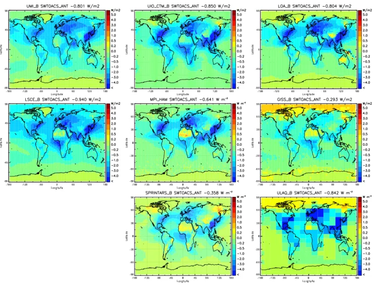
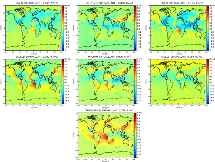
All-sky (aerosol) annual RF fields of the different Aero-Com models in Fig. 5 indicate that the all-sky aerosol RF is almost everywhere less negative than clear-sky forcing
-1.5 -1.0 -0.5 0.0 0.5 1.0 -90 -60 -30 0 30 60 90 Latitude [°] R F [ W m -2 ] UMI UIO_CTM LOA LSCE MPI_HAM GISS UIO_GCM SPRINTARS ULAQ
Fig. 3. Zonal distribution of the total direct aerosol forcing for all-skies.
(Fig. 4). Under all-sky conditions, the clear-sky forcing val-ues apply only to cloud-free regions (ca. 30%), while in con-junction with clouds, aerosol (solar) RF is modulated de-pending among other parameters on the relative position of aerosol and clouds. If clouds are optically thick and aerosol is below cloud, solar radiation is reflected to a large part back to space, before it can interact with aerosol. RF forcing by aerosol can then be ignored. If aerosol is above clouds, how-ever, the high solar reflectivity of clouds will cause a pos-itive aerosol RF, as observed over surfaces with large solar albedos (e.g. desert, snow). Absorbing aerosol reduces so-lar reflection to space, which translates into a positive ToA forcing.
We find that the cloud-sky aerosol ToA forcing is a use-ful diagnostic tool. Cloud-sky annual ToA forcing fields of the different AeroCom models in Fig. 6 display characteris-tic spatial features, which differ from model to model, and can be linked to physical explanations as found below. The diversity of cloud-sky forcing attains >100%, due to the un-certainty in sign of this forcing term. The variation in abso-lute terms, taken into account the large cloudy area fraction, of ±0.16 Wm−2is at least as important as that of the clear-sky forcing ±0.24 Wm−2 (see Table 5). Globally averaged cloud-sky forcings vary between +0.34 and −0.16 Wm−2 and for almost all models deviate significantly from zero. Since the cloud-covered area is 70%, it dominates over clear-sky conditions, and small differences of cloud-clear-sky ToA forc-ing are an important explanation for the all-sky ToA forcforc-ing diversity among the AeroCom models. Global annual aver-ages of RF, RFcsand RFclare put together in Fig. 7.
Why are models showing positive and negative cloud-sky forcings? An interesting comparison can be made for the LOA and the LSCE model. While the underlying GCM and thus meteorology and transport and emissions are the same, the aerosol dynamics, removal, optical properties and forcing calculations are not. The absolute difference in cloud cover is a result of different diagnostics provided to the AeroCom database. The relative cloud cover distribution is very much
Fig. 4. Maps of the total direct aerosol forcing in clear-sky conditions in the AeroCom models.
alike. We diagnose a negative cloud forcing for LOA and a slightly positive one for LSCE. Clear sky forcing in the LSCE is 20% more negative. Figure 5 shows similar positive forcing in LOA and LSCE in large regions where absorbing anthropogenic aerosols above marine stratocumulus clouds are responsible for positive cloud-sky forcing. The global av-erage becomes negative for LOA because important negative cloud forcing contributions are diagnosed for North America, Europe and South East Asia. LOA also shows more negative sulphate forcing than LSCE. Higher sulphate AOD in LOA (sulphate AOD LOA:0.35; LSCE: 0.23) can result in more scattering when thin clouds are present and thus produce a negative overall cloud-sky forcing (Zhou et al., 2005).
Looking at all models we find that the three models with the largest negative aerosol all-sky RF also have negative cloud-sky forcings (UIO CTM, UMI, LOA). Models with low BC loads (UIO CTM, UMI) do not show positive all-sky forcing in any region. Elevated biomass burning aerosol seems to be responsible for positive cloud-sky forcing over the Atlantic off South Africa. UIO CTM simulates such
pos-itive cloud-sky forcing only in the North American and South East Asian polluted areas. While UIO CTM has a negative cloud sky RF for the annual mean the cloud-sky RF in the biomass burning season (July–September) is positive.
Positive cloud-sky forcings are responsible for the less negative all-sky forcing in LSCE, GISS and SPRINTARS. Note that the model with the largest cloud-sky forcing (SPRINTARS) also simulates the second largest BC loads. MPI HAM shows similar cloud-sky forcing over the ocean as LOA and LSCE, but simulates important positive con-tributions also over industrialised mid-latitude regions and above desert areas. This indicates a higher sensitivity of the RF to the albedo – either from bright desert surfaces or clouds. The GISS model shows a small negative all-sky forc-ing as a combination of the lowest sulphate load and RF and positive cloud-sky forcing in the northern hemisphere, es-pecially over South East Asia and the Pacific. Low all-sky forcing for the UIO GCM models can in part be explained by low sulphate AOD and high BC absorption.
Fig. 5. Same as Fig. 4 but all-sky condition total direct aerosol forcing in the AeroCom models. The ULAQ all-sky forcing is constructed from computed clear-sky forcing, assuming no cloud sky forcing and 70% cloud cover.
3.5 Sensitivity analysis of major factors linking emission and forcing
Having used identical emissions and analysed meteorology for the same year offers the chance to analyse the differ-ent steps from emission to forcing with small interference from large spatial differences in emission and aerosol fields. Few major factors are investigated here for their impact on resulting aerosol forcing diversity among AeroCom models. We neglect to analyse the specific impact on RF of the dif-ferent environments in the models due to difdif-ferent humidity fields and surface albedo, mainly because we have insuffi-cient diagnostics available. A simplified diagnostic model equation assumes that the RF is a product of emission flux (E), residence time (or life-time) (t), mass extinction effi-ciency (mass to AOD conversion) (mec) and the radiative forcing efficiency (NRF) with respect to AOD:
RF = E ∗ t ∗ mec ∗ NRF. (2)
Since the emissions E are equal, any variability of the three remaining factors (t, mec, and NRF) influences the simulated forcing. While this is valid for POM, factors of relevance were chosen differently for sulphate, BC and total aerosol. For the total aerosol we introduce the forcing efficiency for clear-sky RF and the ratio of all-sky RF over clear-sky RF as factors. BC RF is related to absorption AOD and a forcing ef-ficiency per unit absorption AOD. Sulphate forcing depends also on the chemical production of aerosol sulphate.
Data from Tables 2, 3, 4 and 5 provide individual resi-dence time, mass extinction coefficient and forcing efficien-cies for sulphate, BC and POM and total aerosol. Then for each model n, factor x and species i the hypothetical RFx,n,i (for the case that only the factor x was a source of variabil-ity) is defined by RFx,n,i=xn/<x>∗RFi, where xnis the fac-tor value for model n, <x> is the AeroCom mean for the factor and RFi is the mean AeroCom forcing for the aerosol species i.
Fig. 6. Same as Fig. 4 but cloud-sky condition total direct aerosol forcing in the AeroCom models.
All RFx,n,i are presented for each model and factor in Fig. 8 separately for the four species: sulphate, BC, POM and total aerosol. In addition, the original model derived RF values are shown in the last column. Model specific lines connect estimated RFx,n,i mainly for readability pur-poses. Cross-overs indicate compensating effects, which re-duce model diversity for the “final” aerosol RF estimate.
The sensitivity for the total anthropogenic forcing in Fig. 8a shows that the clear-sky forcing efficiency and the all-sky forcing calculation themselves are responsible for large diversity among the AeroCom models. However, it is prob-ably not so much the radiative transfer calculation method, but differences in composition and most of all the represen-tation of clouds that contribute to the diversity. In compari-son, residence time and mass extinction efficiency introduce a relatively small diversity on total RF estimates. Numer-ous cross-overs indicate that each model has its own way of translating emission into forcing.
The sensitivity of BC forcing in Fig. 8b is discussed as a function of the aerosol absorption coefficient. The absorp-tion coefficient based on the global values of absorpabsorp-tion and
load in Table 3 ranges from ∼4.5 (UMI and LSCE) up to ∼10 (SPRINTARS and UIO GCM). Note that this is derived from the ratio of anthropogenic absorption and the BC load. It does thus include effects of internal mixing of BC with other species and eventually from absorption by POM. In contrast to the sensitivity of the total aerosol RF, BC res-idence time and BC absorption efficiency cause significant scatter in BC-RF. However, the forcing efficiency remains the major source of diversity. Inspecting the cross-overs of the modelled pathway from emission to forcing reveals much more diverse pathways from emission to BB-RF than those for total aerosol RF.
The sensitivity analysis for POM-RF and sulphate-RF are presented in Figs. 8c and d, respectively. Sulphate residence times together with chemical production constitute a major source of diversity, because formation of sulphate involves additional processes, such as SO2 deposition and chemical production in gas and cloud phase. Interestingly small sul-phate residence times (or fast removal) are compensated con-siderably by high sulphate dry mass extinction coefficients for SPRINTARS, ULAQ, MPI HAM and UIO CTM, and
vice versa for GISS, LSCE and LOA. Since hygroscopic growth is a major factor in enhancing sulphate aerosol ex-tinction one might speculate that larger residence times result from sulphate transported into dry upper air tropospheric lay-ers. This would coincide with little hygroscopic growth and thus would diminish the global extinction coefficient. In-spection of the AeroCom database shows that indeed LOA and LSCE have roughly four times as much sulphate burden located in the upper troposphere (>5 km) than models like SPRINTARS and UIO CTM. Diagnosing the vertical distri-bution of the anthropogenic aerosol water and humidity fields is suggested for future work to give more clarity for this be-haviour of the models. Total aerosol water as diagnosed in AeroCom A is dependent on global sea salt loads and is an insufficient diagnostic here.
Different forcing efficiencies for sulphate further seem to complicate the pathway towards forcing. Models with rel-atively high forcing efficiencies based on sulphate optical thickness are GISS and UMI. Altogether we have to stress that among the four factors influencing the sulphur forcing estimate, none can be called the single major cause of diver-sity.
POM residence times and extinction coefficients are mi-nor sources of variation. With the exception of SPRINTARS the variation in POM mass extinction coefficient is small. This does not mean that the POM mass extinction coefficient is known well, rather that the models use similar assump-tions. A plausible hypothesis is that the models applied the same size distribution as suggested by the AeroCom emis-sion dataset description and that little humidity growth is as-sumed for the organic particle fraction. For POM we find that the forcing efficiency gives rise to even larger diversity than found in the original forcing estimates in the model output. Due to the lack of diagnostics we cannot verify here all the assumptions made for the POM forcing efficiencies. Internal and external mixing assumptions and absorption properties of the POM may not be as clearly split from the BC as would be needed to clearly understand the diversity in POM forcing efficiency.
4 Summary and conclusions
As a summary annual fields averaged from all regridded AeroCom model results are presented in Fig. 9 for anthro-pogenic aerosol optical depth, the associated RF, the local standard deviation of RF from the nine AeroCom models, solar atmospheric forcing and surface forcing as well as the clear-sky RF.
Anthropogenic aerosol optical depth shows distinct max-ima in industrialised regions and above tropical biomass burning regions (Fig. 9a). The prevailing location of the an-thropogenic aerosol is over continents. On average anthro-pogenic aerosol optical depth makes up only 25% of the to-tal aerosol optical thickness. These two characteristics keep
-1.0 -0.8 -0.6 -0.4 -0.2 0.0 0.2 0.4 0.6 0.8 1.0 U M I U IO _ C T M L O A L S C E MP I_ H A M G IS S U IO _ G C M SPR IN T A R S U L A Q A E R O C O M T O A fo rc in g [ W m -2 ] Cloudy sky Clear sky Total
Fig. 7. Total direct aerosol forcing, and contributions from clear-sky and cloud-clear-sky conditions. For the latter clear clear-sky and cloud-clear-sky area fractions in each grid box are multiplied with the clear sky and cloud-sky forcing values, so that they add up to the total area weighted all-sky RF.
any comparison with satellite derived aerosol effects a chal-lenging task, since the satellite observations are more reliable over the ocean. Furthermore Fig. 9e shows that the more readily observable clear-sky forcing is dominantly linked to high anthropogenic AOD over the continents. Table 6 com-pares our work to the recent compilation of observational based RF estimates by Yu et al. (2006), separating AOD, RF and forcing efficiency values between land and ocean. The comparison is also contained to the band between 60◦S and 60◦N, where satellite observations are abundant and reliable throughout the year. Both AOD and forcing efficiency are lower in the AeroCom models, and consequently the RF is almost twice in the observational based RF. AOD differences in clear sky over the ocean could be attributed to missing anthropogenic aerosol in the models (nitrate, dust, underesti-mated emission sources), but also any other systematic error in handling the aerosol cycle up to the aerosol optical prop-erties. An overestimation of the anthropogenic fraction of AOD and undetected cloud contamination may be the cause for high satellite retrievals. However, the large difference in clear-sky forcing efficiency over the ocean points to impor-tant differences in the clear-sky forcing calculation itself, a problem which is thought to be less difficult to solve than RF over land and in cloud conditions. The more negative forcing based on observational studies driven by satellite retrievals is confirmed by work e.g. from Bellouin et al. (2005) and Kauf-man et al. (2005) (RF over ocean −0.8 Wm2and −1.4 Wm2). As long as these differences are not solved we may assume from this comparison, that the model based RF estimate is a low estimate.
The aerosol RF attains −0.22 Wm−2, suggesting in the long term a small impact through aerosol induced climate change on global surface temperature from the presence of anthropogenic aerosol in the atmosphere. General

![[PDF] Introduction à HTML 5 ressource de formation approfondie | Cours INFORMATIQUE](data:image/gif;base64,R0lGODlhAQABAIAAAP///wAAACH5BAEAAAAALAAAAAABAAEAAAICRAEAOw==)