Secondary fast reconnecting instability in the sawtooth crash.

HAL Id: hal-01780899

https://hal.archives-ouvertes.fr/hal-01780899

Submitted on 16 May 2018

HAL is a multi-disciplinary open access archive for the deposit and dissemination of sci-entific research documents, whether they are pub-lished or not. The documents may come from teaching and research institutions in France or abroad, or from public or private research centers.

L’archive ouverte pluridisciplinaire HAL, est destinée au dépôt et à la diffusion de documents scientifiques de niveau recherche, publiés ou non, émanant des établissements d’enseignement et de recherche français ou étrangers, des laboratoires publics ou privés.

Secondary fast reconnecting instability in the sawtooth

crash.

Daniele del Sarto, Maurizio Ottaviani

To cite this version:

Daniele del Sarto, Maurizio Ottaviani. Secondary fast reconnecting instability in the sawtooth crash.. Physics of Plasmas, American Institute of Physics, 2017, 24, pp.12102 - 12102. �10.1063/1.4973328�. �hal-01780899�

D. Del Sarto and M. Ottaviani

Citation: Phys. Plasmas 24, 012102 (2017); doi: 10.1063/1.4973328

View online: http://dx.doi.org/10.1063/1.4973328

View Table of Contents: http://aip.scitation.org/toc/php/24/1

Secondary fast reconnecting instability in the sawtooth crash

1

Institut Jean Lamour, UMR 7198 CNRS – Universit!e de Lorraine, F-54506 Vandoeuvre-l!es-Nancy, France

2

CEA, IRFM, F-13108 Saint-Paul-lez-Durance, France

(Received 9 March 2016; accepted 14 December 2016; published online 3 January 2017)

In this work, we consider magnetic reconnection in thin current sheets with both resistive and electron inertia effects. When the current sheet is produced by a primary instability of the internal kink type, the analysis of secondary instabilities indicates that reconnection proceeds on a time scale much shorter than the primary instability characteristic time. In the case of a sawtooth crash, non-collisional physics becomes important above a value of the Lundquist number, which scales likeS! ðR=deÞ12=5, in terms of the tokamak major radiusR and of the electron skin depth de. This value is commonly achieved in present day devices. As collisionality is further reduced, the charac-teristic rate increases, approaching Alfv!enic values when the primary instability approaches the collisionless regime.Published by AIP Publishing. [http://dx.doi.org/10.1063/1.4973328]

I. INTRODUCTION

Current sheets are a common occurrence in laboratory and space plasmas. They appear as a local two-dimensional current concentration and they can be either the natural prod-uct of convective, often turbulent, plasma motion, or the result of a plasma instability entering its non-linear stage.

In this work, we study the instability of generic current sheets, addressing the question of whether reconnection can be fast enough to account for the observed rates of common events such as the sawtooth crash in a tokamak and possibly solar flares.

We consider a plasma characterized by a non-uniform average magnetic fieldB0, varying on a characteristic scale lengthL0. The structure of a current sheet is an almost planar current concentration of extension L in two spatial dimen-sions and thicknessa_{$ L. Note that we keep L and L}0 dis-tinct although often in the literature L_{! L}0 or it is even

assumed thatL_{¼ L}0. By definition, the current density in the sheet would differ appreciably from the ambient current den-sity. However one can argue, and it will be shown below, that such current concentration is unstable to fast growing perturbations. Therefore, the current density in the sheetJcs cannot exceed too much the ambient current densityJ0, and therefore, one can reasonably assumeJcs! J0! B0=L0.

Moreover, a current sheet would generally evolve in time. However, when studying its stability, it is convenient to assume it to be in a quasi-stationary state, if one is inter-ested in instability growth rates much faster than the underly-ing evolution rate. As a consequence, a current sheet can be modeled as a planar system in local force balance. In the fol-lowing, we further assume that the ambient magnetic field is almost constant and that the current density in the sheet is almost aligned to it.

The current in the sheet produces a magnetic field Bcs! Jcsa, which lays in the plane and it is transverse to the

main magnetic field. From the previous estimate ofJcs, one concludes

Bcs! B0

a L0

: (1)

This scaling is certainly pertinent when the current sheet is the result of a largeD0_{primary instability as in the case of}

the sawtooth phenomenon, which is discussed in detail in Sec. III. In this instance, scaling(1) marks the transition to the nonlinear phase ifa is the linear layer width. Therefore, in this context, we are assuming that the current sheet becomes unstable to a secondary instability at an early stage of the nonlinear evolution of the primary instability, a result we will find consistent with the estimates derived later in this work. Our logic will be outlined in a greater detail at the end of Sec.II.

Note also that, by assuming this scaling ofBcswith the current sheet thickness, we depart fundamentally from previ-ous works,1–11 where the scaling Bcs! B0 is implicitly

assumed. The implications of this different assumption are discussed more in detail in Sec.IV. Here, we anticipate that Pucci and Velli6 pointed out that by increasing the current sheet aspect ratio tearing mode theory predicts an increasing growth rate, reaching the Alfv!enic limit at a characteristic aspect ratio that depends on the regime considered.6–11 The dependence of the growth rate on the aspect ratio is exploited in an essential way also in the present work, as discussed later.

Moreover, the presence of a strong guide fieldB0allows one to treat the problem in the framework of reduced MHD. In this respect, we depart from the work of Ref. 12, where the guide field is assumed zero.

In the following, we consider the resistive case, described by the model

1 c2 A @tr2_?/ þ ^u ' $r^ 2_?/^ ! " ¼ rjjJ^jj; (2) @tw þ ^u ' $^w ¼ (^g ^^ J_jj; (3) a)

Electronic mail: daniele.del-sarto@univ-lorraine.fr b)_{Electronic mail: Maurizio.Ottaviani@cea.fr}

1070-664X/2017/24(1)/012102/11/$30.00 24, 012102-1 Published by AIP Publishing.

written in terms of the normalized stream function ^

/ ) c/=B0, where/ is the electrostatic potential, and of the

normalized magnetic flux function ^_{w ) w=B}0. Here, the

cur-rent is given by ^J_{jj) (r}2

?w, the velocity is ^u ¼ b^ 0* $^/,

and the magnetic field is ^B_{¼ b}0( b0* $^w, with b0, the

unit vector of the local ambient magnetic fieldB0. Moreover,

we have introduced the Alfv!en velocity c2

A) B20=ð4pmin0Þ

and the magnetic diffusivity ^_{g ) c}2_{g=ð4pÞ. The symbol jj}

refers to the parallel component with respect to the total magnetic field, and_{? refers to the components perpendicular} to the local ambient field. Their exact expression depends on the context and they will be later specified in the case of slab and cylindrical geometry. Note that in Eqs. (2) and (3), lengths and times still appear in dimensional units.

In the following, we first derive the scaling of fast recon-nection in a general large aspect ratio slab (Sec. II). Then, we apply the result to the sawtooth problem, by evaluating whether the sawtooth crash can result from the instability of the current sheet generated by a primary m_{¼ 1 mode in a} cylindrical tokamak (Sec.III). In particular, we compare our conclusions with the existing numerical results (Sec. III B), and we analyze the transition to the non-collisional regime. We finally point out the difference with other works on fast reconnection, and we outline possible future work (Sec.IV). The complementary material is given in the appendixes, with brief reviews of the notion of “fast” in reconnection literature (Appendix A), of numerical results and experimental obser-vation of secondary reconnection (Appendix B), and of the asymptotic matching technique for stability calculations (Appendix C).

Before proceeding with Sec. II, we must point out that all the following calculations and results must be considered as an asymptotic analysis in terms of dimensionless parame-ters such as the normalized resistivity or its inverse (the Lundquist number), which will be considered arbitrary small (large) and the normalized electron skin depth. All quantities not depending on these parameters, such as certain geometri-cal factors like the tokamak aspect ratio, are assumed of order unity. Quantities of order unity will not be carried along in the calculations. Moreover, if a certain process occurs on a longer time scale (in the asymptotic sense) than another one, it will be considered as stationary for the pur-pose of computing the dominant behavior of the second one. Likewise, if a process has a characteristic length which is much smaller, in the asymptotic sense, than the scale length of the structure in which it is developed, it is reasonable to carry out a local analysis within a simplified geometry, much like what one would do in WKB theory.

Finally, we draw the attention of the reader to the fact that the secondary reconnecting instability we refer to in this paper is a standard tearing-type instability whose asymptotic scaling results to be compatible with experimentally observed disruptions in tokamaks because of geometrical rescaling arguments related to the current sheet aspect ratio: it is thus “fast” enough to possibly account for measurements but it is not necessarily Alfv!enic, although we will show that its growth rate can attain the ideal regime as electron-inertia effects are taken into account. We refer the reader to Appendixes AandBfor a summary on different examples of

fast and nonlinear reconnection models frequently encoun-tered in the literature.

II. SCALING OF THE MAXIMUM RECONNECTION RATE

Labeling with “eq” the equilibrium quantities and leav-ing the perturbations unlabeled, we start by linearizleav-ing Eqs. (2)and(3)around an equilibrium with ^/eq¼ 0 (no flow)

1 c2 A @tr2_?/ ¼ r^ keqJ^kþ rkJ^keq; (4) @tw þ r^ keq/ ¼ (^g ^^ Jjj; (5) where_{rk¼ ^}B_{' $.}

Adopting a local Cartesian coordinate system, we indi-cate with x the coordinate perpendicular to the sheet, y the direction of the transverse magnetic fieldBcs, andz the direc-tion of the ambient fieldB0. Moreover, for the sake of simplic-ity, one can assume a symmetric current distribution, such that Bcs¼ 0 at x ¼ 0 and two dimensional perturbations such that @z¼ 0.

Using(1), in the neighborhood ofx¼ 0, the parallel gra-dient operator takes the form

rjjeq! B0 csð Þ0 B0 # $ kx_! kx L0 # $ : (6)

The stability analysis of Eqs.(4)and(5)can be carried out with an asymptotic matching technique. A review of this known technique is given inAppendix C. In the following, instead, we directly work out the scaling of the growth ratec and of the inner reconnecting layer widthd in both the tear-ing (labeled as “T”) and internal kink (labeled as “K”) regimes. We recall that these regimes are identified by the conditions D0d < 1 and D0d > 1, respectively, where D0 is the usual tearing mode stability parameter.13The scaling can be obtained, up to numerical constants, without carrying out the detailed asymptotic matching calculations, by taking x_{! d, so that rjjeq! ðkd=L}0Þ. Moreover, using the fact that

k$ d(1; @x! d(1 and the estimate ^/00 ! ^/=d2, we obtain

the following heuristic balance relations, respectively, from Eq.(4)(l.h.s. and first r.h.s. term) and from Eq.(5)

1 c2 A c d2/ !^ kd L0 @2 xw;^ c^w ! kd L0 ^ / ! ^g@2 xw:^ (7)

These can be now specialized by estimating the per-turbed current density respectively as @2

xw ! ^w=d^ 2K for the

internal-kink (large-D0regime) and as@2

xw ! ^wD^ 0=dTfor the

tearing mode (small-D0, constant-w regime).

Introducing the macroscopic Alfv!en time s0 ) L0=cA

and the Lundquist number referred to the macroscopic scales S0) L0cA=^g, the following scalings are obtained:

cTs0! S( 3 5 0 ðkL0Þ 2 5 D0_L 0 ð Þ45_{; (8)} dT L0! S (2 5 0 ðkL0Þ( 2 5 D0_L 0 ð Þ15_{; (9)}

cKs0! S( 1 3 0 ðkL0Þ 2 3_{; (10)} dK L0 ! S (1 3 0 ðkL0Þ( 1 3_{: (11)}

Note that these scalings do not depend explicitly on the current sheet thickness a. However, in the tearing regime, they do depend implicitly ona via D0, which also brings in an additional dependence on the wavenumber. If the aspect ratioL/a is sufficiently large so that many wave-numbers are excited, a fastest growing mode exists13–16at the wavenum-berkMðS0Þ corresponding to the transition between the

tear-ing and the internal kink regimes. This transition occurs whenD0d ’ 1.

In order to see this, one has to specify the dependence of D0_{ona and k. Here, we adopt the expression obtained for the}

Harris17 pinch for small ka, that is, well above the tearing instability threshold

D0_! 1

ka2: (12)

Note that the dependence_{!1=k of D}0for smallk is fairly common and that, in any case, what follows can be easily generalized to a different10power-law dependence.

Using Eq.(12)in Eqs.(9)and(11), we obtain

kML0! S( 1 4 0 L0 a # $3 2 ; (13) cMs0! S( 1 2 0 L0 a # $ ; (14) dM L0 ! S (1 4 0 L0 a # $(1 2 : (15)

As indicated in the Introduction, the above results are of practical interest only if the underlying dynamics occurs at a rate lower than the estimate(14).

When the current sheet is the result of a large-D0primary instability of a quiescent plasma, the time scale of its dynam-ics can be obtained from(10)by takingk_{! L}(1

0 . This gives

cIs0 ! S(1=30 . The corresponding layer width is an estimate

of the current sheet width, a! dI ! L0S(1=30 . Moreover, as

the system enters the nonlinear phase, the current density in the sheet is of the order of the equilibrium one and its mag-netic field can be estimated as in Eq.(1). Henceforth, a full description of the magnetic structure would require a non-linear treatment of the type carried out in Refs. 24and25. However, in the following, it is enough to assume that a cur-rent sheet centered on the (primary) X-point is produced, without further details on the precise form of the nonlinear structure. The existence of such a current sheet is indeed shown in Refs.24and25, and observed in several numerical studies. In order to analyze the instabilities of such a struc-ture, we further conjecture that in this early nonlinear phase the current sheet width still scales like the linear layer width of the primary instability. Any other hypothesis would require additional explanation. Finally, we assume that the (primary) nonlinear structure produced at the end of the

primary instability phase evolves sufficiently slowly that it can be considered as stationary for the purpose of evaluating the secondary instability growth rate, a condition that can be verifieda posteriori. As a reference evolution rate of this pri-mary nonlinear structure, we can assume the linear growth rate of the primary instability. If anything, the evolution rate of the nonlinear structure issued from a resistive instability is usually found slower.

Using this information, one can estimate the maximum growth rate of the secondary instability from(14)

cMs0! S(

1 6

0 ; (16)

which is clearly higher than the primary instability growth rate. One concludes that the current sheet produced when a high D0 _{primary instability enters the nonlinear phase}

becomes quickly unstable, as soon as the primary current sheet becomes sufficiently thin. An application of this mech-anism to the sawtooth crash will be given in Sec.III.

More generally, current sheets occur as magnetic flux tubes are stretched and twisted by plasma advection. In an ideal plasma, this mechanism produces thinner and thinner current sheets. In a turbulent plasma with comparable kinetic and magnetic energy, the characteristic time is the Alfv!en time s0. Therefore, a current sheet will break up when its instability rate exceeds s(1

0 . From (14), one then deduces

that the current sheet thickness must be of the order of a

L0! S (1

2

0 : (17)

Note that forL0! L this scaling is the same as the

com-monly quoted Sweet-Parker thickness. However, the analogy appears only superficial. This thickness has been obtained here as the necessary condition for the break-up of a sheet formed by Alfv!enic motion rather than as the result of a steady reconnection process. Eq. (17) also represents the modified threshold aspect ratio for the trigger to the resistive “ideal” tearing mode in the quasi-ideal limit, as it is meant in Refs.6and10, once the Alfv!en time referred to the cur-rent sheet,scs, is rescaled to the macroscopic one according toscs¼ ðaB0Þ=ðL0BcsÞs0, while assuming(1).

III. SECONDARY FAST RECONNECTION AT THE TOKAMAK n5m51 RESONANT SURFACE

We now apply the above results to them_{¼ n ¼ 1 internal} kink (IK) instability in a large aspect ratio tokamak. The IK instability is considered an element of the sawtooth cycle,18an almost periodic oscillation of plasma temperature character-ized by a slow growth and a fast collapse. In the framework of resistive MHD, the IK instability is generally considered too slow to account for the observed fast sawtooth collapse, espe-cially in weakly collisional plasmas,19 so that noncollisional effects are called in to explain observations.20–22

Here, we take a different approach. We consider a suffi-ciently resistive plasma, so that the IK can be treated with Eqs.(4) and(5), and we explore whether a secondary insta-bility, possibly in the collisionless regime, can be fast enough to explain observations.

A. Primary internal-kink resistive mode

For the sake of clarity, in this subsection, we review the key elements of the internal kink theory.

We consider a large aspect ratio tokamak in the periodic cylindrical approximation for which the poloidal equilibrium magnetic field B0

h is much smaller than the toroidal one,

herewith identified byB0. We adopt a set of cylindrical coor-dinates (r;h; u) for the radial, poloidal, and axial directions, respectively, with periodicity inh and u. We also recall the expression of the safety factor

q r_{ð Þ )} rB0 RB0

hð Þr

; (18)

whereR is the major radius, the cylinder length being 2pR. Note that by allowingq(r) to have both positive and negative signs, one can account for both a parallel and an anti-parallel equilibrium current. Looking for perturbations of the form ^

w; ^J _{! cosðnu þ mhÞ, and ^/ ! sinðnu þ mhÞ, where m and} n can have both signs, replacing the time derivative @twith

the growth rate c, and using the corresponding cylindrical expression for the parallel gradient operator _{rk ¼ ð1=RÞ} ð@=@uÞ þ ^u_{* $^w ' $, we can write the outer equations of} the boundary layer problem as

0_{¼ n þ} m q r_{ð Þ} # _{$ m}2 r2 w (^ 1 r @ @r r @ @rw^ # $ % & þm_rw^ @ @r 1 r @ @r r2 q r_{ð Þ} ! " # (19) and c^w þ_R1 nþ_{q r}m ð Þ # $ ^ / ¼ 0: (20)

One can see that, for values ofm such that m2

¼ 1, and assuming that a rational surface exists in the plasma at a position r1 such that jqðr1Þj ¼ j1=nj for some n, an exact

solution of the above equations with vanishing boundary conditions exists. For bothm_{¼ 61, and up to an amplitude,} this solution can be written as

^

w ¼ r n þ_{q r}m ð Þ % &

; / ¼ (crR^ (21) inside ther_{¼ r}1surface, and ^w ¼ 0; ^/ ¼ 0 outside the r ¼ r1 surface. The discontinuity atr_{¼ r}1together with the fact that ^w is zero at that position implies thatD0_{¼ 1 for these modes.}

The case_{jnj ¼ 1 is of interest for the sawtooth problem} in a tokamak.

In the neighborhood of the pointr1, which is contained in the inner reconnecting layer of widthd, we can approximate

rjjeq’ m ^ s1 Rq1 r1( r r1 ! d Lsr1 ; Ls) ' ' ' 'q_^s1₁R ' ' ' '; (22) where Ls is the shear length in tokamak geometry, and ^s1

¼ r1q0ðr1Þ=q1 is the magnetic shear at r¼ r1, henceforth assumed as positive.

By carrying out the same balance as in the slab, large-D0 case, one obtains

cIs0 ! S( 1 3 R r1 R^s1 # $(2 3 ; dI R! S (1 3 R r1 R^s1 # $(1 3 ; (23) where in this instance the Alfv!en time and the Lundquist num-ber are defined usingR as a normalization length. The above results are identical to the slab case by taking L0¼ R= ^s1;

k¼ r(1

1 and accounting for the change in the normalization

length.

B. Secondary instability and the sawtooth crash time scale

As discussed in Sec.III A, at the end of the linear phase, and entering the nonlinear regime, a current sheet develops around the X-point, having the form of a helical ribbon of helicity (1, 1) and radius r1. As a first approximation, we treat the problem as a planar sheet of widthdI, given by the

inner layer width of the primary mode m_{¼ n ¼ 1. The} neglect of the ribbon curvature, which is of the order of 1=r1,

is justified as in leading order WKB theory when the wave-length of interest is much smaller than the ribbon extension, a fact that can be verifieda posteriori. Since at the end of the linear phase the perturbed current density is comparable to the equilibrium one,22,23 the magnitude of the transverse magnetic field in the current sheet,BI

cs;h, can be estimated as BI cs;h B0 ’ x R; for x+ dI: (24) As the IK instability enters the nonlinear phase, the extension of the sheet,L, would grow from a few timesdI, to

a fraction of the circumference of radiusr1(e.g., Waelbroeck estimates25it to be_!2pr1=3), so we assumedI < L < r1. As

the extension grows, higher and higher wave-numbers are progressively destabilized, with the smallest unstable wave-vector given bykmin) 2p=L.

We now adapt the results of Sec.IIto the present con-text. In the following, we calldII the layer width of the

sec-ondary instability andcII the corresponding growth rate. For

the regime tearing of the secondary mode, we obtain

cð ÞT II s0! S( 3 5 R ð ÞkR 2 5ð_D0_RÞ 4 5_; (25) dð ÞIIT R ! S (2 5 R ð ÞkR (2 5ð_D0_RÞ 1 5_: (26)

By estimatingD0 _{as in(12), witha replaced by the IK}

layer widthdI, one obtains cð ÞIITs0! S( 1 15 R ð ÞkR ( 2 5 r1 ^ s1R # $(8 15 ; (27) dð ÞT II R ! S (4 15 R ð ÞkR (3 5 r1 ^ s1R # $(2 15 : (28)

kð ÞMIIR! S 1 4 R r1 ^ s1R # $(1 2 ; (29)

which belongs to the available range asL becomes compara-ble tor1.

The corresponding maximum growth rate is

cð ÞIIMs0! S( 1 6 R r1 ^ s1R # $(1 3 : (30)

By integrating the reduced-MHD (RMHD) equations in cylindrical geometry, Yuet al.26

have found that the cur-rent layer generated by the nonlinear growth of a primary m=n_{¼ 1=1 magnetic island becomes strongly unstable to} secondary tearing modes.

According to our calculation (30), in the secondary island regime, a weak positive dependence of the reconnec-tion time onSR,!S

1=6

R , is expected. This appears consistent

with the dependence shown in Fig. 5 of Yu et al.26 (black bullets).

In many middle-size tokamaks, the rate given by Eq. (30)is probably fast enough to account for the observed evo-lution of the sawtooth crash. To assess the validity of the resistive model, one has to compare the predicted rate with the electron collision rate !e. Using the fact that^g ! !ed2e,

wheredeis the electron skin depth, and ignoring geometrical factors, one can consider two cases.

For the validity of Eq. (23) (primary instability), one requirescI < !e, which can be recast as

s0!e>

de

R: (31)

On the other hand, for the validity of Eq.(30) (second-ary instability), one requirescII< !e, which gives the more

restrictive condition s0!e> de R # $2 5 : (32)

In the intermediate regime

de R <s0!e< de R # $2 5 ; (33)

the primary instability can be treated with resistive MHD, while a non-collisional model is required to treat the second-ary instability correctly.

Finally, when condition(31)is also violated, the growth rate of the primary instability also depends on non-collisional physics.21–23

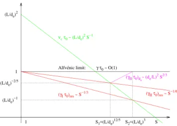
The three collisionality regimes are summarized in Fig.1. Here, the green line indicates the normalised collision frequency as a function of the Lundquist number. The red lines represent the growth rates in the resistive regime. When they are below the green line, the growth rate is smaller than the collision frequency and the resistive theory holds. One can see from the figure that forS <_ðL0=deÞ12=5both the

pri-mary and the secondary instability can be treated with

resistive MHD. On the other hand, whenS >_ðL0=deÞ3, none

of the growth rates is less than the collision frequency, and noncollisional effects must be taken into account. Finally, in the intermediate regime_ðL0=deÞ12=5< S <ðL0=deÞ3, the

pri-mary instability is resistive, but noncollisional effects are necessary to treat the secondary instability, whose growth rate is given by the mauve line.

The effect of non-collisional physics can be evaluated by considering the model with electron inertia22and adapt-ing the estimates of Sec. II (cf. Eqs. (C10)–(C13) in Appendix C). Then, by using againD0! 1=ka2_{, andR! L}

0,

Eqs.(8)–(11)are replaced by

cTs0! d3 eL0 a4 # $ kL0 ð Þ(1; (34) dT L0 ! d2 e a2 # $ kL0 ð Þ(1; (35) cKs0! de L0 # $ kL0 ð Þ; (36) dK L0 ! de L0 : (37)

The growth rate and the layer width as a function of the wavenumber are sketched in the log-log plot in Fig.2for the collisional (Eqs. (8)–(11) with D0 given by (12)) and non-collisional regime (Eqs.(34)–(37)).

In the intermediate regime, the situation with the two (collisional and non-collisional) estimates is summarized in Fig.3.

One can see that, apart from a range at the largest wave-numbers, the growth rate of the secondary instability is determined by non-collisional physics. In particular, the peak growth rate, occurring at the transition between (34) and(36), scales like

cMs0!

d2 e

a2: (38)

FIG. 1. Sketch in log-log scale of the maximum growth rate of the second-ary instability as a function of the Lundquist number in the collisional (red) and in the non-collisional (mauve) regime. Also shown are the growth rate of the primary instability (also red) and the collision frequency (green). Here,L0! L has been specified.

As one approaches the right boundary of the intermediate regime, the thickness of the primary layer decreases, we recall, as _!L0S(1=3. Thus, the maximum growth rate of the

secondary instability grows again as _!S2=3. This behavior is also shown in Fig. 1 (mauve line _ðcIIs0Þde). At the right

boundary of this regime,S_{! ðL}0=deÞ3anda! de. Then, the

current sheet produced by the primary instability approaches the electron skin depth, whilethe maximum growth rate of the secondary instability approaches Alfv!enic values.

The growth rate (38) is fast enough to account for the observed sawtooth crash time in a machine like JET.19These observations call for a non-collisional theory since the observed rates are faster than the collision frequency. In this respect, referring again to Fig.1, we notice that our approach brings the boundary, beyond which the collisionless effects matter, down toS_{! ðR=d}eÞ12=5. This value of the Lundquist

number is much more easily achieved in large tokamaks than S_{! ðR=d}eÞ3at which the primary instability enters the

colli-sionless regime (upper boundary of the intermediate regime). One can also remark that the reconnection rate has a mini-mum that scales like_!ðde=L0Þ2=5, in Alfv!en units, in all

col-lisionality regimes.

IV. DISCUSSION AND CONCLUSIONS

The results of Yuet al.26have also been interpreted27in terms of the plasmoid instability.3However, it appears that the literature on the plasmoid instability does not take into account the rescaling of the current sheet magnetic field with respect to its macroscopic, reference value (Eq. (1)) and, under these hypotheses, the assumption that the current layer aspect ratio scalesa-la Sweet-Parker, which is at the basis of" the plasmoid instability scaling,3,6,10,34 becomes question-able.6We recall that the rescaling(1)is necessary to estimate correctly the size of the current sheet magnetic field at the end of the linear phase of a primary instability such as the m_{¼ n ¼ 1 mode in the sawtooth phenomenon.}

By ignoring such rescaling, the secondary instability is faster, such that the maximum growth rate given in Eq.(14) would be replaced by6 cMs0! S( 1 2 0 L0 a # $3 2 : (39)

By assuming that the width of the current sheet resulting from the primary instability scales like _!S(1=3_R , as in this work, together with estimate (39), one would conclude that the maximum growth rate scales like the ideal tearing growth ratecIIs0 ! Oð1Þ, independent of resistivity.

These assumptions are at the root of the work of Pucci and Velli as a criterion for anideal tearing reconnection rate in a purely resistive model.6,8,9

If on the other hand one assumed a narrower current layer scaling a-la Sweet-Parker, a" _{! L}0S(1=20 , and at the

same time one ignored the rescaling (Eq.(1)), thereby using again estimate (39), one would end up with a faster-than Alfv_{!enic estimate of the maximum growth rate !S}1=4₀ , which gives, forL0¼ L, the plasmoid instability scaling.28

Therefore, in the scenario where the current sheet is pro-duced by a primary instability, as in the sawtooth case, we consider the results based on the plasmoid instability unlikely, since we have shown that the current sheet becomes sufficiently

FIG. 2. Growth rate, layer width, andD0 _{as a function of the wavenumber}

for the collisional (a) and the non-collisional (b) theory.L0! L has been

specified.

FIG. 3. The scalings of the resistive (label “res”) and of the purely inertia-driven (label “de”) regimes atL¼ L0and forðL=deÞ12=5< S <ðL=deÞ3 are,

respectively, given by(10)and(36)for the primary growth rates (cIs0) and by

(8) and(34) for the growth rates of the secondary tearing modes (cTs0).

Similarly,(11),(37)and(9),(35)respectively give the inner layer widthsdI=L

unstable to secondary sub-Alfv!enic modes at an earlier stage in its development and it would therefore likely break up before becoming sharper, in current concentration, or thinner, in width, than the estimates of Eqs. (1) and (11), respectively.

In summary, in this work, we have shown that a current sheet generated by a primary instability, such as the internal kink mode, becomes sufficiently unstable at an early stage in its nonlinear development.

When applied to the context of the sawtooth phenome-non, the analysis of the secondary instability reveals that the sawtooth crash due to reconnection proceeds at a faster rate than previous estimates based on the primary m¼ n ¼ 1 internal kink mode.22In the case of a purely resistive model, the reconnection rate depends weakly on the Lundquist num-ber,_!S(1=6, and it appears in agreement with the results of numerical simulations at a large Lundquist number.26 Also, the value of the Lundquist number at which collisionless effects become important is found to be substantially lower than the estimate based on the primary instability only. This broadens the range of tokamaks to which collisionless effects should be taken into account in the analysis of the sawtooth phenomenon. Finally, near-Alfv!enic reconnection rates can be achieved by secondary instabilities when collisionless effects become important also for the primary instability.

The scope of this work is to outline a possible scenario for fast reconnection, and in this respect, scaling estimates are useful, and sufficient for a first investigation.

Detailed stability analysis of current sheets, taking into account the actual geometry, such as them_{¼ 1 ribbon, is a} possibility to obtain more precise predictions about the maxi-mum growth rate, the associated wavenumber, and the insta-bility threshold. This might lead to an explanation of the Lundquist number threshold observed in numerical simula-tions26and of the number of observed secondary islands.

The effect of flows also merits an investigation. In this respect, one notes that flows are small near the primary instabil-ityX-point, which is a stagnation point, but may be significant far from it, potentially leading to stabilizing effects on the tear-ing mode9,29–31and/or to additional instabilities such as Kelvin-Helmholtz’s.32–34 In particular, according to Bulanov et al.30 and Syrovatskii,31flow stabilization would occur if its deriva-tive along the reconnection line would roughly exceed the insta-bility growth rate. Our estimates indicate that the former scales likeS(1=3₀ at the end of the linear phase of the primary instabil-ity, whereas the latter scales, as we have seen, at least asS(1=6₀ . Thus, the criterion is not met and the flow can be neglected.

Finally, the stability analysis carried out in this work is based on a magnetic configuration with the current aligned to a main magnetic field. Relaxing this hypothesis and allow-ing for pressure gradients would open further possibilities.

ACKNOWLEDGMENTS

The authors wish to thank Q. Yu for discussions about his work, A. Tenerani for interesting discussions and for details about Ref. 9, and L. Comisso for having brought attention to Ref.28. Discussions with F. Pucci and M. Velli on the ideal tearing are also gratefully acknowledged.

APPENDIX A: NOTIONS OF FAST RECONNECTION

For the sake of clarity, let us briefly review the use of the adjective “fast” in the context of the reconnection litera-ture, since its meaning has been changing over the years and in different contexts.

Until about the 1990s, especially in tokamak-related litera-ture, “fast” refers to a reconnection rate that is faster than what is expected by the resistive tearing mode13 and Sweet-Parker35,36scalings, which are too slow to account for experi-mental evidence.19From the theoretical viewpoint, “fast” refers to effects beyond resistive MHD, such as electron inertia,20–22 that allow a finite reconnection rate even when the resistivity is negligibly small. This is the meaning adopted in this work. We also note that the word “collisionless” has been frequently used for this latter purpose, too, but while in origin it meant a recon-nection triggered by (electron) inertia effects replacing resistiv-ity (see, e.g., Refs.21,22,37, and58), it has later been used to generically underline the role of collisionless effects, in particu-lar, the Hall-term, inenhancing resistivity-driven reconnection rates (see, e.g., Refs. 39–41). This change of terminology relates to that for the notion of fast reconnection.

In more recent literature, the word “fast” seems to have taken the more restrictive meaning of reconnection at ideal time scales (Alfv!enic or even super-Alfv!enic), essentially after the whistler-mediated (or Hall-mediated) reconnection model,38,39

displaying a reconnection rate weakly dependent on the non-ideal parameters, has been recognized as the par-adigm for magnetospheric reconnection.40–42

We recall however that the Hall-term is negligible in the strong guide field, slab geometry approximation pertinent to tokamaks and considered here, where it is related at most to ion-sound Larmor radius effects (see, e.g., Refs. 10 and 43–45), well known to increase the “cold” resistive recon-nection rate21 but without allowing the transition to the whistler-mediated regime.

Starting from the 2000s, different models for this more recent meaning of “fast” reconnection have been then consid-ered as relevant to secondary reconnection events: the plas-moid-induced, fractal reconnection model,1

which the more recent plasmoid instability3 is reminiscent of, and then the “ideal” tearing model.6As discussed in the recent review 11, however, all of them essentially consist of tearing-type insta-bilities that generate “plasmoids,” i.e., magnetic islands, with different growth rate scalings that depend on the scalings of the current sheet aspect ratio. In this regard, it is in Ref.6that a distinction was first made between reconnecting modes clas-sified as “slow” (i.e., ideally stable), “fast” (i.e., (quasi-)ide-ally unstable), and “violently unstable” (i.e., with diverging growth rates while approaching the ideal limit).

APPENDIX B: BRIEF REVIEW OF NUMERICAL RESULTS AND EXPERIMENTAL OBSERVATIONS OF SECONDARY RECONNECTING INSTABILITIES

As the notion of secondary reconnection requires the primary reconnection event to be treated as relatively “stationary” with respect to the secondary growth rate (s(1

rec;I$ cII), it is natural that such an occurrence has been

first evidenced as generation of “plasmoids” on almost sta-tionary current-sheets that were reconnecting "a la Sweet-Parker48,49 or developing between two coalescing magnetic islands50(see also Ref.14). For long time, secondary recon-nection has been thus refereed to primary Sweet-Parker-like reconnection rates. It is in this sense, for example, that radio pulsations measured in solar flares have been related to the dynamics of magnetic islands secondarily generated on a quasi-stationary reconnecting current sheet.51

On the other hand, it was known from the theoretical works by Syrovatskii52 (see also Ref. 31 and references therein) that current sheets could form from the collapse of an X-point into the so-called two-Y-point configuration. Besides the coalescence instability problem,46,47 where the collapse of theX-point in-between two coalescing flux ropes is driven by the mutual attraction of the two current patches, the double-Y-point configuration could naturally evolve from X-points generated by primary tearing modes. Evidence of this was provided, for example, in the numerical studies of the nonlinear tearing mode22,23,58(see, in particular, Fig. 13 of Ref. 23), whose dynamics had been already shown by analysis to imply the formation of a current sheet,24 or in studies dedicated to the investigation of the X-point col-lapse.53 The computational resources available a few years later allowed us to evidence the occurrence of secondary instabilities: fluid-type instabilities were shown to affect the current sheet evolution in a primary collisionless internal kink mode32or in large wave-length EMHD reconnection,54 in agreement33 with the importance of the electron Kelvin-Helmholtz mode for the instability of thin current layers in collisionless regimes.55Then, in resistive regimes, also sec-ondary reconnecting instabilities were shown to occur: it is essentially after Refs. 2, 56, and 57, which showed an increase of the reconnection rate due to the formation of plasmoids in the current sheet generated by the collapse of magnetic island X-points, that the secondary reconnection rate started being compared to primary tearing-type modes, too. It is also worth noticing that, looking retrospectively, Aydemir’s early numerical investigation of the internal kink in cylindrical geometry58 contains elements of secondary instabilities in a collision-less regime, although at the time different interpretations were sought for the observed recon-nection rate increase.

While this seems to summarize the main stream of plasma literature on secondary reconnection until about the first half decade of the 2000s, we note that more specifically astrophysic-oriented works had already evidenced1,59 how fast, secondary tearing modes could develop on the current sheet generated during the nonlinear evolution of a primary tearing (in turn induced, in the case studied in Ref.59, by a shock-wave trespassing a current sheet). Some specific words are due, in particular, to the pioneering works by Shibata and Tanuma, who, between the end of 1990s and begin of 2000s, devised the plasmoid-induced reconnec-tion1,60

and the fractal reconnection1

models to account for nonlinear fast reconnection processes: the former highlights the role of plasmoids, generated by primary reconnection events and ejected along the current sheet, in enhancing the inflow and thus the reconnection rate atX-points because of

mass conservation between the inflow and outflow. The latter considers how this may contribute to a cascade, fractal-like pro-cess, in which a sequence of increasingly faster tearing modes develop each on the shoulder of the previous one, after a suffi-ciently large aspect ratio current sheet has formed from the X-point collapse of each tearing. A re-scaling argument analogous to the one discussed here and the assumption of a Sweet-Parker scaling for each current sheet aspect ratio are two ingredients of this model, in which the growth rate of a secondary tearing was probably first compared to a previous one.

The interpretation of the current sheet generated by the X-point collapse as a Sweet-Parker state, also assumed in Refs.2and53, led a few years later to the formalization of theplasmoid instability,3

which thereafter became indicative of a specific positive scaling ofc with S in the strong guide field, slab geometry approximation (for a brief review of the previous usage of the term “plasmoid” in reconnection, espe-cially in astrophysics, see, e.g., Ref. 62). As Tajima and Shibata earlier pointed out,28 however, cs0! S1=40 and

kML! S3=80 are the scalings of the most unstable tearing

mode in a Sweet-Parker current sheet when L0¼ L, fact

which highlights the tearing nature of theplasmoid instabil-ity. After Ref.3, many numerical results, starting from Refs. 16 and 61, have been interpreted in terms of the plasmoid instability scaling, including27 the recent results by Yu and co-workers26on the nonlinear evolution of an internal kink mode during the sawtooth cycle in a purely resistive regime.

Alternative interpretations have been nevertheless pro-vided for the almost ideal reconnection rates(1

recs0 ! Sa0with

a ’ 0, often numerically measured in correspondence of the generation of secondary islands (see, e.g., Refs. 8–11, 27, and63–70), which are based on 3D effects, on reconnection mechanisms of kinetic nature and/or on two-fluid effects, or on the linear or quasi-linear analysis of secondary reconnect-ing modes. Some of the latter have been sought followreconnect-ing the recent criticism to the Sweet-Parker scaling assump-tion—see in this regard the “ideal”-tearing based mod-els,6–11 which first have raised it in evidencing a threshold aspect ratio of the current sheet to ideal reconnection rates that is smaller thanL=a_{! S}1=2_{, and Refs.69and70.}

In particular, numerical evidence of two “ideal” tearing modes, developing in sequence, one secondary to the other, has been first provided in Ref.8. In Ref. 9, this mechanism has been shown to iterate in a cascade process akin to the frac-tal reconnection model (see also Ref.11for a comparison of the two), in which the stabilizing role of flows becomes pro-gressively more important. The assumption Bcs! B0, which

implies Jcs, J0 whenL0=a, 1, seems to be verified9,11in

these models, of which it is a key ingredient. As we have already pointed out, this is not the case for the current sheet generated by primary “non-ideal” resistive tearing modes, for whichJcsis disrupted by secondary instabilities before it over-takes too much the macroscopic current sheet J0. Therefore, the estimation provided in Ref.10to account for the possible onset of a secondary “ideal” regime by starting from a pri-mary “non-ideal” tearing mode or for the secondary reconnec-tion rate increase, sometimes evidenced in simulareconnec-tions as the explosive reconnection regime,64,66

should be corrected in the light of Eqs.(8)–(11),(C10)–(C13).

Regardless of the assumptions implying different scaling estimations, the reconnecting instabilities leading to second-ary magnetic island formation can be essentially treated as tearing-type modes (see, e.g., Ref. 11), as long as a WKB-type approach makes it possible to apply a linear instability analysis on a relatively slowly evolving current sheet.

Secondary magnetic islands generated next to X-points of primary reconnecting modes have been observed also in numerical simulations of turbulent reconnection71and have been evidenced byin situ satellite measurements in the mag-netosphere.72,73 The formation of secondary islands, due to the nonlinear reconnection of magnetic lines on different rational surfaces, has also been pointed out in early numeri-cal studies of the double-tearing mode in the collision-less regime,74and, more recently, the reconnection rate has been observed to abruptly increase during the nonlinear stage of a primary double-tearing mode up to almost ideal scalings75–77 In Ref.77, in particular, a geometrical threshold to the onset of secondary linear modes, growing almost independent ofS, has been identified in terms of the 2D structure that the pri-mary magnetic islands achieve during the nonlinear evolu-tion of the initial double-tearing.

A cascade of reconnecting instabilities from an initial reconnecting mode at macroscopic scales down to reconnection below the ion-skin depth scale has been evidenced by Moser and Bellan in laboratory experiments of a magnetized current carrying plasma jet.81More recently, plasmoid generation due to a secondary resistive tearing on a current sheet generated by driven, quasi-steady reconnection, has been measured in experi-ments with the MRX device.78Thanks to the recent improve-ments of the diagnostic systems, and, in particular, of the soft X-ray and electron cyclotron emission imaging, also the growth of secondary reconnecting instabilities during the sawtooth phe-nomenon in tokamaks (itself known since the first observations reported in Ref. 18) has been experimentally measured. Examples are provided by Ref.79for the HT-7 device and by Ref.80for the ASDEX-Upgrade tokamak.

APPENDIX C: SOME ELEMENTS OF THE STABILITY ANALYSIS

In this appendix, we review the stability analysis of Eqs. (4)and(5)with the asymptotic matching technique. We give only the key elements as the procedure is already known. In the region around the boundary layer at x_{¼ 0, such that} x_{$ L}0, called theinner region, we can approximate the

par-allel derivative operator as in Eq.(6)

rjjeq -B0csð Þ0 B0 # $ x@y¼ x L0 # $ @y; (C1)

where the shear lengthLs) B0=B0csð0Þ can be identified with

the generic macroscopic scale lengthL0for our purposes. Consider then perturbations of the form ^_{w ! e}ct_cosðkyÞ

and ^_{/ ! e}ctsin_{ðkyÞ. Assume also a strong radial variation} across the boundary layer, such that in the inner region one can take @x, k, and keep only the leading terms. Then,

Eqs.(4)and(5)become

1 c2 A c^/00¼ k _Lx 0 # $ ^ w00; (C2) c ^w ( d2 ew^ 00 ! " þ k _Lx 0 # $ ^ / ¼ ^g ^w00: (C3)

Here, the electron inertia term proportional to the square of the electron skin depthdehas been introduced as a first step to include noncollisional effects.

By first defining a length de such that d2e) de2þ ^g=c,

and then by introducing the parameter Q_{) cL}0=ðkCAdeÞ,

and the length dL) Q1=2de, one can recast Eqs. (C2) and

(C3)in the form ^ /00R¼ 1 QxRw^R 00_{; (C4)} ^ wRþ xR/^R ¼ 1 Qw^R 00_{; (C5)} where xR¼ x=dL;/RðxRÞ ¼ kdL/ðdLxRÞ=ðL0cÞ, and wRðxRÞ

¼ wðdLxRÞ. The parameter Q can be considered as an

eigen-value, whiledL is an effective layer width, itself implicitly dependent on the eigenvalue. In general, one can assume dL$ L0. Thus, there exists an overlapping region dL$ x

$ L0 where both Eqs. (C2) and (C3) and the ideal MHD

equations (outer equations) are valid. Matching the expres-sions of the solutions of these two sets of equations in the overlapping region fixes the eigenvalue and the layer width.

The solution of Eqs. (C4) and (C5) was obtained in a closed form, by means of an integral representation, by Coppi et al.,82 _{while a detailed calculation is given in the}

appendix of Ref. 83. An alternative method,84 which turns out useful to treat more general models,21,23,85,86is based on Fourier transforms in the variablexR.

In the overlapping region, the leading asymptotic expan-sions of the two functions take the form

^ wR ! w1 1þ D0 2x # $ (C6) ^ /R ! /1 1( 2kH p 1 x # $ ; (C7)

where the quantitykHis a normalised version of the potential energy variationdW arising in the energy principle.

The above relations are those pertinent to this work, which is unstable tearing modes (D0> 0), but stable ideal modes (kH< 0).

By inspecting Ohm’s law(C5)in the overlapping region xR, 1, one can see that the following relation holds:

1_{¼ (D}0kH

p : (C8)

The eigenvalue condition of Ref.82 rewritten in terms of23Q andD0can be conveniently recast in the form

D0dL¼ (p

8Q

C Q ( 1(ð Þ=4)

C Q þ 5(ð Þ=4) : (C9)

From this equation, the scaling of the different D0 regimes can be immediately recovered. In particular, for D0dL! 0, where dL! dT, one has to take Q! 0. In the

resistive regime, one takesde¼ 0 so that d2e¼ ^g=c. One then

recovers the scaling (8)for the growth rate and the scaling (9)for the layer width. In the opposite limit, whenD0dL! 1

anddL! dK, one has to takeQ! 1, to approach the pole of

the C function. The result is then the scaling (10) for the growth rate and the scaling(11)for the layer width. Similarly, in the collisionless regime, one takes^_{g ¼ 0; d}e¼ de, and one

recovers the collisionless scaling used in the last part of this work.

Finally, we draw the attention to the fact that the scaling ofQ can also be estimated directly from Eqs.(C4)and(C5) without carrying out a detailed matching calculation, by tak-ing the constant-w scaling w00R ! D0dLwR for smallD0and the

natural scalingw00

R ! wRin the largeD0limit. Then, the

con-dition that all the terms of Eqs. (C4)and(C5) are balanced requires assumingQ_{! D}0dLandQ! 1 in the two respective

regimes. In this way, one makes direct contact with the colli-sional estimates given in Sec.II.

The corresponding scaling in the collisionless regime is

cTs0! ðkdeÞðD0deÞ2; (C10) dT L0! de L0 # $2 D0_L 0 ð Þ; (C11) cKs0 ! kde; (C12) dK L0 ! de L0 : (C13)

This latter scaling has been used to derive the estimates in Eqs.(34)–(37).

1_{K. Shibata and S. Tanuma,Earth Planets Space}

53, 473 (2001).

2_{N. F. Loureiro, S. C. Cowley, W. D. Dorland, M. G. Haines, and A. A.} Scheckochihin,Phys. Rev. Lett.95, 235003 (2005).

3_{N. F. Loureiro, A. A. Scheckochihin, and S. C. Cowley,Phys. Plasmas} 14, 100703 (2007).

4_{W. Daughton, V. Roytershteyn, B. J. Albright, H. Karimabadi, L. Yin, and} K. J. Bowers,Phys. Rev. Lett.103, 065004 (2009).

5_{D. Uzdensky, N. F. Loureiro, and A. A. Scheckochihin,Phys. Rev. Lett.} 105, 235002 (2010).

6_{F. Pucci and M. Velli,Astrophys. J. Lett.}

780, L19 (2014).

7_{A. Tenerani, A. F. Rappazzo, M. Velli, and F. Pucci,Astrophys. J.} 801, 145 (2015).

8_{S. Landi, L. Del Zanna, E. Papini, F. Pucci, and M. Velli,Astrophys. J.} 806, 131 (2015).

9_{A. Tenerani, M. Velli, A. F. Rappazzo, and F. Pucci,Astrophys. J. Lett.} 813, L32 (2015).

10_{D. Del Sarto, F. Pucci, A. Tenerani, and M. Velli,J. Geophys. Res.} 121, 1857, doi:10.1002/2015JA021975 (2016).

11_{A. Tenerani, M. Velli, F. Pucci, S. Landi, and A. F. Rappazzo,J. Plasma}

Phys.82, 535820501 (2016).

12_{P. A. Cassak and J. F. Drake,Astrophys. J.}

707, L158 (2009). 13_{H. Furth, J. Killeen, and M. N. Rosenbluth,Phys. Fluids}

6, 459 (1963). 14

E. R. Priest,Rep. Prog. Phys.48, 955 (1985). 15

M. Velli and A. W. Hood,Solar Phys.119, 107 (1989).

16_{A. Battacharjee, Y.-M. Huang, H. Yang, and B. N. Rogers,Phys. Plasmas} 16, 112102 (2009).

17_{E. G. Harris,Il Nuovo Cimento}

23, 115 (1962).

18_{S. Von Goeler, W. Stodiek, and N. Sauthoff,Phys. Rev. Lett.} 33, 1201 (1974).

19

A. W. Edwards, D. J. Campbell, W. W. Engelhardt, H.-U. Fahrbach, R. D. Gill, R. S. Granetz, S. Tsuji, B. J. D. Tubbing, A. Weller, J. Wesson, and D. Zasche,Phys. Rev. Lett.57, 210 (1986).

20

J. Wesson,Nucl. Fusion30, 2545 (1990). 21_{F. Porcelli,Phys. Rev. Lett.}

66, 425 (1991). 22_{M. Ottaviani and F. Porcelli,Phys. Rev. Lett.}

71, 3802 (1993). 23

M. Ottaviani and F. Porcelli,Phys. Plasmas2, 4104 (1995). 24

F. L. Waelbroeck,Phys. Fluids B1, 2372 (1989). 25_{F. L. Waelbroeck,Phys. Rev. Lett.}

70, 3259 (1993). 26

Q. Yu, S. G€unter, and K. Lackner,Nucl. Fusion54, 072005 (2014). 27

S. G€unter, Q. Yu, K. Lackner, A. Bhattacharjee, and Y. M. Huang,Plasma Phys. Controlled Fusion57, 014017 (2015).

28_{T. Tajima and K. Shibata,}

Plasma Astrophysics (Addison-Wesley, 1997), p. 229.

29_{D. Biskamp,}

Magnetic Reconnection in Plasmas (Cambridge University Press, 2000).

30

S. V. Bulanov, J. Sakai, and S. I. Syrovatskii, Sov. J. Plasma Phys.5, 157 (1979).

31_{S. I. Syrovatskii,Rev. Astron. Astrophys.}

19, 163 (1981). 32

D. Del Sarto, F. Califano, and F. Pegoraro,Phys. Rev. Lett.91, 235001 (2003).

33_{D. Del Sarto, F. Califano, and F. Pegoraro,Mod. Phys. Lett. B} 20, 931 (2006).

34_{N. F. Loureiro, A. A. Schekochihin, and D. A. Uzdensky,Phys. Rev. E} 87, 013102 (2013).

35

P. A. Sweet, inElectromagnetic Phenomena in Cosmical Physics, edited by B. Lehnert (IAU Symposium, 1958) Vol. 6, p. 123.

36_{E. N. Parker, J. Geophys. Res.}

62, 509–520, doi:10.1029/ JZ062i004p00509 (1957).

37_{J. F. Drake and R. G. Kleva,Phys. Rev. Lett.}

66, 1458 (1991). 38_{M. E. Mandt, R. E. Denton, and J. F. Drake,Geophys. Res. Lett.}

21, L73, doi:10.1029/93GL03382 (1994).

39_{D. Biskamp, E. Schwarz, and J. F. Drake, Phys. Rev. Lett.}

75, 3850 (1995).

40

M. A. Shay, J. F. Drake, B. N. Rogers, and R. E. Denton,J. Geophys. Res.-Space106, 3759 (2001).

41_{M. Hesse, J. Birn, and M. Kuznetsova, J. Geophys. Res.}

106, 3721, doi:10.1029/1999JA001002 (2001).

42_{J. Birn, J. F. Drake, A. Shay, B. N. Rogers, R. E. Denton, M. Hesse, M.} Kuznetsova, Z. W. Ma, A. Battacharjee, A. Otto, and L. Pritchett,

J. Geophys. Res.106, 3715, doi:10.1029/1999JA900449 (2001). 43_{X. Wang and A. Battacharjee,Phys. Rev. Lett.}

70, 1627 (1993). 44

R. G. Kleva, J. F. Drake, and F. L. Waelbroeck,Phys. Plasmas 2, 23 (1995).

45_{R. Fitzpatrick and F. Porcelli,Phys. Plasmas}

11, 4713 (2004); 14,049902

(2007).

46_{J. M. Finn and P. K. Kaw,Phys. Fluids}

20, 72 (1977). 47_{P. L. Pritchett and C. C. Wu,Phys. Fluids}

22, 2140 (1979).

48_{B. U. O. Sonnerup and J.-I. Sakai, EOS Trans. Am. Geophys. Union} 62, 353 (1981).

49_{D. Biskamp, Z. Naturforsch.}

37a, 840 (1982). 50_{D. Biskamp,Phys. Lett.}

87 A, 357 (1982). 51

B. Kliem, M. Karlick!y, and A. O. Benz, Astron. Astrophys. 360, 715 (2000), available at http://aa.springer.de/papers/0360002/2300715/small. htm.

52

S. I. Syrovatskii, Sov. Phys. JETP33, 933 (1971), available athttp://jetp. ac.ru/cgi-bin/dn/e_033_05_0933.pdf.

53_{B. D. Jemella, M. A. Shay, J. F. Drake, and B. N. Rogers,Phys. Rev. Lett.} 91, 125002 (2003).

54_{D. Del Sarto, F. Califano, and F. Pegoraro, Phys. Plasmas}

12, 012317 (2005).

55

J. F. Drake, R. G. Kleva, and M. E. Mandt,Phys. Rev. Lett.73, 1251 (1994).

56

J. F. Drake, M. Swisdak, K. M. Schoeffler, B. N. Rogers, and S. Kobayashi,Geophys. Res. Lett.33, L13105, doi:10.1029/2006GL025957 (2006).

57

W. Daughton, J. Scudder, and H. Karimabadi,Phys. Plasmas13, 072101 (2006).

58_{A. Y. Aydemir,Phys. Fluids B}

4, 3469 (1992). 59

S. Tanuma, T. Yokoyama, T. Kudoh, and K. Shibata,Astrophys. J.551, 312 (2001).

60_{K. Shibata,Adv. Space Res.}

17, 9 (1996). 61

R. Samtaney, N. F. Loureiro, D. A. Uzdensky, A. A. Schekochihin, and S. C. Cowley,Phys. Rev. Lett.103, 105004 (2009).

62

J. Lin, S. R. Cranmer, and C. J. Farrugia,J. Geophys. Res.113, A11107, doi:10.1029/2008JA013409 (2008).

63_{G. Lapenta,Phys. Rev. Lett.}

100, 235001 (2008). 64

A. Biancalani and B. D. Scott,Europhys. Lett.97, 15005 (2012). 65

L. Comisso, D. Grasso, F. L. Waelbroeck, and D. Borgogno, Phys. Plasmas20, 092118 (2013).

66_{A. Ali, J. Li, and Y. Kishimoto,Phys. Plasmas}

21, 052312 (2014). 67

P. A. Cassak, R. N. Taylor, R. L. Fermo, M. T. Beidler, M. A. Shay, M. Swidsak, J. F. Drake, and H. Karimabadi, Phys. Plasmas 22, 020705 (2015).

68_{M. Hirota, Y. Hattori, and P. J. Morrison, Phys. Plasmas}

22, 052114 (2015).

69

D. A. Uzdensky and N. F. Loureiro,Phys. Rev. Lett.116, 105003 (2016). 70_{L. Comisso, M. Lingham, Y. M. Huang, and A. Battacharjee, Phys.}

Plasmas23, 100702 (2016). 71

M. Wan, A. F. Rappazzo, W. H. Matthaeus, S. Servidio, and S. Oughton,

Astrophys. J.797, 63 (2014).

72_{J. P. Eastwood, T.-D. Phan, F. S. Mozer, M. A. Shay, M. Fujimoto, A.} Retin"o, M. Hesse, A. Balogh, E. A. Lucek, and I. Dandouras,J. Geophys. Res.112, A6235, doi:10.1029/2006JA012158 (2007).

73

R. Wang, Q. Ly, A. Du, and S. Wang, Phys. Res. Lett. 104, 175003 (2010).

74_{A. T. Lin,Phys. Fluids}

21, 1026 (1978).

75

Y. Ishi, M. Azumi, and Y. Kishimoto, Phys. Rev. Lett. 89, 205002 (2002).

76_{Z. X. Wang, X. G. Wang, J. Q. Dong, Y. A. Lei, Y. X. Long, Z. Z. Mou,} and W. X. Qu,Phys. Rev. Lett.99, 185004 (2007).

77

M. Janvier, Y. Kishimoto, and J. Q. Li,Phys. Rev. Lett. 107, 195001 (2011).

78_{J. Jara-Almonte, H. Ji, M. Yamada, J. Yoo, and W. Fox,Phys. Rev. Lett.} 117, 095001 (2016).

79

X. Xu, J. Wang, Y. Wen, Y. Yu. A. Liu, T. Lan, C. Yu, B. Wan, X. Gao, Y. Sun, N. C. Luhmann, Jr., C. W. Domier, Z. G. Xia, and Z. Shen,

Plasma Phys. Controlled Fusion52, 015008 (2010). 80

V. Igochine, J. Boom, I. Classen, O. Dumbrajs, S. G€unter, K. Lackner, G. Pereverzev, H. Zohm, and ASDEX Upgrade Team,Phys. Plasmas 17, 122506 (2010).

81_{A. L. Moser and P. M. Bellan,Nature}

482, 379 (2012). 82

B. Coppi, R. Galv~ao, R. Pellat, M. Rosenbluth, and P. Rutherford, Fiz. Plazmy2, 961 (1976).

83_{G. Ara, B. Basu, and B. Coppi,Ann. Phys.}

112, 443 (1978). 84_{F. Pegoraro and T. J. Schep, Plasma Phys. Controlled Fusion}

4, 667 (1986).

85

F. Pegoraro, F. Porcelli, and T. J. Schep,Phys. Fluids B1, 364 (1989). 86_{S. V. Bulanov, F. Pegoraro, and A. S. Sakharov,Phys. Fluids B}

28, 647 (1992).