HAL Id: hal-02947772
https://hal.sorbonne-universite.fr/hal-02947772
Submitted on 24 Sep 2020
HAL is a multi-disciplinary open access
archive for the deposit and dissemination of
sci-entific research documents, whether they are
pub-lished or not. The documents may come from
teaching and research institutions in France or
abroad, or from public or private research centers.
L’archive ouverte pluridisciplinaire HAL, est
destinée au dépôt et à la diffusion de documents
scientifiques de niveau recherche, publiés ou non,
émanant des établissements d’enseignement et de
recherche français ou étrangers, des laboratoires
publics ou privés.
two-dimensional shear flow
Vassilios Dallas, Kannabiran Seshasayanan, Stephan Fauve
To cite this version:
Vassilios Dallas, Kannabiran Seshasayanan, Stephan Fauve. Transitions between turbulent states
in a two-dimensional shear flow. Physical Review Fluids, American Physical Society, 2020, 5 (8),
�10.1103/PhysRevFluids.5.084610�. �hal-02947772�
Vassilios Dallas,1, ∗ Kannabiran Seshasayanan,2, † and Stephan Fauve3, ‡
1
Mathematical Institute, University of Oxford, Woodstock Road, Oxford OX2 6GG, UK
2Service de Physique de l’Etat Condens´e (SPEC), CEA Saclay Bˆatiment 772,
Orme des Merisiers, F-91191 Gif sur Yvette Cedex, France
3
Laboratoire de Physique de l’ ´Ecole normale sup´erieure, ENS, Universit´e PSL, CNRS, Sorbonne Universit´e, Universit´e Paris-Diderot, Sorbonne Paris Cit´e, Paris
We study the bifurcations of the large scale jets in the turbulent regime of a forced shear flow using direct numerical simulations of the Navier-Stokes equations. The bifurcations are seen in the probability density function (PDF) of the largest scale mode with the control parameter being the Reynolds number based on the friction coefficient denoted as Rh. As one increases Rh in the turbulent regime, the PDF of the large scale mode first bifurcates from a Gaussian to a bimodal behaviour, signifying the emergence of reversals of the large scale flow where the flow fluctuates between two distinct turbulent states. Further increase in Rh leads to a bifurcation from bimodal to unimodal PDF which denotes the disappearance of the reversals of the largest scale mode. We attribute the latter transition to the long-time memory that the large scale flow exhibits related to low frequency 1/fαtype of noise with 0 < α < 2. We also demonstrate that a minimal model with 15 modes, obtained from the truncated Euler equation, is able to capture the bifurcations of the large scale jets exhibited by the Navier-Stokes equations.
Keywords: bifurcations, truncated Euler equation, 1/f noise, Kolmogorov flow
I. INTRODUCTION
Low-frequency variability in climate exhibits recurrent patterns that are directly linked to dynamical processes of the governing dissipative system [1, 2]. The study of the persistence of these large scale patterns and the transitions between them plays a crucial role in understanding climate change [3]. Climate variability is often associated with dynamic transitions between different regimes, each represented by local attractors. Examples of climate phenomena where such transitions have been investigated experimentally as well as numerically are the transitions between different mean flow patterns of the Kuroshio Current in the North Pacific [4, 5], the transitions between blocked and zonal flows in the midlatitude atmosphere [6], and the transition to oscillatory behaviour in models of Quasi-biennial oscillations [7, 8].
Understanding naturally occurring bifurcations in climate systems through observational studies is challenging due to the lack of control on the different physical processes involved. Numerical and experimental studies that model such systems can overcome such difficulties to study these bifurcations, where the parameters can be systematically controlled. They can provide important insights for our understanding of the behaviour observed in the natural counterparts. Models varying from idealised systems to the global climate models succeed in reproducing some of the observed phenomena. Such complex transition and bifurcations have also been observed in many idealised fluid mechanical systems. Bifurcations on turbulent flows have been observed in a range of experimental and numerical studies for flow past bluff bodies [9, 10], Rayleigh-B´enard convection with and without rotation [11–14], von Karman flow [15–17], reversals in a dynamo experiment [18] and experiments of dimensional turbulence [19]. The two-dimensional turbulence experiments showed the formation of a large scale condensate which displays a series of bifurcations. These were also seen in numerical simulations that mimic the experimental set-up [20].
Large scale zonal flows are found in planetary atmospheres and the ocean. Their existence motivates the study of jet formation in a turbulent flow driven at smaller scales. Anisotropy helps in the formation of these jet structures, which are usually introduced either by a β-plane that models the variation of the rotation with latitude [21], or by a domain of non-unity aspect ratio [22], or due to confinement and boundary conditions, see [23] and references therein. These large scale jets are known to be quite stable, evolving over longer time scales than the underlying turbulence. Such seemingly stable states undergo transitions at times [24], and modelling such phenomena remains an open question.
While much of the progress in fluid dynamics has been on hydrodynamic instabilities, only limited progress exists on transitions/instabilities that occur when a control parameter is varied within the turbulent regime, which is the focus
of this paper. The difficulty in studying such transitions arises from the underlying turbulent fluctuations which make any analytical progress cumbersome. These types of transitions resemble more closely phase transitions in statistical mechanics because the instability occurs on a fluctuating background [25]. A recent successful attempt [26] to model such transitions of the large scale circulation observed in experiments [19] involved a statistical mechanical theory at thermal equilibrium based on the truncated Euler equation (TEE) [27, 28].
In this paper we study the bifurcations of large scale jets in a two-dimensional shear flow confined in the latitudinal direction. Using direct numerical simulations of the Navier-Stokes equations we quantify the behaviour of the large scale mode and the bifurcations that occur in the turbulent regime. Finally, we systematically develop a minimal model using the truncated Euler equation to capture the large scale behaviour of the Navier-Stokes equations.
II. PROBLEM SET-UP
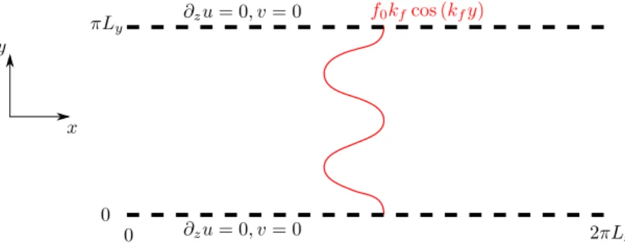
We consider the two-dimensional Navier-Stokes equations for an incompressible velocity fieldu = ∇ × ψˆz forced by a Kolmogorov type forcing in an anisotropic domain (x, y) ∈ [0, 2πLx] × [0, πLy] as illustrated in Fig. 1. The
governing equation written in terms of the streamfunction ψ(x, y, t) is given by,
∂tψ +∇−2{∇2ψ, ψ} = ν∇2ψ − µψ + f0sin(kfy) (1)
where {f, g} = fxgy− gxfy is the standard Poisson bracket (subscripts here denote differentation), ν is the kinematic
viscosity, µ is the friction coefficient, f0 is the amplitude of the Kolmogorov forcing and kf is the number of half
wavelengths in the forcing. Note that the profile shown in Fig. 1 denotes the form of the forcing as it appears in the x-component of the momentum equation. Since u = ∂yψ, it implies that the forcing written in Eq. (1) becomes
f0kfcos (kfy) in the governing equation for u (x, y, t). The forcing shown in Fig. 1 corresponds to kfLy = 4. The
boundary conditions are taken to be periodic in the x direction and free-slip in the y direction, i.e. ψyy = ψx= 0 at
y = 0, πLy. We are interested on the effect of the friction coefficient µ on the dynamics of large scale jets. Thus, we
FIG. 1: (Color online) Sketch of the domain under study. The red line represents the spatial form of the Kolmogorov forcing. Note that f0kf cos(kfy) profile corresponds to the force that acts on u, the x component of
the velocity field, obtained from taking the y-derivative of equation (1).
vary µ by keeping fixed the ratio ν/(f01/2Lx) = 10−3, the number of half-wavelengths with respect to the height which
gives kfLy = 4 and the aspect ratio of the domain 2πLx/(πLy) = 2. For the rest of the article, all quantities are
non-dimensionalised with the rms velocity urms = h|u|2i1/2, the length scale Lx and the time scale Lx/urms. Here,
the angle brackets h.i denote integration over the domain and time. Then, the Reynolds number can be defined as Re = urmsLx/ν and the friction Reynolds number as
Rh = urms/(µLx), (2)
which is the ratio of the inertial term to the friction term in Eq. (1).
We perform direct numerical simulations (DNS) by integrating Eq. (1) using the pseudospectral method [29]. We decompose the streamfunction into basis functions with Fourier modes in the x direction and Sine modes in the y direction that satisfy the boundary conditions,
ψ(x, y, t) = Nx 2 −1 X kx=−Nx2 Ny X ky=1 b
ψkx,ky(t)eikxxsin(k
with bψkx,ky being the amplitude of the mode (kx, ky) and (Nx, Ny) denote the number of grid points in the x, y
coordinates respectively. A third-order Runge-Kutta scheme is used for time advancement and the aliasing errors are removed with the two-thirds dealiasing rule which implies that the maximum wavenumbers are kmax
x = Nx/3 and
kmax
y = 2Ny/3. The resolution was fixed to (Nx, Ny) = (512, 128) for all the simulations done in this study. Note
that our resolution is limited in this study to be able to integrate for very long times that are required to accumulate reliable statistics for the large scale flow transitions. We also verified the statistics at higher resolutions for certain parameter values of Rh.
III. LARGE SCALE FLOW TRANSITIONS
We are interested in quantifying the transitions of the large scale flow as a function of the control parameter Rh. The large scale mean flow is defined using the amplitude of the largest mode bψ0,1(t) as
U (y, t) = bψ0,1(t) cos (y) ˆex, (4)
where b ψ0,1(t) = 1 2π2 Z 2π 0 Z π 0 ψ(x, y, t) sin(y) dydx. (5)
This large scale flow is a shear flow along the x direction with zero mean value. Fig. 1 shows that the forcing and the boundary conditions are symmetric with respect to the centreline y = π/2. The mean flow on the other hand breaks the centreline symmetry whenever bψ0,1 is non-zero. For Rh 1, the forcing drives a laminar flow (see the
red profile shown in Fig. 1) which essentially consists of two westward and two eastward jets, with a zero projection onto the largest mode in the system ( bψ0,1 = 0). This laminar flow becomes unstable [30] above a critical value of
Rh = Rhc
1 ≈ 0.697 leading to a degenerate Hopf bifurcation which we report in detail in [31]. This saturated state
above Rhc1still has zero projection onto the largest mode. As Rh increases even further the system undergoes another
Hopf bifurcation at Rh = Rhc2≈ 1.165 with the largest mode directly forced due to the nonlinearity [31]. Then, for Rh > Rhc
2 the system undergoes a sequence of bifurcations, similar to [32], until it reaches a 2D turbulent state. In
this study we focus on the turbulent regime where we show that there are bifurcations in the behaviour of the large scale flow on top of a turbulent background.
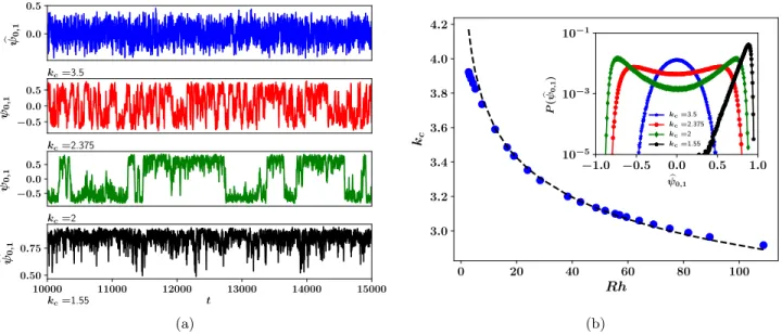
In the turbulent regime Rh still plays the role of the bifurcation parameter but in this case the relevant observables are statistical quantities. In Fig. 2a we show the time series of bψ0,1 and in Fig. 2b their corresponding PDFs for
different values of Rh. At Rh = 3.13, the time series is turbulent with the amplitude of bψ0,1 fluctuating randomly
around the zero mean implying that the symmetry with respect to the centreline is restored for the mode in a statistical sense. The PDF of this time series is close to Gaussian. For Rh = 42.95 we start to see longer duration of time where
b
ψ0,1 has a non-zero amplitude, the corresponding PDF is bimodal with two distinct peaks. This represents the first
bifurcation where the system transitions from a Gaussian distribution to a bimodal distribution with two symmetric maxima. This behaviour is related to the emergence of two symmetric states where the time series is characterised by abrupt and random reversals between these two states. One state is when bψ0,1 > 0 and the other symmetric state is
when bψ0,1 < 0 for long duration. For Rh = 59.45 we get random reversals of the large scale flow with a PDF which is
bimodal with more distinct peaks. As we keep increasing Rh the reversals become rarer until we get to a state where there are no more large scale flow reversals observed indicating another bifurcation. This is seen in the case with Rh = 89.36 where the system was never observed to reverse and the corresponding PDF is unimodal with a non-zero mean. The PDF for the largest Rh = 89.36 chooses either a positive or negative value of bψ0,1 depending on the
initial condition. The unimodal distribution indicates that ensemble averaging is not equivalent to the time averaged system. For each value of Rh examined we have also calculated the corresponding value of kc which is defined by,
kc= (Ω/E)1/2, (6)
where the kinetic energy and the enstrophy are defined respectively, E = h|∇ψ|2iA, Ω = h|∇
2
ψ|2iA, (7)
with the angular brackets h·iA denoting integration over x and y. The value of kc is later used to compare with the
10000 11000 12000 13000 14000 15000 Rh =89.36, kc=2.96 t −0.2 0.0 b ψ0,1 Rh =59.45, kc=3.08 −0.25 0.00 0.25 b ψ0,1 Rh =42.95, kc=3.17 −0.25 0.00 0.25 b ψ0,1 Rh =3.13, kc=3.9 −0.025 0.000 0.025 b ψ0,1 (a) −0.4 −0.3 −0.2 −0.1 0.0 0.1 0.2 0.3 0.4 b ψ0,1 10−4 10−3 10−2 10−1 P ( bψ0 ,1 ) kc=2.96 kc=3.01 kc=3.17 kc=3.9 (b)
FIG. 2: (Color online) (a) Time series of the large scale mode bψ0,1 from the DNS and their corresponding (b) PDFs
for different values of Rh
A similar sequence of bifurcations of the large scale circulation has been observed in laboratory experiments of quasi-2D flow [19] and also in numerical simulations of 2D turbulence [26]. In those studies the boundary conditions were no-slip or free-slip in both x, y boundaries. The energy spectra from our DNS (not shown here) are found to have a peak at an intermediate wavenumber k = 2 when the system displays bimodal behaviour of bψ0,1. Here k =
q k2
x+ k2y
is the amplitude of the wavevector. The 2D turbulent flow is not in the condensate regime where the large scale mode is much larger in amplitude when compared to the rest of the modes. This is in contrast to the study [26] where those DNS spectra peaked at the lowest wavenumber kmin= 1 in the bimodal regime.
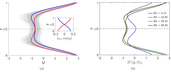
To understand the flow structure in the different regimes we analyse the mean flow profile U (y, t) defined as
U (y, t) = 1 2π
Z 2π 0
u (x, y, t) dx. (8)
Figure 3a illustrates the mean velocity profile for the flow with Rh = 59.45. The blue and red curves represent the mean flow profiles which have been time averaged over the time intervals conditional on bψ0,1 > 0 and bψ0,1 < 0,
respectively. A part of these intervals is shown in the time series for Rh = 59.45 in Fig. 2a. The grey curves indicate the instantaneous realisations of the mean flow profile at different times. The conditionally time-averaged mean flow profiles (blue and red curves in Fig. 3a) are then projected onto the largest mode, which are shown in the inset of Fig. 3a. When bψ0,1 > 0 the conditionally time averaged profile, blue curve in Fig. 3a, shows a stronger westward jet in the
upper half of the domain (π/2 < y < π) than in the lower half (0 < y < π/2). The reverse happens for bψ0,1 < 0 as
seen from the red curve in Fig. 3a. The transition between bψ0,1 > 0 to bψ0,1 < 0 state captures the meandering of the
jets from the upper to the bottom half of the domain. Thus, reversals of the large scale mode leads to modulations or meandering of the jets which occurs on a time scale much longer than the eddy turn over time.
Fig. 3b shows the time averaged mean flow profile hU (y, t)it for four different values of Rh. The lowest value of Rh = 3.13 where the PDF of the large scale mode bψ0,1 is Gaussian shows a mean flow profile which resembles the
forcing. This time averaged profile is symmetric about the centreline y = π/2 while instantaneous profiles break the centreline symmetry. As we increase Rh, in the regime where the PDF of bψ0,1 is bimodal, we see that the
mean flow profile deviates from the form of the forcing and two westward jets develops at the centre. The centreline symmetry is still respected by the time averaged mean flow profile. For the largest value of Rh shown in Fig. 3b which corresponds to a unimodal PDF of bψ0,1, the time averaged mean profile breaks the centreline symmetry. Note that
(a)
-3 -2 -1 0 1 2 3
0 /2
(b)
FIG. 3: (Color online) (a) Conditionally time averaged mean flow profiles when bψ0,1> 0 (blue) and bψ0,1< 0 (red)
for Rh = 59.45. Grey curves represent the instantaneous mean flow profiles. The inset shows the projection of the conditionally time averaged mean flow profiles onto the large scale mode. (b) The time averaged mean flow profiles
hU (y, t)it for four different values of Rh as mentioned in the legend.
IV. MINIMAL MODEL: TRUNCATED EULER EQUATION
Now we seek for a minimal model to capture the dynamics of the random transitions of the large scale flow. To do this we consider the incompressible Euler equation truncated at a maximum wavenumber kmax using a Galerkin
truncation, which in Fourier-Sine basis take the form ∂tψbk=
X
p,q
Ak,p,qψbpψbq (9)
with the interaction coefficients to be given by Ak,p,q=
i 2(q
2
− p2)k−2δkx,px+qx[(pxqy− pyqx)δky,py+qy+ (pxqy+ pyqx)(δky,py−qy − δky,qy−py)], (10)
where δi,j stands for the Kronecker delta. To derive Eqs. (9), (10) one has to replace Eq. (3), the Fourier-Sine
decomposition of ψ(x, y, t), into the governing equation Eq. (1). Taking the inverse Fourier transform of the resulting equation we end up with Eq. (9) and the expression for the interaction coefficients in Eq. (10). This truncated system of ODEs conserves exactly the two quadratic invariants of the Euler Equation (i.e. Eq. (1) with the RHS equal to zero), the kinetic energy E and the enstrophy Ω (see definitions in Eq. (7)).
The fundamental idea of equilibrium statistical mechanics is to construct a probability density on the phase space of a dynamical system based only on the invariants of the dynamics. It is well known [27, 28, 33] that the probability density P( bψk, t) of all the amplitudes of the modes bψkin the N -dimensional phase space of the Euler equation obeys
Liouville’s equation ∂tP + X k ˙ c ψk∂ψbkP = 0, (11)
where the sum here is over all N modes bψk. Here the volume in phase space is conserved by the dynamics according
to Eq. (9) and therefore the microcanonical formalism can be used. In the microcanonical formalism [34], P( bψk, t)
is uniform on all the states with a given set of values for the invariants and vanishes for any other set of values. In our case, if one takes into account only the quadratic invariants of the Euler equation, the microcanonical density is defined as
where bE and bΩ are the energy and enstrophy values at absolute equilibrium [28] and the normalisation factor Z(E, Ω), known as the structure function of the system [34], measures the surface of constant energy and enstrophy over the phase space volume elements dΓ =Qkd bψk. This distribution is appropriate for describing an isolated system of initial
energy E and initial enstrophy Ω, with no exchange with its surroundings, under the assumption that the system exhibits suitable ergodic properties [34].
For the truncated Euler equation (TEE) the control parameter depends only on the initial conditions. The wavenum-ber kc, which is the square root of the ratio of initial enstrophy to initial energy (see Eq. (6)), is taken as the control
parameter for the TEE system. In the full Navier-Stokes equations the equivalent wavenumber is controlled by the friction coefficient (i.e. the value of Rh) when the viscosity is fixed. In Fig. 4b we show the dependence of kc on Rh
for the Navier-Stokes equations and we see that as Rh increases the wavenumber kc decreases like
kc∝ Rh−1/10. (13)
This fit comes from the observation that the energy scales like E ∝ Rh4/5 and the enstrophy scales like Ω ∝ Rh3/5
for the values of Rh in a bigger range than the bimodal regime. So far, we do not have a theoretical explanation for these scalings.
The initial conditions for the TEE are chosen such that kc is as close as possible to the DNS results. We then
integrate Eqs. (9)-(10) using a numerical scheme similar to the one used for the Navier-Stokes equations (see section II). The Fourier amplitudes for the TEE satisfy bψk= 0 for |kx| > kmaxx and |ky| > kmaxy . Note that kmaxx and kymax
are our free parameters for the truncation of the Euler equation. The starting point to obtain a minimal model from the TEE was first to set kxmax= kmaxy = 4, which corresponds to the value of the forcing wavenumber kf we chose
for the Navier-Stokes equations. The basic principle behind this choice is that the dynamics of the large scales, i.e. k < kf, are not affected by viscosity and hence they are governed by the dynamics of the Euler equation as it has
been demonstrated in previous studies [26, 35–37]. We then removed one by one the high wavenumber modes and tried to reproduce the bifurcations as we varied the control parameter kc. Using this procedure we ended up with a
minimal model of 15 complex amplitude modes that captures qualitatively the different bifurcations of bψ0,1 similar
to ones observed in the Navier-Stokes equations. The 15 mode minimal model is composed of the following complex amplitude modes,
b
ψ0,1, bψ0,2, bψ0,3, bψ0,4, bψ1,1, bψ1,2, bψ1,3, bψ1,4, bψ2,1, bψ2,2, bψ2,3, bψ2,4, bψ3,1, bψ3,2, bψ3,3. (14)
Only the positive kx modes are used in the counting of 15 modes, the negative kx modes are directly related by
b
ψ−kx,ky = bψ ∗
kx,ky. A further truncated model of 11 modes could reproduce large scale flow reversals but the solution
starts to depend on the initial conditions. So, we use the 15 mode model to study the bifurcations of the large scale mode bψ0,1.
In Fig. 4a we show the time series of the amplitude of the large scale mode bψ0,1 for different values of kc for the
15 mode minimal model and the inset of Fig. 4b shows the corresponding PDF distributions of the time series. For kc = 3.5 the TEE system exhibits a turbulent time series with a Gaussian PDF. At kc = 2.375 the system shows
abrupt and random reversals of the large scale flow with a bimodal PDF. Thus, when the system transitions from a Gaussian to a bimodal distribution, we observe the first bifurcation over a turbulent background between these two values of kc. As kc decreases, the bimodality in the distribution becomes more pronounced and the reversals
become less frequent. Finally, for kc = 1.55 there is no longer any reversal for the duration of the simulation that
lasted tens of thousands of turnover times. Here, the large scale mode bifurcates to a one-sided unimodal PDF. Clearly this minimal set of ODEs captures the bifurcations between the different turbulent regimes observed in the full Navier-Stokes equations.
In the simulations we observe two different scenarios of emergence and disappearance of large scale flow reversals. At high values of kc(or low Rh values for Navier-Stokes), large scale flow reversals are absent because the time series
are very fluctuating and one can no longer identify the two states. At low kc(or high Rh for Navier-Stokes), mean flow
reversals become less and less probable and eventually are no longer observed in the duration of the simulation. These two scenarios of emergence and disappearance of reversals have also been observed in other contexts [26, 32, 38, 39] and hence we believe that they are generic.
V. LONG-TIME MEMORY AND 1/fα NOISE
A quantity of interest is the mean waiting time τ between successive reversals of bψ0,1 for both the Navier-Stokes
10000 11000 12000 13000 14000 15000 kc=1.55 t 0.50 0.75 b ψ0,1 kc=2 −0.5 0.0 0.5 b ψ0,1 kc=2.375 −0.5 0.0 0.5 b ψ0,1 kc=3.5 0.0 0.5 b ψ0,1 (a) 0 20 40 60 80 100 Rh 3.0 3.2 3.4 3.6 3.8 4.0 4.2 kc −1.0 −0.5 0.0 0.5 1.0 b ψ0,1 10−5 10−3 10−1 P ( b ψ0,1 ) kc=3.5 kc=2.375 kc=2 kc=1.55 (b)
FIG. 4: (Color online) (a) Time series of the large scale mode bψ0,1 for the TEE system. (b) kc= (Ω/E)1/2as a
function of Rh from the DNS. The dashed line is the fit from Eq. (13). Inset: PDFs of the time series of bψ0,1 for the
TEE system. 45 50 55 60 65 70 75 Rh 103 104 τ 1.65 1.70 kc 0 1 2 3 1 / τ ×10−4
FIG. 5: (Color online) Log-linear plot of the mean waiting time τ between successive reversals as a function of Rh in the bimodal regime of the Navier-Stokes equations. Inset: Plot of the mean waiting frequency τ−1 between
successive reversals as a function of kc in the bimodal regime of the TEE.
times. Figure 5 shows τ as a function of Rh for the Navier-Stokes equations and the inset shows how 1/τ varies as a function of kc for the TEE. Figure 5 shows an exponential behaviour, i.e.
log(τ ) ∝ Rh (15)
for the Navier-Stokes equations, while a power-law behaviour τ ∝ (kc− kccrit)
−1 (16)
with a critical wavenumber kcritc ' 1.55 for the minimal model (see inset of Fig. 5). For kc < kccrit =
√ 2 large scale flow reversals are not possible in the TEE minimal model. This can be obtained by expanding the energy and
enstrophy as sums of the Fourier modes, viz. E = h|∇ψ|2i = Nx/2 X kx=−Nx/2 Ny X ky=1 (k2x+ k2y)| bψkx,ky| 2 (17) Ω = h|∇2ψ|2i = Nx/2 X kx=−Nx/2 Ny X ky=1 (k2x+ k 2 y) 2 | bψkx,ky|2 (18)
which in short can be written as E = (| bψ0,1|2+ 2| bψ1,1|2+ ...) and Ω = (| bψ0,1|2+ 4| bψ1,1|2+ ...). Due to conservation
of both energy and enstrophy, kc is always fixed to its initial value. Starting with k2c < 2 with a non-zero initial
value of bψ0,1, if bψ0,1(t) = 0 at some instant t > 0, then Eqs. (17) and (18) imply k2c = Ω/E ≥ 2, which can only
occur if the conservation of energy and enstrophy is broken. This cannot happen in the TEE model, thus for k2 c < 2
the large scale mode satisfies the condition bψ0,1(t) 6= 0 at all times implying no reversal of bψ0,1. In contrast, the
Navier-Stokes equations do not involve conserved quantities that prevent reversals, even for Rh 1. In addition, all the wavenumbers k > kf that are suppressed in the truncated Euler model can act as an additional source of
noise for the Navier-Stokes equations and trigger reversals. We believe that these are the reasons why we observe a different behaviour between the Navier-Stokes equations and the TEE. Note that when we plot τ as a function of kc
for the Navier-Stokes equations we observe τ ∝ exp(k−10c ) (not shown here), which is in agreement with kc∝ Rh−1/10
observed in Fig. 4b. Both the exponential and the power-law behaviour suggest long-term dynamical memory effects of the large scale flow as the bifurcation parameters are varied within the bimodal regimes of the two systems.
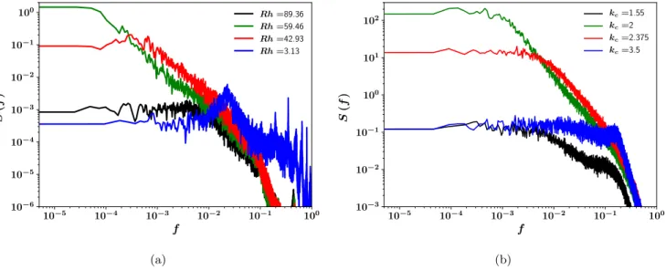
To further support our argument about long-time memory we analyse the spectral properties of the large scale mode b
ψ0,1. In Fig. 6a we plot the power spectra S(f ) for different values of Rh. These spectra were computed from the
time series of the Navier-Stokes equations presented in Fig. 2a. In the Gaussian regime with Rh = 3.13, the spectrum
10−5 10−4 10−3 10−2 10−1 100 f 10−6 10−5 10−4 10−3 10−2 10−1 100 S (f ) Rh =89.36 Rh =59.46 Rh =42.93 Rh =3.13 (a) 10−5 10−4 10−3 10−2 10−1 100 f 10−3 10−2 10−1 100 101 102 S (f ) kc=1.55 kc=2 kc=2.375 kc=3.5 (b)
FIG. 6: (Color online) Power spectra of the large scale mode bψ0,1 for different values (a) of Rh for the Navier-Stokes
equations and (b) of kc for the TEE.
is flat across a large range of frequencies and after a cross-over frequency fc (where S(f ) peaks) it decays. In the
bimodal regime with Rh = 42.93 and Rh = 59.46 the largest part of the frequencies display a power law spectrum S(f ) ∝ 1/fα. As Rh increases within the bimodal regime, the cross-over frequency fc between f0 and 1/fα moves
toward lower frequencies. In other words, the 1/fα range extends to lower frequencies while the f0 range decreases. It is interesting to observe that the level of the power spectrum decays with the observation time similar to studies of other systems that display 1/fα-type noise [40]. Finally, in the unimodal regime with Rh = 89.36 the cross-over
frequency fc between f0 and 1/fα moves to higher frequencies and the amplitude of the f0 part of the spectrum
becomes of the same order with the spectrum for Rh = 3.13 from the Gaussian regime.
Figure 6b on the other hand shows the power spectra from the time series of Fig. 4a, which correspond to different values of kc for the TEE minimal model with 15 modes. The behaviour we just described for the spectra as Rh
increased is reproduced by the TEE minimal model as kc varies from the Gaussian to the bimodal and then to the
unimodal regime (see Fig. 6b).
Understanding of such low frequency noise is of great importance because power spectra of the type
S(f ) ∝ 1/fα (19)
with 0 < α < 2 have been observed in many systems ranging from voltage and current fluctuations in vacuum tubes [41], atmosphere and oceans [42, 43], astrophysical magnetic fields [44] and turbulent flows [38, 39, 45, 46]. These systems often display either fluctuations between symmetric states occurring after random waiting times τ or an intermittent regime with random asymmetric bursts. For this kind of processes, it has been shown that the 1/fα
spectrum is related to a power-law distribution of the waiting time τ of the form
P(τ ) ∝ 1/τβ (20)
with the exponents α and β satisfying the relation α + β = 3 [47]. This relation is valid for random transitions between symmetric states when 0 < α < 2 and 1 < β < 3, and it also holds for random asymmetric bursts when 0 < α < 1 and 2 < β < 3 [38]. We see that the large scale mode bψ0,1 transitions randomly between two symmetric states with
the time average of bψ0,1 being zero in the Gaussian and bimodal regimes. We will thus focus on the case α + β = 3
with 0 < α < 2 and 1 < β < 3.
Now we present a simple argument to show how this relation between the exponents of the distribution and the spectrum emerges. We refer to the following studies where detailed derivations are given [38, 47, 48]. We mention that even though we consider waiting time distributions P (τ ) ∼ τ−β with β > 1, the mean waiting time ¯τ is defined as long as there is an exponential cut-off time scale, see [47, 48]. A typical signal of such a process is shown in Fig. 4a for kc= 2. From the signal of bψ0,1(t) we can obtain the auto-correlation
C(t) = 1 T σ( bψ0,1)2 Z T 0 b ψ0,1(s) bψ0,1(s − t)ds (21)
where T is the total duration of the signal and σ( bψ0,1) is the standard deviation of the signal. Looking at the signal
of bψ0,1(t) (see Fig. 4a) we observe abrupt fluctuations between the states bψ0,1(t) > 0 and bψ0,1(t) < 0, and phases
of long durations τ of bψ0,1(t) with the same sign. Here we assume that the average contributions of short phases do
not contribute to the autocorrelation which allows us to use moving average in order to have cleaner signals. The quantity bψ0,1(s) bψ0,1(s − t) integrated during the long phases contribute a value proportional to τ − t over a length τ
for τ > t and almost zero for τ < t. The time interval s ∈ (0, T ) is then replaced by the variable τ ∈ (t, T ) and the autocorrelation function can be approximated as,
C(t) ≈ 1 T
Z T t
(τ − t)n(τ )dτ for τ t T (22)
where n(τ ) is the number of phases of duration τ . This approximation of the autocorrelation C(t) can be written in terms of the PDF of the waiting times P (τ ) between transitions as
C(t) ≈ 1 τ
Z T
t
(τ − t)P(τ )dτ (23)
because n(τ ) = P(τ )T /τ with T /τ the total number of events. For P(τ ) ∝ 1/τβ we have
C(t) ∝ t−β+2 (24)
with β > 2. Then, using the Wiener-Khinchin theorem we can get the power spectrum S(f ) of bψ0,1 by taking the
Fourier transform of C(t) as T → ∞, which is S(f ) ∝ 1
f3−β
Z ∞ 0
ω−β+2cos(ω)dω (25)
with ω = f t. Thus, the relation between the exponent of the spectrum and the exponent of the PDF of waiting times of transitions between the symmetric states bψ0,1(t) > 0 and bψ0,1(t) < 0 is α = 3 − β.
Figure 7a shows the power spectrum S(f ) of the large scale mode bψ0,1 in the DNS of the Navier-Stokes equations
10−5 10−4 10−3 10−2 10−1 100 f 10−4 10−3 10−2 10−1 100 101 102 103 S (f ) f−1.5 100 101 102 103 τ 10−4 10−3 10−2 10−1 P (τ ) τ−1.5 (a) 10−5 10−4 10−3 10−2 10−1 100 f 10−4 10−3 10−2 10−1 100 101 102 103 S (f ) f−1.5 100 101 102 103 τ 10−4 10−3 10−2 10−1 P (τ ) τ−1.5 (b)
FIG. 7: (Color online) Power spectrum of the large scale mode bψ0,1 from (a) Navier-Stokes equations for Rh = 59.45
and (b) TEE for kc= 2. The insets show the probability density function of the mean waiting time P (τ ) of
successive reversals. The dashed lines show power laws of f−1.5 and τ−1.5 (insets) for comparison.
the DNS shows a range of frequencies where S(f ) has a scaling of f−1.5. We then compare this scaling with the TEE
model and we find here that the scaling is also close to f−1.5. The 1/f1.5 noise is between the well understood white noise with f0 power spectrum and the random walk (Brownian motion) noise with 1/f2 power spectrum. However,
direct differentiation or integration of such convenient signals does not give the required 1/f1.5 spectrum.
The process for generating 1/fα noise here differs strongly from low-dimensional dissipative dynamical systems
because it involves a large number of degrees of freedom with a large network of triads interacting nonlinearly. In addition, 1/fαnoise subsist in the TEE model which represents a system at thermal equilibrium. Our results indicate
that the large scale coherent structures of our turbulent flows are responsible for the long-term dynamical memory of the large scale jets and hence the emergence of the 1/f1.5 noise.
The corresponding PDF of the waiting times P(τ ) are shown as insets in Fig. 7a for the Navier-Stokes equations and in Fig. 7b for the TEE model. Both PDFs show a range of time scales in which a power-law distribution of P(τ ) ∝ τ−1.5compares well with the data. These waiting times, distributed as a power law, reflect the scale invariant
nature of the statistics, and they are associated with the durations spent by the system in the two states. Such heavy-tailed PDFs indicate that long durations have a high probability of occurrence. The scaling of the spectra and of the distribution of the waiting times are in agreement with the relation α + β = 3 both for the Navier-Stokes equations and the mininal TEE model.
VI. CONCLUSION
We have studied in detail the bifurcations of the large scale flow for a turbulent shear flow driven by a Kolmogorov forcing. The domain studied here is anisotropic with an aspect ratio of 2, and so are the boundary conditions that were taken to be free-slip in the spanwise direction, and periodic in the streamwise direction. The geometry and the forcing leads to the formation of jets, with the largest mode in the system bψ0,1 corresponding to two counter
propagating jets. The mode bψ0,1 is not directly excited by the forcing but the energy injected into the forcing scale
is transferred to the largest mode bψ0,1 by an inverse nonlinear transfer. A non-zero value of bψ0,1 does not respect the
centreline symmetry y = πLy/2.
With the friction Reynonds number Rh as the control parameter in the system, we see that the mode bψ0,1 first
displays a Gaussian behaviour in the turbulent regime. Then, as we increase Rh, the large scale mode transitions to a bimodal behaviour denoting the first bifurcation. For larger Rh, we get to another bifurcation with a unimodal distribution where the bψ0,1 mode no longer reverses for the whole duration of the simulation. These bifurcations
of the large scale mode bψ0,1 are related to changes in the form of the time averaged mean flow hU (y, t)it. Similar
of a fully turbulent flow [49]. Using the truncated Euler equation we are able to construct a minimal model, which consists of 15 modes, that effectively captures these bifurcations which occur on top of the turbulent background flow. The control parameter in the TEE model is the ratio of the enstrophy and energy at time t = 0 defined as k2
c = Ω/E.
The role of Rh as the control parameter for the Navier-Stokes equations is now replaced by kc for the TEE model.
We also compared the power spectra from the time series of bψ0,1 and the PDF of the mean waiting times τ
between the two symmetric turbulent states for both the Stokes and the TEE systems. From the Navier-Stokes equations we found the power spectra to scale as S(f ) ∝ 1/f1.5 and the PDFs of the mean waiting times to
obey a power law P(τ ) ∝ 1/τ1.5in the bimodal regime. Moreover, we showed numerically that a minimal TEE model,
which is a system at thermal equilibrium, can qualitatively reproduce these scaling laws for the 1/fα noise and the
PDF of the mean waiting time. This is an interesting result since it has been sometimes believed that 1/fαnoise only occurs in systems out of thermal equilibrium [50]. Although analytical results on TEE exist both on the canonical and microcanonical ensembles, they are limited so far to spatial spectra. It would be of interest to find similar results on temporal spectra or equivalently on correlation functions at different times and to compare them with DNS.
In this paper we have provided a new example where the truncated Euler equations capture the bifurcations of the large scale flow between turbulent states. In this case, the TEE model can capture the bifurcations of the large scale mode even if it is not orders of magnitude above the rest of the modes like in previous studies, a regime where mean field approach or asymptotics might not be applicable. Future studies should aim at understanding whether the TEE model can reproduce transitions of the large scale dynamics in turbulent flows from more realistic models for the dynamics of planetary atmospheres and the ocean, such as advanced quasi-geostrophic and shallow water models.
ACKNOWLEDGEMENTS
The authors would like to thank F. P´etr´elis and V. Shukla for useful discussions in the early stage of this work.
[1] H. A. Dijkstra. Nonlinear climate dynamics. Cambridge University Press, 2013.
[2] M. Ghil. Is our climate stable? bifurcations, transitions and oscillations in climate dynamics. Science for survival and sustainable development, pages 163–184, 2000.
[3] T. F. Stocker, D. Qin, G.-K. Plattner, M. Tignor, S. K. Allen, J. Boschung, A. Nauels, Y. Xia, V. Bex, P. M. Midgley, et al. Climate change 2013: The physical science basis, 2013.
[4] H. Itoh and M. Kimoto. Multiple attractors and chaotic itinerancy in a quasigeostrophic model with realistic topography: Implications for weather regimes and low-frequency variability. J. Atmos. Sci., 53(15):2217–2231, 1996.
[5] M. J. Schmeits and H. A. Dijkstra. Bimodal behavior of the kuroshio and the gulf stream. J. Phys. Oceanogr., 31(12):3435– 3456, 2001.
[6] E. R. Weeks, Y. Tian, J. S. Urbach, K. Ide, H. L. Swinney, and M. Ghil. Transitions between blocked and zonal flows in a rotating annulus with topography. Science, 278(5343):1598–1601, 1997.
[7] B. Semin, N. Garroum, F. P´etr´elis, and S. Fauve. Nonlinear saturation of the large scale flow in a laboratory model of the quasibiennial oscillation. Phys. Rev. Lett., 121:134502, 2018.
[8] A. Renaud, L.-P. Nadeau, and A. Venaille. Periodicity disruption of a model quasibiennial oscillation of equatorial winds. Phys. Rev. Lett., 122(21):214504, 2019.
[9] I Wygnanski, F Champagne, and B Marasli. On the large-scale structures in two-dimensional, small-deficit, turbulent wakes. J. Fluid Mech., 168:31–71, 1986.
[10] O. Cadot, A. Evrard, and L. Pastur. Imperfect supercritical bifurcation in a three-dimensional turbulent wake. Phys. Rev. E, 91:063005, 2015.
[11] M. Breuer and U. Hansen. Turbulent convection in the zero reynolds number limit. EPL (Europhysics Letters), 86:24004, 2009.
[12] R. J. A. M. Stevens, J.-Q. Zhong, H. J. H. Clercx, G. Ahlers, and D. Lohse. Transitions between turbulent states in rotating Rayleigh-B´enard convection. Phys. Rev. Lett., 103:024503, 2009.
[13] Kazuyasu Sugiyama, Rui Ni, Richard J. A. M. Stevens, Tak Shing Chan, Sheng-Qi Zhou, Heng-Dong Xi, Chao Sun, Siegfried Grossmann, Ke-Qing Xia, and Detlef Lohse. Flow reversals in thermally driven turbulence. Phys. Rev. Lett., 105:034503, 2010.
[14] M. Chandra and M. K. Verma. Flow reversals in turbulent convection via vortex reconnections. Phys. Rev. Lett., 110:114503, 2013.
[15] R. Labb´e, J.-F. Pinton, and S. Fauve. Study of the von k´arm´an flow between coaxial corotating disks. Phys. Fluids, 8(4):914–922, 1996.
[16] F. Ravelet, L. Mari´e, A. Chiffaudel, and F. Daviaud. Multistability and memory effect in a highly turbulent flow: Experi-mental evidence for a global bifurcation. Phys. Rev. Lett., 93(16):164501, 2004.
[17] A. de la Torre and J. Burguete. Slow dynamics in a turbulent von K´arm´an swirling flow. Phys. Rev. Lett., 99:054101, 2007.
[18] M. Berhanu, R. Monchaux, S. Fauve, N. Mordant, F. P´etr´elis, A. Chiffaudel, F. Daviaud, B. Dubrulle, L. Mari´e, F. Ravelet, et al. Magnetic field reversals in an experimental turbulent dynamo. Europhys. Lett., 77(5):59001, 2007.
[19] G. Michel, J. Herault, F. P´etr´elis, and S. Fauve. Bifurcations of a large-scale circulation in a quasi-bidimensional turbulent flow. Europhys. Lett., 115(6):64004, 2016.
[20] P. K. Mishra, J. Herault, S. Fauve, and M. K. Verma. Dynamics of reversals and condensates in two-dimensional kolmogorov flows. Phys. Rev. E, 91(5):053005, 2015.
[21] Vladimir Zeitlin. Geophysical fluid dynamics: understanding (almost) everything with rotating shallow water models. Oxford University Press, 2018.
[22] F. Bouchet and E. Simonnet. Random changes of flow topology in two-dimensional and geophysical turbulence. Phys. Rev. Lett., 102(9):094504, 2009.
[23] B. Galperin and P. L. Read. Zonal Jets: Phenomenology, Genesis, and Physics. Cambridge University Press, 2019. [24] F. Bouchet, J. Rolland, and E. Simonnet. Rare event algorithm links transitions in turbulent flows with activated
nucle-ations. Phys. Rev. Lett., 122(7):074502, 2019.
[25] L. P. Kadanoff. Statistical physics: statics, dynamics and renormalization. World Scientific Publishing Company, 2000. [26] V. Shukla, S. Fauve, and M.-E. Brachet. Statistical theory of reversals in two-dimensional confined turbulent flows. Phys.
Rev. E, 94(6):061101, 2016.
[27] R. H. Kraichnan. Inertial ranges in two-dimensional turbulence. Phys. Fluids, 10(7):1417–1423, 1967. [28] R. H. Kraichnan. Statistical dynamics of two-dimensional flow. J. Fluid Mech., 67(1):155–175, 1975.
[29] David Gottlieb and Steven A Orszag. Numerical analysis of spectral methods: theory and applications, volume 26. Siam, 1977.
[30] A. Thess. Instabilities in two-dimensional spatially periodic flows. part i: Kolmogorov flow. Phys. Fluids A, 4(7):1385–1395, 1992.
[31] K. Seshasayanan, V. Dallas, and S. Fauve. Bifurcations of a plane parallel flow with kolmogorov forcing. arXiv preprint arXiv:2004.12418, 2020.
[32] S. Fauve, J. Herault, G. Michel, and F. P´etr´elis. Instabilities on a turbulent background. J. Stat. Mech., 2017(6):064001, 2017.
[33] T. D. Lee. On some statistical properties of hydrodynamical and magneto-hydrodynamical fields. Quart. Appl. Math., 10(1):69–74, 1952.
[34] A. I. Khinchin. Mathematical foundations of statistical mechanics. Dover Publications, 1960.
[35] V. Dallas, S. Fauve, and A. Alexakis. Statistical equilibria of large scales in dissipative hydrodynamic turbulence. Phys. Rev. Lett., 115:204501, 2015.
[36] M. Linkmann and V. Dallas. Large-scale dynamics of magnetic helicity. Phys. Rev. E, 94:053209, 2016.
[37] A. Alexakis and M.-E. Brachet. On the thermal equilibrium state of large-scale flows. J. Fluid Mech., 872:594–625, 2019. [38] J. Herault, F. P´etr´elis, and S. Fauve. 1/fαLow frequency fluctuations in turbulent flows. J. Stat. Phys., 161(6):1379–1389,
2015.
[39] M. Pereira, C. Gissinger, and S. Fauve. 1/f noise and long-term memory of coherent structures in a turbulent shear flow. Phys. Rev. E, 99(2):023106, 2019.
[40] A. Sadegh, E. Barkai, and D. Krapf. 1/f noise for intermittent quantum dots exhibits non-stationarity and critical exponents. New J. Phys., 16(11):113054, 2014.
[41] F. N. Hooge, T. G. M. Kleinpenning, and L. K. J. Vandamme. Experimental studies on 1/f noise. Rep. Prog. Phys., 44(5):479–532, 1981.
[42] K. Fraedrich and R. Blender. Scaling of atmosphere and ocean temperature correlations in observations and climate models. Phys. Rev. Lett., 90:108501, 2003.
[43] A. Costa, A. R. Osborne, D. T. Resio, S. Alessio, E. Chriv`ı, E. Saggese, K. Bellomo, and C. E. Long. Soliton turbulence in shallow water ocean surface waves. Phys. Rev. Lett., 113:108501, 2014.
[44] W. H. Matthaeus and M. L. Goldstein. Low-frequency 1
f noise in the interplanetary magnetic field. Phys. Rev. Lett.,
57:495–498, 1986.
[45] P. Dmitruk and W. H. Matthaeus. Low-frequency 1/f fluctuations in hydrodynamic and magnetohydrodynamic turbulence. Phys. Rev. E, 76:036305, 2007.
[46] P. Dmitruk, P. D. Mininni, A. Pouquet, S. Servidio, and W. H. Matthaeus. Magnetic field reversals and long-time memory in conducting flows. Phys. Rev. E, 90:043010, 2014.
[47] S. B. Lowen and M. C. Teich. Fractal renewal processes generate 1/f noise. Phys. Rev. E, 47:992–1001, 1993.
[48] M. Niemann, H. Kantz, and E. Barkai. Fluctuations of 1/f noise and the low-frequency cutoff paradox. Phys. Rev. Lett., 110(14):140603, 2013.
[49] D. J. Tritton. Physical Fluid Dynamics. Springer Netherlands, 1977. [50] P. Dutta and P. M. Horn. Low-frequency fluctuations in solids: 1