• Aucun résultat trouvé

Stress Testing Engineering: the real risk measurement?

N/A
N/A
Protected

Academic year: 2021

Partager "Stress Testing Engineering: the real risk measurement?"

Copied!
52
0
0

Texte intégral

(1)

HAL Id: halshs-00951593

https://halshs.archives-ouvertes.fr/halshs-00951593

Submitted on 25 Feb 2014

HAL is a multi-disciplinary open access

archive for the deposit and dissemination of sci-entific research documents, whether they are pub-lished or not. The documents may come from teaching and research institutions in France or

L’archive ouverte pluridisciplinaire HAL, est destinée au dépôt et à la diffusion de documents scientifiques de niveau recherche, publiés ou non, émanant des établissements d’enseignement et de recherche français ou étrangers, des laboratoires

Stress Testing Engineering: the real risk measurement?

Dominique Guegan, Bertrand Hassani

To cite this version:

Dominique Guegan, Bertrand Hassani. Stress Testing Engineering: the real risk measurement?. 2014. �halshs-00951593�

(2)

Documents de Travail du

Centre d’Economie de la Sorbonne

Stress Testing Engineering: the real risk measurement?

Dominique G

UEGAN

, Bertrand K. H

ASSANI

(3)

Stress Testing Engineering: the real risk measurement?

February 6, 2014

• Pr. Dr. Dominique Guégan: Université Paris 1 Panthéon-Sorbonne and NYU - Poly, New York, CES UMR 8174, 106 boulevard de l’Hopital 75647 Paris Cedex 13, France, phone: +33144078298, e-mail: dguegan@univ-paris1.fr.

• Dr. Bertrand K. Hassani: Université Paris 1 Panthéon-Sorbonne CES UMR 8174 and Grupo Santander, 106 boulevard de l’Hopital 75647 Paris Cedex 13, France, phone: +44 (0)2070860973, e-mail: bertrand.hassani@santander.co.uk.

Abstract

Stress testing is used to determine the stability or the resilience of a given financial insti-tution by deliberately submitting the subject to intense and particularly adverse conditions which has not been considered a priori. This exercise does not imply that the entity’s failure is imminent, though its purpose is to address and prepare this potential failure. Conse-quently, as the focal point is a concept (Risk) the stress testing is the quintessence of risk management. In this chapter we focus on what may lead a bank to fail and how its resilience can be measured. Two families of triggers are analysed: the first stands in the impact of external (and/or extreme) events, the second one stands on the impacts of the choice of inadequate models for predictions or risks measurement; more precisely on models becoming inadequate with time because of not being sufficiently flexible to adapt themselves to dy-namical changes. The first trigger needs to take into account fundamental macro-economic data or massive operational risks while the second trigger deals with the limitations of the quantitative models for forecasting, pricing, evaluating capital or managing the risks. It may be argued that if - inside the banks - limitations, pitfalls and other drawbacks of mod-els used were correctly identified, understood and handled, and if the associated products were correctly known, priced and insured, then the effects of the crisis may not have had so important impacts on the real economy. In other words, the appropriate model should be

(4)

able to capture real risks (including in particular extreme events) at any point in time, or ultimately a model management strategy should be considered to switch from a model to another during extreme market conditions.

1

Introduction

Stress testing (Berkowitz (1999), Quagliariello (2009), Siddique and Hasan (2013)) is used to determine the stability or the resilience of a given financial institution by deliberately submitting the subject to intense and particularly adverse conditions which has not been considered a priori. This involves testing beyond the traditional capabilities - usually to determine limits - to confirm that intended specifications are both accurate and being met in order to understand the process underlying failures. This exercise does not mean that the entity’s failure is imminent, though its purpose is to address and prepare this potential failure. Consequently the stress testing is the quintessence of risk management.

Since the 1990’s most financial institutions have conducted stress testing exercises on their bal-ance sheet, but it is only in 2007 following the current crisis, that regulatory institutions became

interested in analyzing and measuring the resilience of financial institutions1in case of dramatic

movements of economic fundamentals such as the GDP. Then, stress tests have been regularly performed by regulators to insure that banks are properly adopting practices and strategies which decrease the chance of a bank failing, in turn jeopardising the entire economy (Berkowitz (1999)).

Originally governments and regulators were keen on measuring financial institutions’ resilience -and by extension the entire system - in order to avoid future failure that ultimately the tax payer would have to support. The stress testing framework engenders the following questions: if a risk is identified even with the smallest probability of occurrence why is it not directly integrated in the traditional risk models? Why should we have two processes addressing the same risks, the first under “normal” conditions and the second under stressed condition knowing that the risk universe combine them? Therefore, are the stress tests really discussing the impact of an exogenous event on a balance sheet or of an endogenous failing process, for instance when a

1

In October 2012, U.S. regulators unveiled new rules expanding this practice by requiring the largest American banks to undergo stress tests twice per year, once internally and once conducted by the regulators.

(5)

model is unable to capture certain risks. In other words is the risk of failing and threatening the entire system only exogenous?

As the ultimate objective is the protection of the system, a clear definition of the latter is neces-sary as soon as in the capitalist world banks are the corner stone. Figure 1 exhibits a simplified version of the banking system used in most developed countries around the globe. It has three layers, the "real" economy at the bottom, the interbanking market in the middle and the central bank at the top. Based on this representation if we want to measure the system resilience we need to identify what may potentially threaten the system. Here, we may reasonably assume that stress-testing and systemic-risk measurement are ultimately connected. As discussed below a bank may either fail because of a lack of capital or a lack of liquidity. Regarding this risk of illiquidity we would like to illustrate how tricky it may be to cope with such a risk. In fact, a bank balance sheet is fairly simple assets are composed of intangible assets, investments and lendings while the liabilities are on the top shareholder’s equity and subordinated debt then comes the wholesale funding and finally clients deposits. By changing the money with a short duration, such as savings into money with a longer one through lending, a bank is operating a maturity transformation. This ends up in banks having an unfavorable liquidity position as they do not have access to the money they lent while the money they owe to customer can be

withdrawn at any time on demand. Through ALM2 banks are managing this mismatch, and we

cannot emphasize enough this point implying that banks are structurally illiquid.

Regarding our simplistic representation of the financial system, figure 1 exhibits four potential failure spots: (i) The central bank cannot provide any liquidity anymore; (ii) Banks are not funding each other anymore; (iii) A bank of sensible size is failing; (iv) The banks stop financing the economy.

Regarding the first point (i), considering that the purpose of a central bank is refinancing loans provided by commercial banks controlling inflation, unemployment rate, etc. , as soon as this central bank ceases functioning properly the entire system collapses (uncontrolled inflation, etc.). This point discusses a model failure and falls beyond the stress-testing exercise. Some examples

2

(6)

Figure 1: Financial System

may be found in the Argentinian or the Russian central banks failure in the 1990’s. Considering the second point (ii), if banks are not funding each other then some will face a tremendous lack of liquidity or confidence intra-bank and may fail (for instance it was the case when banks refused to help Lehman Brothers the 15th September 2007). In this case we are addressing the way financial institutions face the risk of illiquidity. On the third point (iii), a bank may fail due to a lack of capital. Consequently how a bank is supposed to be evaluating its capital requirement considering the major risks is crucial. In 2008 the insurance company AIG almost failed due to a lack of capital when most of the CDS they sold had been triggered simultaneously. This is the backbone of risk management inside a bank. Regarding the last point (iv), and assuming that ultimately the purpose of banks is to generate a profit financing the real economy it is highly unlikely that they would do it in case of high stress. A lack of liquidity may lead a bank to stop funding the economy and by the way may engender corporate and retail defaults. These defaults in chain may themselves drive the financial institution to bankruptcy. In that latter case we are clearly discussing the way banks are addressing the credit risk.

(7)

Whatever the origin of the stress inside the banks a failure causes important damages: bankruptcy, alteration of confidence on the markets and between the banks, recession in the real economy, succession of defaults from the enterprises, lack of liquidity and claiming of credits. The global banking system can be strongly and irreparably disrupted. The idea underlying the stress tests is to imagine the scenarii illustrating the previous situations to introduce dynamical solutions which can avoid, at each time any dramatic failures.

In this chapter we focus on what may lead a bank to fail and how its resilience can be measured. As the system is as strong as its weakest link large enough to trigger a chain reaction, by measur-ing the resilience of all the banks simultaneously, the resilience of the entire system is assessed. The right question is what may trigger this chain reaction. Following Lorenz (Lorenz (2010)) we have to capture the butterfly which may engender a twister? In this chapter two families of triggers are analysed: the first stands in the impact of external (and/or extreme) events, the second one stands on the impacts of the choice of inadequate models for predictions or risks measurement; more precisely on models becoming inadequate with time because of not being sufficiently flexible to adapt themselves to dynamical changes. The first trigger needs to take into account fundamental macro-economic data or massive operational risks while the second trigger deals with the limitations of the quantitative models for forecasting, pricing, evaluating capital or managing the risks. An example of model originating of a system failure was the use of the Gaussian copula to price CDOs (and CDS) as mis-capturing the intrinsic upper tail dependen-cies characterizing CDOs tranches correlations mechanically ledding to mis-price and mis-hedge positions and as a matter of fact producing the experienced cataclysm. It may be argued that if - inside the banks - limitations, pitfalls and other drawbacks of models used were correctly iden-tified, understood and handled, and if the associated products were correctly known, priced and insured, then the effects of the crisis may not have had so important impacts on the real economy.

This chapter is structured as follows. In Section two the stress testing framework is presented. In the third Section the mathematical tools required to develop the stress testing procedures are introduced. Finally, in a fourth section we discuss and illustrate integration of the stress-testing strategy directly into the risk models.

(8)

2

The stress-testing framework

A stress-testing exercise means choosing scenarii that are costly and rare which can lead to the financial institution failure, Thus we need to integrate them into a model in order to measure their impact. The integration process may be a simple linear increasing of parameters to enlarge the confidence interval of the outcomes, or switch to a more advanced model predicting the po-tential loss due to an extreme event or a succession of extreme events by implementing various methodologies allowing the capture of multiple behaviours, or adding exogenous variables.

The objective of this exercise is to strengthen the framework for the risk management by under-standing extreme exposures, i.e. exposure that may fall beyond the “business as usual” capture domain of a model. We define the capture domain of a model by its capability to be resilient to the occurrence of an extreme event, i.e. the pertaining risk measure would not fluctuate or only in a narrow range of values, or would not breach the selected confidence intervals too many times.

By stressing a value the financial institution naturally acknowledges the fact that their models and the resulting measurements are reflecting their exposure only up to a certain extent. As a matter of fact this is due to data sets on which the models are calibrated that are not containing the entire information or are not adapted to the evolution of the real world. Indeed, the data set only contains past incidents, and even if crisis outcomes are integrated it does not integrate the future extreme events which are by definition unknown. In other words, even if the models are conservative enough to consider eventual Black Swans (Taleb (2010)) the stress-testing enables envisaging Black Swans with blue eyes and white teeth.

Selecting the appropriate scenario is equivalent to selecting the factors that may have an impact on the models, (e.g. covariates) and to define the level of stress. These scenarii are supposed to characterise shocks likely to occur more than what historical observations say: shocks that have never occurred (stress expected loss), shocks reflecting circumstantial break downs, shocks reflecting future structural breaks. Mathematically all new categories of shocks entail drawing

from some new factor distribution fwhich is not equal to the original distribution f

(9)

and specific events, such as crash, bankrupt, systemic failure, etc.

When scenarii are assessed, practitioners have to check the various outcomes. Are they relevant for the goal? Are they internally consistent? Are they archetypal? Do they represent relatively stable outcome situations? The risk managers should identify the extremes of the possible outcomes of the driving forces and check the dimensions for consistency and plausibility. Almost three key points should be addressed:

1. The time frame: are the "new" trends compatible within the time frame in question? 2. The internal consistency: do the forces describe uncertainties that can construct probable

scenarii?

3. The stakeholder influence: Is it possible to create reliable scenarii considering a potential negative influence from the stakeholders?

Now, there are a lot of sources which need to be taken into account inside stress tests. We enu-merate the risks for which a particular attention must be constantly renewed information must be continuously updated and potential severe outcome reflected in banks’ internal assessments. These risks are mainly market, credit, operational and liquidity risks.

Applied to market risk some procedures have traditionally been applied to banks’ trading portfo-lios by considering multiple states of nature scenarii impacting various risk factors. Traditionally three kinds of approaches are used, standard scenarii, historical scenarii and worst-case scenarii. This type of stress testing is probably the simplest and therefore suffers from the limitations related to over simplicity.

As being the fundamental activity of a bank credit risk stress testing is much wider and has even been integrated into the capital calculations formulas through the Loss Given Default (LGD) done by financial institutions. But approaches are not limited to capital calculations as stress testing is also interesting for more traditional credit risk measure. For example Majnoni et al. (2001) linked the ratio non-performing loan over total assets to several fundamentals macroeco-nomic variables such as nominal interest rates, inflation, GDP, etc.; Bunn et al. (2005) measured the impact of aggregate default rates and LGD evaluation of aggregated write-offs for corporate

(10)

mortgages and unsecured lendings using standard macroeconomic factors like GDP, unemploy-ment, interest rates, income gearing and loan to value ratios. This last component may be particularly judicious in the UK considering the level of interest rate for mortgages sold in the past few years. Practitioners (Pesola (2007)) argue that unexpected shocks should drive loans related losses and the state of system, i.e. a more fragile system would worsen the losses. There-fore factors weakening a financial system should interact in a multiplicative way. Counterparty credit exposure may either be represented by the “current” exposure, the “expected” exposure or the “expected positive” exposures. Stressing the exposure distributions would naturally im-pact the measures based on them, for instance the Credit Value Adjustement (CVA) (Gregory (2012)) via the expected exposure or the expected loss via the expected positive exposure.

By using extreme scenarii operational risks measurement are naturally stressed. Besides as the methodologies implemented are expected by the regulator to be conservative, i.e. to provide risk measures larger than what empirical data or traditional approach would give to practitioners. However these are not sufficient to provide an accurate representation of the risks over time. Alternative strategies need to be developed such as those presented in the next section.

Liquidity risk arises from situations in which an entity interested in trading an asset cannot do it because nobody wants to buy or sell it with respect to the market conditions. Liquidity risk becomes particularly important to entities which currently hold an asset (or want to held it) since it affects their capability to trade. Manifestations of liquidity risk are very different if it comes from price droping to zero. In case an asset’s price falling to zero the market is saying that the asset is worthless. However if one bank cannot find a counterparty interested in trading the asset this may only be a problem of market equilibrium, i.e. the participants have trouble finding each other. This is why liquidity risk is usually found to be higher in emerging or low-volume markets. Accordingly liquidity risk has to be managed in addition to market, credit and operational risks. Because of its tendency to compound other exposures it is difficult or impossible to isolate liquidity risk. Some ALM techniques can be applied to assessing liquidity risk. A simple test for liquidity risk is to look at future net cash flows on a day-by-day basis where any day that has a sizeable negative net cash flow is of concern. Such an analysis can be supplemented with stress testing.

(11)

In this chapter we only partially deal with the “micro” liquidity risk, i.e. the liquidity of an asset, by opposition to the “macro” liquidity exposure, i.e. of a financial institution which is an aggregated measure assuming that it is included in market prices dropping up to a certain extent which is captured in the market risk measurement. The liquidity position of a financial institution is measured by the quantity of assets to be sold immediately to face the liquidity requirements, even considering a haircut, while the price of an asset on the market is illiquid if there is no demand and its price is actually equal to 0, and consequently the measure should be forward. As a result considering the previous statement - in the next section - we focus on methodologies to measure and stress the solvency of financial institutions in relation to market, credit and operational risks.

3

Tools

In this section some of the tools required to develop stress test strategies are introduced. The main ingredient which is determinant in our point of view is the information set on which our work relies. This set is definitively determinant and whatever the methodologies we will use latter the conclusions cannot be done without referring to this information set. After discussing the role of the data set we briefly recall the measures of risks which can be used and how they can be computed. This leads us in a first step to introduce the distributions appearing relevant to obtained realistic risks measures (from an univariate point of view) and second the notion of dependence permitting to capture interdependences between the risks in order to properly evaluate their risk measures in a multivariate framework. Finally the question of dynamics that should be captured in all strategies of risk management is also discussed.

An a priori which is important to note is that financial data sets are always formed with discrete time data and they cannot be directly associated to continuous data thus in this chapter the techniques we present are adapted to this kind of data set.

(12)

3.1 Data mining

Feeding the scenario analysis and evaluating the potential outcomes lie on the quality of the information set used. Therefore a data mining process should be undertaken. Data mining is the computational process of discovering patterns in large data sets. The objective process is to extract information from a data set, make it understandable and prepare it for further use. In our case the data mining step is equivalent to a pre-processing exercise. Data mining involves almost six common classes of tasks (Fayyad et al. (1996)):

1. Anomaly detection – This is the search of events which do not conform to expected pat-terns. These anomalies are often translated into actionable information.

2. Dependency analysis – The objective is to detect interesting relationships between variables in databases.

3. Clustering – Cluster analysis consists in the task of creating groupings of similar objects. 4. Classification – The classification consists in generalizing known structure to be applicable

to new data sets.

5. Regression & fittings – This statistical process purpose is to find the appropriate model, distribution or function which represent the "best" (in a certain sense) fit for the data set. 6. Summarisation – This step purpose is to provide a synthetic representation of the data

set.

These classical techniques are recalled as they could be interesting in certain cases to determine the sets or subsets on which we should work. They could also be useful to exhibit the main features of the data before beginning a probabilistic analysis (for the risk measure) or doing a time series analysis to examine the dynamics which seems the more appropriate for stress testing purposes.

3.2 Risk measures

Even if at the beginning the risk in the banks was evaluated using the standard deviation applied to different portfolios the financial industry uses now the quantile-based downside risk measures

(13)

measures the losses that may be expected for a given probability, and corresponds to the quan-tile of the distribution which characterizes the asset or the type of events for which the risk has to be measured. Thus, the fit of an adequate distribution to the risk factor is definitively an important task to obtain a reliable value of the risk. Then, in order to measure the importance of the losses beyond the VaR percentile and to capture the diversification benefits the expected shortfall measure has been introduced.

The definitions of these two risks measures are recalled below:

Definition 3.1. Given a confidence level α ∈ (0, 1), the V aRα is the relevant quantile3 of the

loss distribution, V aRα(X) = inf{x | P [X > x] 6 1 − α} = inf{x | FX(x) > α} where X is a

risk factor admitting a loss distribution FX .

Definition 3.2. The Expected Shortfall (ESα) is defined as the average of all losses which are

equal or greater than V aRα :

ESα(X) = 1

1 − α

Z 1

α V aRαdp

The Value at Risk initially used to measure financial institutions market risk was popularised by Riskmetrics (1993). This measure indicates the maximum probable loss given a confidence

level and a time horizon. The V aRα is sometimes referred as the “unexpected” loss. The

ex-pected shortfall has a number of advantages over the V aRα because it takes into account the

tail risk and fulfills the sub-additive property. It has been widely dealt with in the literature, for instance in Artzner et al. (1999), Rockafellar and Uryasev (2000; 2002) and Delbaen (2000).

Relationships between V aRα and ESα, for some distributions can be found in this book inside

the chapter of Guégan et al. (2014).

Nevertheless even if the regulators asked to the banks to use the V aRα and recently the ESα to

measure their risks and ultimately provide the capital requirements to avoid bankruptcy these risk measures are not entirely satisfactory:

• They provide a risk measure for an α which is too restrictive considering the risk associated to the various financial products;

3

V aRα(X) = q1−α= F− 1

(14)

• The fit of the distribution functions can be complex or inadequate in particular for the practitioners who want to follow the guidelines proposed by the regulators (Basel II/III guidelines). Indeed, in case of the operational risks the suggestions is to fit a GPD which does not correspond very often to a good fit and whose carrying out can be difficult. • It may be quite challenging to capture extreme events. Taking into account these events

in modelling the tails of the distributions is determinant.

• Finally all the risks are computed considering unimodal distributions which can be non realistic in practice.

Recently several extensions have been analysed to overcome these limitations and to propose new routes for the risk measures. These new techniques are briefly recalled and we suggest the reader to look at the chapter of Guégan et al. (2014) in this book for more details, developments and applications:

• Following our proposal we suggest the practitioners to use several α to obtain a spectrum of their expected shortfall and to visualize the evolution of the ES with respect to these different values. Then, a unique measure can be provided making a convex combination of these different ES with appropriate weights. This measure is called spectral measure (Acerbi and Tasche (2002)).

• In the univariate approach if we want to take into account information contained in the tails we cannot restrict to the GPD as suggested in the guidelines provided by the regu-lators. There exist other classes of distributions which are very interesting, for instance the generalized hyperbolic distribution (Barndorff-Nielsen and Halgreen (1977)), the ex-treme value distributions including the Gumbel, the Frechet and the Weibull distributions (Leadbetter (1983)), the α-stable distributions (Taqqu and Samorodnisky (1994)) or the

g-and-h distributions (Huggenberger and Klett (2009)) among others.

• Nevertheless the previous distributions are not always sufficient to properly fit the infor-mation in the tails and another approach could be to build new distributions shifting the original distribution on the right or left parts in order to take a different information in the tails. Wang (2000) proposes such a transformation of the initial distribution which provides a new symmetrical distribution. Sereda et al. (2010) extend this approach to

(15)

distinguish the right and left part of the distribution taking into account more extreme events. The function applied to the initial distribution for shifting is called a distortion function. This idea is ingenious as the information in the tails is captured in a different way that using the previous classes of distributions.

• Nevertheless when the distribution is shifted with a function close to the Gaussian one as in Wang (2000) and Sereda et al. (2010) the shift distribution remains unimodal. Thus we propose to distort the initial distribution with polynomials of odd degree in order to create several humps in the distributions. This permits to catch all the information in the extremes of the distributions, and to introduce a new coherent risk measure ρ(X)

computed under the g ⊗ FX distribution where g is the distortion operator and FX the

initial distribution, thus we get:

ρ(X) = Eg[FX−1(x)|FX−1(x) > FX−1(δ)]. (3.1)

All these previous risk measures can be included within a stress testing strategy.

3.3 Univariate distributions

This section proposes several alternatives for the fitting of a proper distribution to the infor-mation set related to a risk (losses, scenarios, etc.). The knowledge of the distributions which characterises each risk factor is determinant for the computation of the associated measures and will be also determinant in the case of a stress test. The elliptical domain needs to be left aside to consider distributions which are asymmetric and leptokurtic like the Generalized Hyperbolic distributions, Generalized Pareto distributions, or Extreme Value Distributions among others. Their expressions are recalled in the following.

The Generalized Hyperbolic Distribution (GHD) is a continuous probability distribution defined as a mixture of an inverse Gaussian distribution and a normal distribution. The density function associated to the GHD is:

f (x, θ) = (γ/δ) λ2πKλ(δγ) eβ(x−µ)Kλ−1/2(α p δ2+ (x − µ)2) (p δ2+ (x − µ2)/α)1/2−λ , (3.2)

with 0 ≤ |β| < α. This class of distributions is very interesting as it relies on five parameters. If the shape parameter λ is fixed then several well known distributions can be distinguished:

(16)

1. λ = 1: hyperbolic distribution 2. λ = −1/2: NIG distribution

3. λ = 1 and ξ → 0: Normal distribution

4. λ = 1 and ξ → 1: Symmetric and asymmetric Laplace distribution 5. λ = 1 and χ → ±ξ: Inverse Gaussian distribution

6. λ = 1 and |χ| → 1: Exponential distribution 7. −∞ < λ < −2: Asymmetric Student

8. −∞ < λ < −2 and β = 0: Symmetric Student

9. γ = 0 and 0 < λ < ∞: Asymmetric Normal Gamma distribution

The four other parameters can be then associated to the first four moments permitting a very good fit of the distributions to the corresponding losses.

Another class of distributions is the Extreme Value Distributions built on sequences of maxima obtained from the initial data sets. To introduce this class, the famous Fisher-Tippett theorem needs to be recalled:

Theorem 3.1. Let be (Xn)a sequence of i.i.d.r.v. If it exists constants cn > 0, dn ∈ IR and a

non degenerated distribution function Gα such that

c−1n (Mn− dn)→ GL α (3.3)

then Gα is equal to:

Gα(x) =      exp(−(1 + αx)α1) α 6= 0, 1 + αx > 0 exp(−e−x) α = 0, x ∈ IR

This function Gα(x) contains several classes of extreme values distributions:

. Fréchet (type III) : Φα(x) = G1/α(x−11/α) =      0 x ≤ 0 exp(−x−α), x > 0, α > 0 . Weibull (Type II) : Ψα(x) = G−1/α(x+11/α) =

     exp{−(−xα)}, x ≤ 0, α > 0 1

(17)

. Gumbel (Type I) : Λ(x) = G0(x) = exp(−e−x), x ∈ IR.

Considering only the maxima of a data set is an alternative to model in a robust way the impact of the extremes of a series within a stress testing strategy.

Another class of distributions permitting to model the extremes is the distribution built on a data set defined above or under a threshold. Let X a r.v. with distribution function F and right

end point xF and a fixed u < xF. Then,

Fu(x) = P [X − u ≤ x|X > u], x ≥ 0,

is the excess distribution function of the r.v. X (with the df F ) over the threshold u, and the function

e(u) = E[X − u|X > u]

is called the mean excess function of X which can play a fundamental role in risk management.

The limit of the excess distribution has the distribution Gξ defined by:

Gξ(x) =      1 − (1 + ξx)− 1 ξ ξ 6= 0, 1 − e−x ξ = 0, . where, x ≥ 0 ξ ≥ 0, 0 ≤ x ≤ −1ξ ξ < 0, .

The function Gξ(x) is the standard Generalized Pareto Distribution. One can introduce the

related location-scale family Gξ,ν,β(x) by replacing the argument x by (x − ν)/β for ν ∈ IR,

β > 0. The support has to be adjusted accordingly. We refer to Gξ,ν,β(x) as GPD.

Another class of distributions is the class of α-stable distributions defined through their chara-teristic function also relying on several parameters. For 0 < α ≤ 2, σ > 0, β ∈ [−1, 1] and

µ ∈ R+, S

α(σ, β, µ) denotes the stable distribution with the characteristic exponent (index of

stability) α, the scale parameter σ, the symmetric index (skewness parameter) β and the location

parameter µ. Sα(σ, β, µ) is the distribution of a r.v. X with characteristic function,

E[eixX] =      exp(iµx − σα|x|α(1 − iβsign(x)tan(πα/2))) α 6= 1, exp(iµx − σ|x|(1 + (2/π)iβsign(x)ln|x|)) α = 1 ,

(18)

where x ∈ R, i2 = −1, sign(x) is the sign of x defined by sign(x) = 1 if x > 0, sign(0) = 0 and sign(x) = −1 otherwise. A closed form expression for the density f(x) of the distribution

Sα(σ, β, µ) is available in the following cases: α = 2 (Gaussian distribution), α = 1 and β = 0

(Cauchy distribution) and α = 1/2 and β = +/ − 1 (Levy distributions). The index of stability

α characterises the heaviness of the stable distribution Sα(σ, β, µ).

Finally we introduce the g-and-h random variable Xg,h obtained transforming the standard

normal random variable with the transformation function Tg,h:

Tg,h(y) =      exp(gy)−1 g exp( hy2 2 ) g 6= 0, yexp(hy22) g = 0, . Thus Xg,h= Tg,h(Y ), when Y ∼ N(0, 1).

This transformation allows for asymmetry and heavy tails. The parameter g determines the di-rection and the amount of asymmetry. A positive value of g corresponds to a positive skewness. The special symmetric case which is obtained for g = 0 is known as h distribution. For h > 0 the distribution is leptokurtic with the mass is the tails increasing in h.

Thus to model the margins of all items forming a portfolio we have several choices in order to capture asymmetry, leptokurtosis and extreme events:

• The Generalized Hyperbolic Distribution

• The Extreme Value Distribution Gα, α ∈ IR which describes the limit distributions of

normalised maxima

• The Generalized Pareto Distribution Gξ,β(x), ξ ∈ IR, β > 0 which appears as the limit

distribution of scaled excesses over high thresholds. • The α-stable distributions

(19)

Now with respect to the risks we need to measure the estimation and the fitting of the univariate distributions will be adapted to the data sets. The models will be different depending on the kind of risks we would like to investigate.

3.4 Interdependence between risks

A necessity of the stress testing is to take into account the interactions or interdependences be-tween the entities, business units, items or risks. In most of the case, a bank will be associated to a unique risk portfolio and this one is often modelled as a weighted sum of all its parties. This approach is very restrictive as even if it captures in a certain sense the correlation between the lines it is not sufficient to model all the dependences between the risks characterising the bank. The same observation can be done when we consider the interactions between the different banks trading by the way the same products. We need to bypass this univariate approach and work with a multivariate approach. This multivariate approach permits to explain and measure the contagion effects between all the parties to model the systemic risks and their possible propaga-tion between the different parties.

A robust way to measure the dependence between large data sets is to compute their joint distri-bution function. As soon as independence between the assets or risks characterizing the banks or between the banks cannot be assumed measuring interdependence can be done through the notion of copula. Recall that a copula is a multivariate distribution function linking a large set of data through their standard uniform marginal distributions (Bedford and Cooke (2001), Berg and Aas (2009)). In the literature, it has often been mentioned that the use of copulas is difficult when we have more than two risks apart from using elliptical copulas such as the Gaussian one or the Student one (Gourier et al. (2009)). It is now well known that these restrictions can be released considering recent developments on copulas either using nested copulas (Sklar (1959), Joe (2005)) or vine copulas (Mendes et al. (2007), Rodriguez (2007), Weiss (2010), Brechmann et al. (2010), Guégan and Maugis (2010) and Dissmann et al. (2011)). These n-dimensional copulas need to be fed by some marginal distributions. For instance they can correspond to distributions characterizing the various risks faced by a financial institution. The calibration of the exposure distribution plays an important role in the assessment of the risks, whatever the method used for the dependence structure as discussed in the next section.

(20)

Until now most practitioners use Gaussian or Student t-copulas however they fail to capture asymmetric (and extreme) shocks (for example operational risks severity distributions are

asym-metric - sic!). Using a Student t-copula with three degrees of freedom4 to capture a dependence

between the largest losses would mechanically imply a higher correlation between the very small losses. An alternative is to use Archimedean or Extreme Value copulas (Joe (1997a)) which have attracted particular interest due to their capability to capture the dependence embedded in different parts of the marginal distributions (right tail, left tail and body). The mechanism is recalled in the following.

Let X = [X1, X2, ..., Xn] be a vector of random variables, with joint distribution F and marginal

distributions F1, F2, ..., Fn . Sklar (1959) theorem insures the existence of a function C(.)

map-ping the individual distribution to the joint distribution:

F (x) = C(F1(x1), F2(x2), ..., Fn(xn)).

From any multivariate distribution F , the marginal distributions Fi can be extracted, and also

the copula C. Given any set of marginal distributions (F1, F2, ..., Fn) and any copula C the above

formula can be used to compute the joint distribution with the specified marginals and copula. The function C can be an Elliptical copula (Gaussian and Student Copulas) or an Archimedean copulas (defined through a generator) as

C(FX, FY) = φ−1[φ(FX) + φ(FY)],

including the Gumbel, the Clayton the Franck copulas, among others. The Archimedean copula are easy to use because of the link existing between the Kendall’s tau and the generator φ:

τ (Cα) = 1 + 4 Z 1 0 φα(t) φα(t) dt. (3.4)

If we want to measure the interdependence between more than two risks the Archimedean nested copula is the most intuitive way to build n-variate copulas with bivariate copulas and consists in composing copulas together yielding formulas of the following type. For instance when n = 3:

F (x1, x2, x3) = Cθ12(F (x1), F (x2), F (x3))

= Cθ1(Cθ2(F (x1), F (x2)), F (x3)) 4

(21)

where θi, i = 1, 2 is the parameter of the copula. This decomposition can be done several times,

allowing to build copulas of any dimension under specific constraints to insure that it is always a copula. Therefore a large number of multivariate Archimedean structures have been developed for instance, the fully nested structures, the partially nested copulas and the hierarchical ones. Nevertheless all these architectures imply restrictions on the parameters and impose using an Archimedean copula at each node, making their use limited in practice. To bypass the restric-tions imposed by the previous nested strategy an intuitive approach proposed by Genest et al. (1995) can be used based on a pair-copula decomposition such as the D-vine (Joe (1997b)) or the R-vine (Mendes et al. (2007)). These approaches rewrite the n-density function associated with the n-copula as a product of conditional marginal and copula densities. All the conditioning pair densities are built iteratively to obtain the final one representing the entire dependence structure. The approach is simple and has no restriction for the choice of functions and their parameters. Its only limitation is the number of decompositions to consider as the number of vines grows exponentially with the dimension of the data sample and thus requires the user to

select a vine from n!2 possible vines, Capéraà et al. (2000), Galambos (1978), Brechmann et al.

(2010) and Guégan and Maugis (2010; 2011). These are briefly introduced now.

If f denotes the density function associated with the distribution F of a set of n r.v.X, then the joint n-variate density can be obtained as a product of conditional densities. For instance when

n = 3 the following decomposition is obtained:

f (x1, x2, x3) = f (x1).f (x2|x1).f (x3|x1, x2),

where,

f (x2|x1) = c1,2(F (x1), F (x2)).f (x2),

and c1,2(F (x1), F (x2)) is the density copula associated with the copula C which links the two

margins F (x1) and F (x2). With the same notations we have:

f (x3|x1, x2) = c2,3|1(F (x2|x1), F (x3|x1)).f (x3|x1)

(22)

Then,

f (x1, x2, x3) =f (x1).f (x2).f (x3)

.c1,2(F (x1), F (x2)).c1,3(F (x1), F (x3))

.c2,3|1(F (x2|x1), F (x3|x1)).

(3.5)

Other decompositions are possible using different permutations. These decompositions can be used whatever the links between the r.v. as there is no constraint. To use it in practice and eventually to obtain an initial measure of dependence between the risks inside the banks the first conditioning has to be selected.

3.5 Dynamic approach

In order to take into account events at the origin of stress some banks consider them as single events by simply summing them thus the complete dependence scheme including their arrival time is not taken into account; it appears unrealistic as it may lead to both inaccurate capital charge evaluation and wrong management decisions. In order to overcome the problems created by these choices we suggest to use the following methodology based on the existence of depen-dencies between the losses through a time series process.

The dependence between assets, risks, etc. within a bank and with other banks exists and it is crucial to measure it. We propopse in the previous subsection a way to take them into account. If it does correctly it can avoid the creation of systemic risks. Nevertheless sometimes this dependence does not appear and it seems that the independence assumption cannot be rejected a

priori, thus a profound analysis should always be performed at each step of the cognitive process.

Therefore, in order to build a model close to the reality, static models have to be avoided and intrinsic dynamics should be introduced. The knowledge of this dynamical component should allow to build robust stress tests. To avoid bankruptcies and failures, generally we focus on the incidents performing any probabilistic study as proposed in the previous subsections nevertheless analysing the dynamics embedded within the incidents through time series will permit to be more

reactive and close to the reality. If (Xt)t ∀t denotes the losses, then our objective is to propose

(23)

in the formal following way:

Xt= f (Xt−1,...) + εt, (3.6)

where the function f (.) can take various expressions to model the serial correlations between the

losses, and (εt)tis a strong white noise following any distribution. Various classes of models may

be adopted for instance short memory models e.g. AutoRegressive (AR) processes, GARCH models or long term models, e.g. Gegenbauer processes.

Besides the famous ARMA model which corresponds to a linear regression of the observations (losses here) on their known passed values (Brockwell and Davis (1988)) characterising the fluctuations of the level of the losses it is possible to measure the amplitude of their volatility using ARCH/GARCH models whose a simple representation is (Engle (1982), Bollerslev (1986)),

Xt|Ft−1 ∼ D(0, ht), (3.7)

where ht can be expressed as:

ht= h(Xt−1, Xt−2, · · · , Xt−p, a), (3.8)

where h(.) is a non linear function in the r.v. Xi, i = 1, ..., p, p is the order of the ARCH process,

a is a vector of unknown parameters, D(.) is any distribution previously introduced, and Ft−1

the σ-algebra generated by the past of the process Xs, for s < t, i.e.: Ft−1= σ(Xs, s < t).

If we observe both persistence and seasonality inside the losses those can be modelled in the following way:

k

Y

i=1

(I − 2 cos(λi)B + B2)diXt= ut, (3.9)

where k ∈ N , λi are the k frequencies. This representation is called a Gegenbauer process

(Guégan (2005)) and corresponds to the k cycles whose periods are equal to 2π/λi and di are

fractional numbers which measure the persistence inside the cycles. This representation includes the FARMA processes (Beran (1994)).

Through these time series processes the risks associated to the loss intensity which may increase during crises or turmoil are captured and the existence of correlations, dynamics inside the events, and large events will be reflected in the choice of the residual distributions. With this

(24)

dynamical approach we reinforce the information done by the marginal distribution: for instance for operational risks using a time series permit to capture the dynamics between the losses and the adequate choice of the distribution of the filtering data set permits to capture the information provided in the fat tails.

4

Stress-Testing: A Combined Application

Most stress testing processes in financial institutions begin with negative economic scenarii and evaluate how the models would react to these shocks. Unfortunately, considering that the stress testing is supposed to evaluate the resilience of the bank in case of an extreme shock, if the model used to evaluate how the capital requirements would react to the integration of extreme information, by definition the model does not fully capture the risks. Obviously, it is not always simple to fully capture a bank exposure through a model, for two reasons: on the first hand, financial institutions may follow an adverse selection process, because the more extreme infor-mation you integrate, the larger the capital charge, and on the other hand the risks may not have all been identified, and in this case we are going way beyond the Black Swans.

In this section using an alternative economic reality we present approaches that allow to take into account risk behaviors that may not be captured with traditional strategies. Our objective, is not to say “the larger the capital charge the better”, but to integrate all the information left aside by traditional methodologies to understand what would be the appropriate capital requirement necessary to face a extreme shock up to a certain threshold; as even if we are going further than traditional strategies to capture multiple patterns usually left aside, our models -as any model - will have its limitations, but in our c-ase the pros and cons scale inclines toward the pros. The methodologies presented in the previous sections are applied to Market, Credit and Operational Risk data. The data used in this analysis are all genuine and the results reli-able. However, in order not to confuse our message, a fictive financial institution is considered where its credit risks arise from loans contracted with foreign countries, the market risks from investments in the French CAC 40 and its operational risks are only characterized by Execution, Delivery and Process Management failures.

(25)

The impact of the methodologies are analysed applying four steps approach:

1. In a first step, the risk measures are computed using a traditional but not conservative approach. The marginal distributions are combined using a Gaussian copula.

2. In a second step, the marginal distributions are built challenging the traditional aspect either methodologically or with respect to the parameters increasing the conservativeness of the risk metrics.

3. In a third step, we introduce a dynamical approach.

4. In a fourth step, the dependence architecture is modified to capture the extreme depen-dencies through a Gumbel copula.

Then, for all steps listed above the impact on the capital requirement and mechanically on both the risk weight asset (RWA) and the bank balance sheet is illustrated.

4.1 Univariate approach

For each of the three risks (credit, market and operational risks) the objective is to build profit and loss distributions. Using all data sets three marginal distributions are constructed consid-ering various type of stress testing to evaluate the buffer a financial institution should hold to survive to a shock.

4.1.1 Credit Risks

For stressing the credit risk, various options may be considered from the simplest which would be to shock the parameters of the regulatory approach to the fit of a fat tailed distribution on the P&L function. The way the parameters are estimated may also be revised. In this section, three approaches are presented. The first provides a benchmark following the regulatory way to compute the credit risk capital charge. In the second step, the inputs are changed to reflect an economical downturn scenario. In a third step a Stable distribution (Taqqu and Samorodnisky (1994)) is fitted on the P&L distribution to capture extreme shocks.

(26)

Traditional Scheme The credit risk rating provided by S&P which characterizes the

proba-bility of default of the sovereigns5. Table 2 provides the probabilities of moving from a rating to

another over a year. For credit risk the regulation (BCBS (2006)) provides the following formula to calculate the capital required:

K = (LGD∗Φ( s 1 (1 − ρ)∗Φ −1(P D)+ s ρ (1 − ρ)∗Φ −1 (Q))−P D∗LGD)∗ 1 (1 − 1.5 ∗ b)∗(1+(M−2.5)∗b), (4.1) RW A = K ∗ 12.5% ∗ EAD (4.2) where, the LGD is the Loss Given Default, the EAD is the Exposure At Default, the P D is

the Probability of Default, b = ((0.11852 − 0.05478) ∗ ln(P D))2 (maturity adjustment)6, ρ

corre-sponds to the default correlation, M the number of assets, Φ is the cdf of a Gaussian distribution

and Q represents the 99th percentile.

However, in our case the objective is to build a P&L distribution to measure the risk associated to the loans provided through the VaR or the Expected Shortfall, and to use it as a marginal distribution in a multivariate approach. Our approach is not limited to the regulatory capital. Therefore, a methodology identical to the one proposed by Morgan (1997) has been implemented. This one is based on Merton’s model (Merton (1972)) which draws a parallel between option pricing and credit risk evaluation to evaluate the Probabilities of Default.

The portfolio used in this section contains loans to eight countries, for which the bank exposure is respectively $40, $10, $50, $47, $25, $70, $40, $23 million. The risk free rate is equal to 3%. The Loss Given Default has been estimated historicaly and is set at 45% and the correlation matrix is presented in Table 1 and the rating migration matrix in Table 2 (Guégan et al. (2013)). The VaR and the ES obtained are respectively, $35 380 683 and $40 888 259 (Table 5).

Stressing the input Stressing the input means that the parameters should reflect a crisis business cycle characterised for example by a decreasing GDP, an increasing unemployment

5

http://www.standardandpoors.com/ratings/articles/en/us/?articleType=HTML&assetID=1245350156739

6

(27)

1 0.4 0.6 0.4 0.5 0.3 0.3 0.2 0.4 1 0.5 0.6 0.5 0.4 0.3 0.2 0.6 0.5 1 0.2 0.3 0.2 0.2 0.2 0.4 0.6 0.2 1 0.2 0.2 0.3 0.4 0.5 0.5 0.3 0.2 1 0.4 0.3 0.2 0.3 0.4 0.2 0.2 0.4 1 0.4 0.4 0.3 0.3 0.2 0.3 0.3 0.4 1 0.2 0.2 0.2 0.2 0.4 0.2 0.4 0.2 1

Table 1: Correlation Matrix used to evaluate the Credit Risk regulatory capital.

AAA AA A BBB BB B C D AAA 92.3 6.9 0.1 0.2 0.5 0.0 0.0 0.0 AA 9.9 82.7 5.0 2.0 0.4 0.0 0.0 0.0 A 0.0 10.8 77.1 9.6 1.7 0.2 0.3 0.3 BBB 0.0 0.0 20.4 69.1 7.2 1.2 0.5 1.6 BB 0.0 0.0 0.0 18.2 67.6 10.4 0.8 3.0 B 0.0 0.0 0.0 0.6 17.1 73.1 2.4 6.8 C 0.0 0.0 0.0 0.0 0.0 32.5 16.6 50.9 D 0 0 0 0 0 0 0 100

Table 2: Probability of Default: Credit Migration Matrix (S&P)

rate, etc. resulting in higher probabilities of default, larger exposures at defaults, higher corre-lation etc. Considering that during an economical downturn, input data are already stressed, is extremely risky, as they do not contain the next extreme events. The objective of the stress testing is to evaluate the resilience of the bank to extreme shocks, where the term extreme char-acterises events that are worse than what the financial institution already experienced.

The LGD has been stressed from 0.45 to 0.55, and Table 3 provides the stressed ratings migration matrix. In credit risk management, the simple application of a LGD downturn as prescribed by the regulation is by itself the integration of stress-testing into the traditional credit risk

(28)

AAA AA A BBB BB B C D AAA 88.81 8.53 0.88 0.36 0.38 0.32 0.31 0.41 AA 0.30 80.65 13.79 2.44 1.56 0.53 0.32 0.41 A 0.00 0.00 74.25 16.98 5.24 2.46 0.51 0.56 BBB 0.00 0.00 3.95 68.93 13.15 7.57 4.92 1.48 BB 0.00 0.00 0.00 5.73 65.25 25.26 2.2 1.56 B 0.00 0.00 0.00 0.00 5.39 73.06 12.54 9.01 C 0.00 0.00 0.00 0.00 0.00 13.01 34.1 52.89 D 0 0 0 0 0 0 0 100

Table 3: Probability of Default: Stress Credit Migration Matrix

management scheme. The method to evaluate the risk is identical to the one presented in the previous subsection, only the components have been stressed. Compared to the metric obtained using equation 4.1, the value increased by 31.5% from $35 380 683 to $46 556 127 (Table 5).

Stressing the P&L distribution Though stressing the input may already provide a viable alternative, the creation of the loss distribution is questionable as it may not capture extreme shocks beyond the input parameters. An interesting approach is to fit a Stable distribution on the P&L distribution created using the regulatory scheme. The underlying assumption is that the regulatory distribution is not conservative enough, therefore a more conservative distribu-tion should be fitted to the regulatory P&L funcdistribu-tion. The stable distribudistribu-tion is leptokurtic and heavy tailed, and its four parameters allow a flexible calibration allowing the capture of embedded or assumed tail behaviours. The parameters of the Stable distribution are estimated using McCulloch approach (Figure 2) (McCulloch (1996)).

Comparing to the two previous other methods the values obtained from the Stable distribution we observe that we get higher values of risk measures potentially unrealistic. For instance the VaR is superior to $572 million which is almost twice the value of the portfolio, while or loss is limited to amount lent. It is more interesting to analyze the results obtained using the α distribution in terms of the probability of occurences of the events. Indeed the probability of loss using the VaR value obtained from the stressed input approach (i.e. $46 556 127) is supposed

(29)

α β γ δ

Parameters 0.801 0.950 2915380.878 -1583525.686

s.d. 0.013 0 277961.5 176248.9

Table 4: Parameters of the Stable distribution fitted on the stressed P&L distribution obtained by stressing the input of the credit capital model.

alpha beta 2.5 3 5 10 20 40 0.5 1.0 1.5 2.0 −1.0 −0.5 0.0 0.5 1.0 −0.8 −0.6 −0.4 −0.2 0.2 0.4 0.6 0.8 2.549191 0.8792463 Stable Quantiles

Figure 2: Estimation of the Stable distribution using the McCulloch method.

to a 1% probability of loss but with the stable distribution it is in a 7.7% probability of loss (Table 5). Therefore, the risk of such a loss is much higher with respect of our assumptions and should be mitigated consequently.

Thus, it appears that stressing the input is not sufficient and the key point in terms of stress testing lies on the choice of the P&L distribution during the crisis.

4.1.2 Market Risks

To illustrate our analysis, the methodologies presented in the previous section have been applied to data extracted from the CAC 40 index. These closing values of the index have been collected from 01 March 1990 to 06 December 2013, on a daily basis. The time series is presented in figure

(30)

VaR ES

Regulatory $35 380 683 $40 888 259

Stressed Input $46 556 127 $60 191 821

Stable Distribution $572 798 381 $13 459 805 700

Percentile Equivalent 92.3% NA

Table 5: This table presents the risk measures computed considering the three approaches presented to model the credit risk, for instance the regulatory approach, the stressed input approach and the fit of a Stable distribution. The more conservative the approach the larger the risk measures. Comparing the values obtained from the Stable distribution to the others exhibits much larger risk measures, potentially unrealistic. Here, we suggest changing the way the results are read. The line labeled “Percentile Equivalent” provides the probability of losing the VaR value obtained from the stressed input approach (i.e. $46 556 127) considering a Stable distribution. What was supposed to be a 1% probability of loss is in fact a 7.7% probability of loss considering the Stable distribution.

3.

In this subsection, we assume that our fictive financial institution only invested in the assets constituting the CAC 40 index, in the exact proportion that they replicated the index in such a way that daily returns of their portfolio are identical to those of the CAC 40 index. The

daily return are computed as follows, log( Indext

Indext−1). The histogram of the daily log returns are

represented in figure 4.

In this application, an initial investment of 100 million is considered.

Traditional Scheme Two approaches are considered to build the Profit and Loss distribu-tions, the Gaussian approximation and the historical log return on investment. In a first step, a Gaussian distribution is used. The Gaussian VaR is obtained using the following equation,

V aRM arket= I0∗ σ ∗ φ−1α (0, 1) ∗

q

(31)

Time CA C40 Closing 1995−01−01 2000−01−01 2005−01−01 2010−01−01 2000 3000 4000 5000 6000 7000

Figure 3: CAC 40 index values from 01 March 1990 to 06 December 2013.

where I0 represents the initial investment, σ is the standard deviation of the log return of the

index, φ−1 is the quantile function of the standard normal distribution,p

(10) is the square root of the 10 days and α is the appropriate percentile. Following the current paradigm, in a first step, α = 0.95 and σ = 1.42% are used.

A common alternative is to calculate the historical VaR applying the 10-day log returns of the index time series to the portfolio value continuously compounded assuming no reduction, increase or alteration of the investment. 95% VaR and ES have been computed and the results are presented in Table 8.

Stressing the distribution The market risk measure is stressed switching from the tra-ditional Gaussian distribution to a normal-inverse Gaussian distribution (NIG). As presented above, the NIG is a continuous probability distribution that is defined as the normal variance-mean mixture where the mixing density is the inverse Gaussian distribution. The NIG is a particular case of the generalised hyperbolic (GH) distributions family. This distribution is much more flexible and capture asymmetric shocks and extreme behaviours by integrating the skewness and the kurtosis of the data in the parameterization.

(32)

Histogram of the CAC 40 daily return Return Frequency −0.10 −0.05 0.00 0.05 0.10 0 100 200 300 400 500

Figure 4: Histogram of CAC 40 daily return.

The parameters fitted on the 10-day log returns of the index time series applied to the portfolio value continuously compounded assuming no reduction, increase or alteration of the investment are provided in table 6 and also their variances. The results for the VaR and the ES are provided in table 8.

Capturing an intrinsic Dynamic Considering the market data, an ARMA model is substi-tuted to the Gaussian approach and the appropriate distribution (potentially fat tailed) is fitted on the residuals. This approach allows the capture of intrinsic dynamics, i.e. time dependencies, between the various data points representing the returns. This approach enables capturing the patterns embedded during the crisis periods covered by the data sets, patterns which would be diluted in a more traditional approach such as a simple Gaussian or Historical approach. During a crisis, the VaR obtained would be larger as the weight of the latest events would be larger than for the oldest ones.

In a first step, the data are tested to ensure the series be stationary. The initial augmented Dickey-Fuller test (Said and Dickey (1984)) rejects the stationarity assumption, as the plot of

(33)

¯ α µ σ γ Parameters 131.8729 6373148.7957 5401353.9667 168.4646 Var-Cov α¯ µ σ γ ¯ α 1.363399312 1.564915e+00 -0.0023311711 -8.865840e-02 µ 1.564914681 2.280498e+06 0.1230302070 -1.628887e+05 σ -0.002331171 1.230302e-01 0.0005837707 9.642882e-03 γ -0.088658405 -1.628887e+05 0.0096428820 3.257814e+05

Table 6: Parameters of the NIG fitted on the 10-day log returns of the index time series applied to the portfolio value continuously compounded, and their variance covariance matrix.

Dickey-Fuller = -10.6959, Lag order = 10, p-value = 0.01

the time series does not show any trends, the data are initially filtered to remove the season-ality components using a LOWESS process (Cleveland (1979)). The results of the augmented Dickey-Fuller test post filtering is exhibited below.

The p-value lower than 5% allows not to reject the stationarity assumption. Considering the ACF and the PACF of the time series, respectivelly exhibited in figures 5 and 6, an ARMA(1,1) has been adjusted on the data. Figure 6 exhibits some autocorrelations up to 22 weeks before the latest. This could be consistent with the presence of long memory in the process. Unfortunately, the estimation procedure failed estimating the parameters properly for both the ARFIMA and the Gegenbaueur alternatives.

A NIG is fitted on the residuals. Parameters for the ARMA are presented in Table 4.1.2 and for the NIG residuals distribution in Table 7.

ARMA φ1 = −0.3314, θ1= 0.2593

(34)

0.0 0.1 0.2 0.3 0.4 0.5 0.6 0.0 0.2 0.4 0.6 0.8 1.0 Lag A CF

ACF weekly dynamic

Figure 5: ACF of the CAC 40 weekly return.

the Gaussian approach provides values for the risk measures which are lower than the values obtained using historical data, therefore the Gaussian distribution does not capture the tails properly and appears irrelevant. The NIG and the ARMA process are both providing larger risk measures at the 99% confidence level, which would be irrelevant for a traditional capital requirement calculation, but may be interesting for stress testing as in that kind of exercises, the question is to understand what could lead to the failure of the institution, and more specificaly

from a market risk perpective, what could lead to the loss of our asset portfolio7. This reverse

stress testing process is captured by the model. It is interesting to note that a conservative but static approach (the NIG) provides larger risk measures than a dynamic approach fitting the same distribution on the residuals. This means that the simple capture of the extreme events by calibrating a fat tailed distribution may be misleading regarding our interpretation of the exposure and that the research of the dynamic component is crucial. The threat is represented by an over estimation of the exposure and its implied falacious management decisions.

7

Note that the ES obtained from the NIG is far superior to the initial investment, but is still consistent regarding a continously coumpounded portfolio.

(35)

¯

α µ σ γ

Parameters 2.127453461 0.007864290 0.028526513 -0.007269106

Var-Cov α¯ µ σ γ

¯

α 0.0577158575 2.513919e-04 -2.740407e-03 -2.486429e-04

µ 0.0002513919 7.033579e-06 -2.430003e-05 -7.037312e-06

σ -0.0027404071 -2.430003e-05 7.635435e-04 2.291703e-05

γ -0.0002486429 -7.037312e-06 2.291703e-05 7.737263e-06

Table 7: Parameters of the NIG fitted on the residuals engendered by the ARMA adjusted on the weekly CAC 40 log return. The variance covariance matrix is also provided.

VaR ES

Gaussian 7 380 300 9 261 446

Historic 8 970 352 12 871 355

NIG 93 730 084 157 336 657

Time Series 63 781 366 64 678 036

Table 8: This table presents the risk measures computed considering the three approaches presented to model the market risk, for instance, the traditional approach either calibrating a Gaussian distribution or using an historical approach, fitting a NIG distribution to value of the portfolio and adjusting an ARMA process combined with a NIG on the residuals (Time Series). The risk measure have been computed at the 99% level.

(36)

0.0 0.1 0.2 0.3 0.4 0.5 −0.05 0.00 0.05 0.10 Lag P ar tial A CF

PACF weekly dynamic

Figure 6: PACF of the CAC 40 weekly return.

4.1.3 Operational Risks

This section describes how risks are measured considering three different approaches: the first one corresponds to the traditional Loss Distribution Approach (Guégan and Hassani (2009), Hassani and Renaudin (2013), Guégan and Hassani (2012b)), the second assumes that the losses

are strong white noises (they evolve in time but independently)8, and the third one filters the

data sets using the time series processes developed in the previous sections. In the next para-graphs, the methodologies are detailed in order to associate to each of them the corresponding capital requirement through a specific risk measure. According to the regulation, the capital

charge should be a Value-at-Risk (VaR) (Riskmetrics (1993)), i.e. the 99.9th percentile of the

distributions obtained from the previous approaches. In order to be more conservative, and to anticipate the necessity of taking into account the diversification benefit (Guégan and Hassani (2013a)) to evaluate the global capital charge the expected shortfall (ES) (Artzner et al. (1999)) has also been evaluated. The ES represents the mean of the losses above the VaR therefore this risk measure is informed by the tails of the distributions.

8

This section presents the methodologies applied to weekly time series, as presented in the result section. They have also been applied to monthly time series.

(37)

Traditional Scheme To build the traditional loss distribution function we proceed as follows. Let p(k, λ) be the frequency distribution associated to each data set, F (x; θ), the severity

distri-bution, then the loss distribution function is given by G(x) =P∞

k=1p(k; λ)F⊗k(x; θ), x > 0, with

G(x) = 0, x = 0. The notation ⊗ denotes the convolution (?) operator between distribution

functions and therefore F⊗n the n-fold convolution of F with itself. Our objective is to obtain

annually aggregated losses by randomly generating the losses. A distribution selected among the Gaussian, the lognormal, the logistic, the GEV (Guégan and Hassani (2012a)) and the Weibull is fitted on the severities. A Poisson distribution is used to model the frequencies. As losses are

assumed i.i.d., the parameters are estimated by MLE9.

Capturing the Fat Tails The operational risk approach is similar to the one presented in the previous paragraph. A lognormal distribution is used to model the body of the distribution while a GPD is used to characterise the right tail (Guégan et al. (2011)). A conditional Maxi-mum likelihood is used to estimate the parameters of the body while a traditional MLE is used for the GPD on the tail.

Using the Hill plot (Figure 7), the threshold has been set at $13 500. This means that 99.3% of the data are located below. However, 407 data points remains above this threshold. The parameters estimated for the GPD are given in table 9 along their variance-covariance matrix. The parameters obtained fitting the lognormal distribution on the body of the distribution, i.e. on the data below the threshold, are given in table 10 along their hessian. The VaR obtained with this approach equals $31 438 810 and the Expected Shortfall equals $ 97 112 315.

Capturing the dynamics For the second approach (Guégan and Hassani (2013b)), in a first

step, the aggregation of the observed losses provides the time series (Xt)t. These weekly losses

are assumed to be i.i.d. and the following distributions have been fitted on the severities: the Gaussian, the lognormal, the logistic, the GEV and the Weibull distributions. Their param-eters have been estimated by MLE. Then 52 data points have been generated accordingly by

9

(38)

15 180 366 552 738 924 1130 1357 1584 1811 2038 2265 2492 2719 2946 3173 3400 3627 3854 4081 4308 4535 4762 4989 5216 0.4 0.6 0.8 1.0 1.2 364000 18700 8280 5120 3620 2740 2140 1800 1520 1450 1320 1150 1000 941 846 776 713 660 600 565 519 Order Statistics xi (CI, p =0.95) Threshold

Figure 7: Hill plot obtained from the data characterising CPBP/Retail Banking collected since 2004.

ξ β

Parameters 8.244216e-01 2.172977e+04

Variances/ Covariance α¯ µ

ξ 0.008012705 -72.59912

β -72.599117197 2856807.55692

Table 9: Parameters of the GPD fitted on the CPBP/Retail Banking collected from 2004 to 2011, considering an upper threshold of $13 500. The variance covariance matrix is also provided.

Figure

Figure 1: Financial System
Table 1: Correlation Matrix used to evaluate the Credit Risk regulatory capital.
Table 3: Probability of Default: Stress Credit Migration Matrix
Figure 2: Estimation of the Stable distribution using the McCulloch method.
+7

Références

Documents relatifs

They carried out a comparative test on an indicator and a model applied to three small catchment areas in Brittany (France). The indicator in this case is the nitrogen balance and

In the reality, the late implementation of the legal framework concerning the prevention of this type of risk, the lack of control of urban development in flood-prone areas and

We show that the Risk Map can be used to validate market, credit, operational, or systemic risk estimates (VaR, stressed VaR, expected shortfall, and CoVaR) or to assess the

The second contribution of this paper is a characterization of the Lebesgue property for a monetary utility function U in terms of the corresponding Fenchel transform V introduced

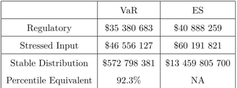
keywords: Value-at-Risk; Conditional Value-at-Risk; Economic Capital; Credit Risk; Gauss hypergeometric function; Beta-Kotz distribution..

Distribution-based risk measures with this convexity property are characterized in Section 7: As shown by Weber (2006) and Delbaen, Bellini, Bignozzi &amp; Ziegel (2014), they

When the condition (9) is met, the CAPM produces a maximum pricing error larger than that of the basic model which ignores the trade-off between risk and return. It is thus so

Although mies are well established to identify risk potential on the base of the quantity of dangerous substances (Airnexe I of the Councii Directive 96/82/EC), there is no