HAL Id: hal-01587391
https://hal.archives-ouvertes.fr/hal-01587391
Submitted on 1 Mar 2021HAL is a multi-disciplinary open access
archive for the deposit and dissemination of sci-entific research documents, whether they are pub-lished or not. The documents may come from teaching and research institutions in France or abroad, or from public or private research centers.
L’archive ouverte pluridisciplinaire HAL, est destinée au dépôt et à la diffusion de documents scientifiques de niveau recherche, publiés ou non, émanant des établissements d’enseignement et de recherche français ou étrangers, des laboratoires publics ou privés.
230Th using stratigraphical and coevality constraints
Matthieu Roy-Barman, Edwige Pons-Branchu
To cite this version:
Matthieu Roy-Barman, Edwige Pons-Branchu. Improved U–Th dating of carbonates with high initial 230Th using stratigraphical and coevality constraints. Quaternary Geochronology, Elsevier, 2016, 32, pp.29 - 39. �10.1016/j.quageo.2015.12.002�. �hal-01587391�
1
Improved U-Th dating of carbonates with high initial
230Th using
1stratigraphical and coevality contraints
2
3
4
Matthieu Roy-Barman
*and Edwige Pons-Branchu
56
7
Laboratoire des Sciences du Climat et de l’Environnement
8LSCE/IPSL, CEA-CNRS-UVSQ, Université Paris-Saclay
9F-91198 Gif-sur-Yvette, France
1011
12
Quaternary Geochronology, Volume 32, April 2016, Pages 29–39
13 14 15 16 17 18 19 20 21 *
Corresponding author ([email protected])
22 23
2 1
Abstract
2
With high precision measurements now achievable by MC-ICPMS, the uncertainty on
3
the initial 230Th content can be the major source of uncertainty for U-Th ages of carbonates.
4
The initial 230Th content is usually derived from the 232Th content of the sample and the initial
5
230
Th/232Th ratio calculated using isochron techniques or using stratigraphical constraints
6
along the speleothem growth axis. These two methods are based on different hypotheses and
7
have not been couple previously. Here, we present a new algorithm called STRUTages that
8
combines stratigraphical and coevality constraints in order to obtain the best estimate on the
9
initial 230Th/232Th ratio of each sample. STRUTages and isochron results are compared on a
10
suite of speleothems and a coral core. Comparison of the U-Th and growth-band counted ages
11
of the coral core demonstrates the validity of the STRUTages approach. An Octave
(Matlab-12
compatible) script allowing the use of stratigraphical and coevality constraints is provided.
13
14
Keywords: STRUTages; U-Th dating; speleothem; coral; isochron; stratigraphical; coeval
15 constraints 16 17 Highlights: 18
* We present a new method to constrain the initial 230Th content of coeval samples.
19
* It is compatible with the stratigraphical constraint method of Hellstrom (2006).
20
* Combination of both methods allows an improved dating of carbonates.
21
* The method is validated on independently dated (growth band counting) samples.
22
* A script performing both stratigraphical and coeval sample constraints is provided.
23 24
3
1. Introduction
1
The 230Th-234U-238U dating method is widely applied to carbonate samples
2
(speleothems, corals). It generally allows an accurate determination of the age of these
3
paleoclimatic and paleoenvironmental archives over the last 500 ka. This method assumes that
4
the carbonate has remained a closed system since its formation and that all the 230Th in the
5
sample comes from the radioactive decay of 234U. However, for speleothems and to a lesser
6
extent for corals, this last assumption is often false and this can have a significant effect on
7
the apparent age, particularly for young (< 50 ka) speleothems and/or speleothems with a low
8
U content and/or a high detrital Th content. It is therefore necessary to correct for the 230Th
9
present in the carbonate at the time of its formation. It becomes all the more critical with the
10
high analytical precision provided by MC-ICPMS, the U-Th content of most carbonate
11
sample can be determined at a permil or sub-permil level, so that the uncertainty on the initial
12
230
Th content of the speleothem becomes a significant, if not prominent, source of uncertainty
13
on the age (Dorale et al., 2004).
14
The degree of 230Th initial is generally indicated by the presence of 232Th. In early
15
studies, it was assumed that samples with (230Th/232Th) activity ratio > 20 did not require
16
corrections (Bischoff and Fitzpatrick, 1991). However, with the improvement of dating
17
technics, more recent studies propose with that the influence of this detrital fraction on age
18
determination is significant for measured (230Th/232Th) activity ratio as high as 300
19
(Hellstrom, 2006).
20
It is possible to deduce and subtract the initial 230Th content of a speleothem or a coral
21
from its 232Th content, if the initial 230Th/232Th activity ratio is known. This initial 230Th/232Th
22
activity ratio can be estimated or determined by measurements. The average crustal U/Th
23
ratio combined with the assumption that 230Th is in secular equilibrium with 238U has been
4
widely used to estimate the initial 230Th/232Th activity ratio. However, several studies have
1
demonstrated that this value does not reflect the whole range of initial Th activity ratio,
2
because clay is not the only Th source (e.g. Beck et al., 2001; Hellstrom 2006) and because
3
the U/Th ratio in detrital particles and colloids can vary strongly (Marchandise et al., 2014).
4
Drip water in caves, sea water or modern calcium carbonate are also used to determine the
5
initial Th activity ratio (230Th/232Th)A0 at the formation of the speleothem (Hu et al., 2008,
6
Wortham et al., 2013). This initial ratio can also be deduced directly from an isochron
7
constructed with several subsamples from the same laminae (or group of laminae) of the
8
speleothem having different U/Th ratios (Dorale et al., 2004). However, (230Th/232Th)A0
9
obtained on one stratigraphical level with an isochron or by the measurement of modern
10
calcite or aragonite may not be valid throughout the speleothem or coral. More recently, the
11
“stratigraphical constraint” method was developed to determine the range of (230
Th/232Th)A0
12
that keeps speleothem samples in stratigraphical order after correction for the initial 230Th
13
content (Hellstrom, 2006). These two methods require different sample set: the isochron
14
method uses several samples of the same age, whereas the stratigraphical method uses several
15
samples of different ages. The isochron method is widely used and many researchers draw
16
upon the freely-available software Isoplot (Ludwig, 2003) to calculate (230Th/232Th)A0 in an
17
isochron diagram. On the other hand, no software performing the “stratigraphical constraint”
18
method has been published so far.
19
Recently, we developed our own routine to obtain stratigraphical constraints on very
20
young (<400 a) and detritus-rich speleothems (Pons-Branchu et al., 2014). Initially, our goal
21
was to reproduce the method described in Hellstrom (2006). However, it rapidly appeared that
22
a program would be much more practical if it could combine samples of increasing ages
23
through the speleothem (the stratigraphical method) with samples from the same
24
stratigraphical level (hereafter called subsamples), whether they are “replicates” of a given
5
layer or they are purposefully analyzed to obtain an isochron (generally, n > 2). This
1
corresponds to the effective sampling of many speleothems, indeed (Ersek et al., 2009).
2
Beyond the practical aspect of treating coeval and non-coeval samples, we primarily aim at
3
better constraining the initial 230Th content of the speleothem by combining the information
4
brought by all available samples in a self-consistent manner. Indeed, it is not straightforward
5
to combine the uncertainties obtained on the same speleothem by isochron(s) and
6
stratigraphical constraints because these two methods are based on different assumptions and
7
they use common information so that they are not independent and related in a complex
8
manner.
9
We have developed a new method to evaluate the age of coeval subsamples. This
10
method is compatible in terms of assumptions and calculation process with the stratigraphical
11
method developed by Hellstrom (2006). Here, we describe this method, present a few
12
applications illustrating the possibility and limits of the method and provide an open source
13
program called STRUTages (STRatgraphical and coeval constraints on U-Th ages) that
14
allows applying the stratigraphical constraint method (with or without coeval sub-samples) to
15
a broad range of datasets.
16
17
2. Method
18
2.1. Principle of the stratigraphical constraints from non-coeval samples
19
U-Th ages, (230Th/232Th)A0 and corresponding uncertainties were calculated following
20
the stratigraphical method developed by Hellstrom (2006), which is based on a Monte Carlo
21
simulation (see description in Albarède, 1995, for example). Monte Carlo estimates of errors
22
of a function are obtained by repeatedly perturbing (N trials) the input data according to their
23
assigned errors and error distribution. At each trial, random values are generated to simulate:
6
1- measured 234U/238U, 232Th/238U and 230Th/238U activity ratios expressed as
1
(234U/238U)A, (232Th/238U)A and (230Th/238U)A (with Gaussian distributions centered on the
2
mean measured ratios and with two standard deviations (2) of the distribution given by the
3
two standard deviation on the measured ratios). There is no covariance between these ratios,
4
so -counting data cannot be treated with STRUTages.
5
2- Mean (230Th/232Th)A0 of the speleothem: Ri_mean. This is chosen from a large range
6
of plausible values (exponential distribution of the activity ratio ranging from 0.1 to 30)
7
3- Maximum percentage of variability of (230Th/232Th)A0 within the speleothem
8
(uniform distribution ranging from 0% to 100%): Ri.
9
4- For each sample analyzed in the speleothem, a specific Ri within the range defined
10
by Ri_mean and by the maximum percentage of variability Ri: uniform distribution ranging
11
from Ri_mean - Ri to Ri_mean + Ri.
12
Step 4 defines the individual (230Th/232Th)A0 ratios (Ri) of each simulated sample of the
13
speleothem within the range determined by steps 2 and 3.
14
Step 5: trials with no physical meaning (if they are just due to the statistical
15
uncertainties on the analyses) or corresponding to an open system behavior were discarded.
16
This was the case when:
17
- (230Th/238U)A < (232Th/238U)A × Ri (i.e. less 230Th in the sample today than at the time of
18
formation)
19
- (230Th/238U)A – 1> ((234U/238U)A -1) × 230 /(230 -234) (i.e. sample plotting on the right of
20
the infinite age line in a (230Th/238U)A versus (234U/238U)A -1) diagram and corresponding to
21
the “forbidden zone” for which no finite age exists).
22
7
Sample ages were calculated for each trial with the randomized values obtained at
1
steps 1 and 5, by solving numerically the equation:
2 3
1 1 1 / / / 1 1 / 234 230 230 234 230 230 238 234 0 232 230 238 232 238 230 t A A A t A e U U Th Th U Th e U Th 4 5Any trial in which the calculated ages were not in the stratigraphical order or in which
6
negative ages were obtained were discarded (Fig. 1a,b). From 104 to 1010 iterations were
7
performed to obtain at least a few hundred valid solutions with positive ages in the
8
stratigraphical order. Only these valid iterations were averaged to determine the most
9
probable ages and (230Th/232Th) A0 in the speleothem or coral (hereafter called “archive”).
10
For a given Ri_mean -Ri pair, a single successful trial is a sufficient condition to
11
guarantee that the samples can be in stratigraphical order within the analytical uncertainties
12
(Fig. 1.a). However, it is not a necessary condition because a single trial does not cover the
13
whole range of uncertainty on each sample age (Fig 1.b). Nevertheless, with the large number
14
of trails performed, it is likely that the successful trails should allow a reasonable mapping of
15
the valid Ri_mean -Ri pairs.
16
When two or more coeval subsamples from the same stratigraphic level are present in
17
the speleothem or the coral, two different constraints can be used to account for these
18
subsamples: the loose coevality constraints and the strict coevality constraints. We describe
19
these in the following sections.
20
21
22
8
2.2. Weak constraints for “loosely” coeval samples: the loose coevality constraints
1
When two or more subsamples of the same stratigraphical level of the archive are
2
analyzed, they are not compared to each other. They are just compared with the sample of the
3
previous and of the next stratigraphic level. The ages of these subsamples are simply replaced
4
by a doublet made of the lowest and the highest ages among the subsamples. This doublet
5
then replaces the whole subsamples suite in the sample series for the stratigraphical age test.
6
This treatment corresponds to a weak constraint imposed by the subsamples on Ri_mean
7
and Ri. The subsamples just have to be younger than the sample from the previous (older)
8
level and older than the next sample (younger) level. However, these subsamples do not have
9
to have the same age. It corresponds to a situation where the replicates were sampled in an
10
area where the laminae are poorly visible and/or of very slow growth rate, so that the
11
synchronicity of the “replicates” is not certain. From the modeling point of view, it provides a
12
screening of Ri_mean-Ri pairs allowing the stratigraphical order of the samples. These pairs
13
will be used in the next step to add up age constraints on coeval subsamples.
14
15
2.3. Strong constraints for strictly coeval samples: the strict coevality constrain.
16
When subsamples of one or several stratigraphical levels are present, we add new
17
constraints: the ages of all the subsamples from the same level must be equal within analytical
18
uncertainties (Fig. 1ef). We note that it is not sufficient to take the intersection of the age
19
ranges of the subsamples calculated in Section 2.3., because the initial 230Th correction
20
introduces a strong covariance between the ages of the subsamples (see Section 3.2). This
21
effect can be easily understood by considering two subsamples with partly overlapping error
22
bars after the “loose coevality constraints” test: discarding trials with the oldest ages of the
9
oldest subsamples (these ages stand above the age intersection of the subsamples) will also
1
discard the oldest ages of the youngest subsample (although they belonged to the common age
2
range) because all these ages are likely to have been obtained with same the lowest Ri_mean
3
values. Hence, two replicates having a common age range with the “loose coevality
4
constraints” may end up with significantly smaller age ranges after the “strict coevality
5
constraints”. In some case, the overlapping may disappear and the trial is then discarded.
6
In the previous sections, at each trial, the stratigraphical test was based on only one
7
randomly-chosen age of each sample because it was sufficient to set ages in order, but it is not
8
sufficient to determine if the subsample ages are equal. The age range of each sample was
9
obtained by compiling the age of the successful trials.
10
We must now determine for each successful Ri_mean-Ri pairs obtained at the Section
11
2.2. if the subsample ages are equal within uncertainties. For each successful pair, the
12
(234U/238U)A, (232Th/238U)A and (230Th/238U)A are randomized about 1000 times and used to
13
calculate the age range of each sample (subsamples or not). The age ranges of all replicates
14
from the same layer are then compared to determine their intersection. Only trials with all
15
ages in the stratigraphical order and replicate ages within the replicate age intersection are
16
selected as valid. All other trials are discarded. Hence, we obtain for each sample and
17
subsample an age range that fulfill within the analytical uncertainties both the stratigraphical
18
order for sample from different layers and the synchronicity of subsamples of a given
19 stratigraphical level. 20 21 2.4. Computing considerations 22
10
The program was computed using the Octave freeware
1
(http://www.gnu.org/software/octave/). Octave is compatible with Matlab and it can be
2
enabled on Linux, OS X, BSD and Windows operating systems. Here we use Octave 4.0.0 on
3
a PC computer with the Windows operating system. Due to the large number of trials (up to
4
1010) required to obtain enough valid solutions, constraints exist for both the running time of
5
the program and the number of trials that can be stored in the memory.
6
The calculation time was optimized by using matrix operations whenever it was
7
possible. Equation 1 was solved numerically to obtain the sample ages. We initially used the
8
built-in functions of Octave (fsolve and fzero) to solve Equation 1. However, they turned
9
out to be slow when solving a large number of equations. Therefore, we used the
Newton-10
Raphson algorithm that generally converges rapidly and that can be written under a matrix
11
form to solve thousands of equations simultaneously (Albarède, 1995, Quarteroni and Saleri,
12
2006). The effectiveness of the algorithm convergence was tested by:
13
- calculating the evolution of the (234U/238U)A and (230Th/238U)A activity ratios in a
14
closed system with prescribed values of the (234U/238U)A0 activity ratio ranging from 0.8 to 10,
15
of the prescribed (230Th/238U)A0 activity ratio equal to zero and for prescribed ages ranging
16
from 1 a to 800 ka which are, effectively, the lower and upper limits to use U-Th dating. The
17
(232Th/238U)A ratio was set to zero because the purpose was only to check the algorithm
18
convergence.
19
- recalculating the sample age with (234U/238U)A and (232Th/238U)Aas input values
20
- comparing prescribed and calculated ages.
21
The calculated age deviates from the true age by less than 0.001 ‰ for a sample of 1 a
22
and no more than 0.1 ‰ for a sample of 800 ka. This is negligible compared to the
23
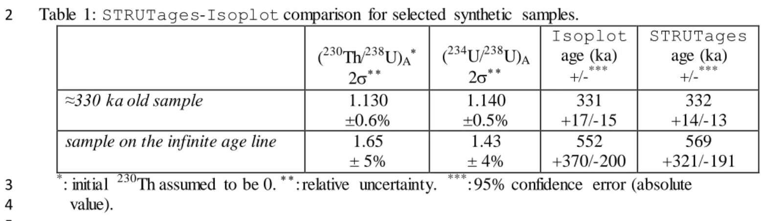
propagation of statistical uncertainties on the measurement. There is very good agreement
11
between the ages calculated on individual samples by STRUTages and Isoplot (Tab.
1
1), as illustrated by 2 numerical examples derived from Ludwig (2003).
2
The STRUTages.m (Santa Elina data) and STRUTages_acc.m (Newton algorithm
3
accuracy test) scripts and the user manual are given in electronic supplements.
4
5
2.5. Carbonate samples for program testing
6
In the following, the impact of the age correction model on carbonate dating is
7
illustrated by two speleothems in contrasting environments and one coral core:
8
- A detritus-rich and young speleothem sampled in the Santa Elina prehistoric shelter
9
(15°28’S, 56°48’W, Mato Grosso, Brasil). In this 9 cm-long stalagmite, laminated and porous
10
zones alternate. U-Th data suggests ages younger than 10 ka (Pons-Banchu and Fontugne,
11
unpublished data), whereas stratigraphically-ordered 14C ages suggest that the speleothem age
12
is less than 560 a (Fontugne, unpublished data). This is an upper limit because no dead carbon
13
correction is applied for these young ages. In this speleothem, three stratigraphical levels were
14
analyzed. For one of these level, 3 subsamples were analyzed (Table ES1 in the electronic
15
supplement).
16
- A detrital-rich and young (< 5500 a) speleothem sampled in the Rupt du Puits cave in the
17
East of France (Pons-Banchu, 2001; Jaillet et al., 2006). This speleothem developed in an
18
active karstic system covered by Cretaceous deposits (clay and sands). Eight stratigraphical
19
levels of this speleothem were analyzed (Table ES2 in the electronic supplement). For one of
20
these levels, three subsamples were analyzed.
21
- A subtidal coral core (92MC) from the Espiritu Santo island (Vanuatu) in the Eastern Pacific
22
ocean (Shen et al., 2008). The coral material expected to be less than 100 years old. It lived in
23
an open-ocean environment with no direct riverine inputs. However, the 230Th/232Th ratio of
12
the local seawater varies due to deep water upwelling during La Nina events. It has been dated
1
by both U-Th and band-counting in order to test the accuracy of young U-Th ages. Therefore,
2
it gives a unique opportunity to test the STRUTages method. Six stratigraphical levels were
3
analyzed in this core (Table ES3 in the electronic supplement). Four sub-samples were
4
analyzed for each of the two youngest levels:
5
- Subsamples (1#a to 1#d) of the youngest level with an age of 13 ± 0.5 a
6
determined by growth band counting do not plot on a single isochron (Shen et al.,
7
2008). Three subsamples (1#a to 1#c) yield an acceptable isochron age of 12 ± 1.3
8
a and an initial activity ratio Ri = 1.0. The age of the other subsample (1#d) when
9
corrected with a Ri value of 1.0 and yielded an age of 19.0 ± 1.2 a. This
10
overestimated age comes from an underestimation of the Ri value of this
11
subsample which may have grown during a short upwelling event (see below).
12
- Four subsamples (2#a to 2#d) with an age of the 30.5 ± 0.5 a determined by
13
growth band counting yield an isochron age of 29.2 ± 1.3 a and Ri = 4.5. This high
14
Ri value may be related to the upwelling of deep water Shen et al. (2008).
15
16
3. Results
17
For each archive, we first present the ages calculated with strict coevality constraints
18
only and we compare them with isochron ages obtained with Isoplot. Then, we present the
19
results obtained with the STRUTages with the loose and strict coevality constraints on the
20
whole sample set. Uncertainties on age and Ri are given as 95% probability errors (5th and 95th
21
percentiles because some age and Ri distributions are not Gaussian). Combining the mean
22
(normally associated with the standard deviation) and percentiles (normally associated with
13
the median) may appear mathematically heterodox, but it is consistent with Isoplot format
1
for non-Gaussian age distributions (Ludwig, 2003).
2
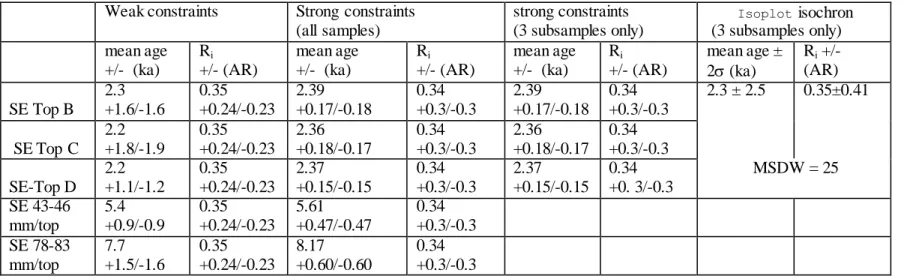
3.1. Santa Elina
3
U-Th ages (2.39 ± 0.28, 2.36 ± 0.29 and 2.37 ± 0.22 ka) of the three coeval
4
subsamples obtained with the strict coevality constraints are compatible within the uncertainty
5
of the isochron age of 2.3 ± 2.5 ka calculated with suing Isoplot.
6
The five samples can be placed in stratigraphical order for very low values of the Ri
7
(<1%) with or without coeval subsample constraints (Table 2, Figure 2a). There is a clear
8
decrease in the uncertainties of ages when coeval subsample constraints are included (Figure
9
2b). This goes together with a reduction of the range Ri values when coeval subsample
10
constraints are included. We note that the ages of the three coeval subsamples are identical
11
and have identical uncertainties whether they are calculated with or without the stratigraphical
12
constraints of the other samples. It means that in the case of Santa Elina, the age constraints
13
come only from the three coeval samples at the top of the speleothem and that putting these
14
samples in stratigraphical order with the 2 older samples brings no more constraints on age
15 and Ri. 16 17 3.2. Rupt du Puits 18
The age of the three coeval subsamples of the Rupt du Puits speleothems are not very
19
precisely constrained (≈ 5.3 ± 0.4 ka) by the coeval constraints alone because there is an
20
insufficient range of 232Th-238U for the samples (Table 3). This age is consistent within
21
uncertainties with the isochron age obtained with Isoplot (5.6 ± 0.7 ka). The ages obtained
22
with the stratigraphical constraints alone (4.92 +0.15/-0.16 ka, 4.8 +0.13/-0.12 ka, 4.94
23
+0.14/-0.15 ka) fall on the low end of the estimates made with the coeval constraints alone.
14
The stratigraphical constraints give smaller uncertainties (Fig; 3, Tab. 3) due to the occurrence
1
of much larger range of 232Th/238U fractionation along the speleothem (up to a factor 50).
2
Adding the strict constraints of coeval samples to the stratigraphical constraints provides a
3
small but significant improvement of the uncertainty of about 10% for each sample.
4
5
3.3. Santo coral core
6
It is not possible to obtain successful simulations for the four subsamples of the
7
youngest stratigraphical level or for the whole speleothem with Ri values lower than ≈ 50%.
8
(Fig. 4). Therefore, we calculate ages and Ri values for Ri < 70%. This value was chosen a
9
priori and somewhat arbitrarily.
10
The ages determined by STRUTages on the two sets of subsamples of the first and
11
second levels are consistent within uncertainties with the ages determined with Isoplot. As
12
for the Santa Elina and for the Rupt du Puits speleothems, uncertainties determined by
13
STRUTages are generally (4 point data sets of level 1 and 2) smaller than uncertainties
14
determined with Isoplot of the coral core. However, very consistent results are obtained
15
for the 3 point data set of the youngest level by STRUTages (14.2 +1.5/-1.1 y, 14.1+0.9/-0.8
16
a and 14.5 +0.8/-0.9 a) and Isoplot (14.2±1.0 a) (Tab. 4).
17
All the ages calculated by STRUTages with the coeval subsample constraints agree
18
within uncertainties with the ages determined by band counting (Figure 5).
19
20
4. Discussion
21
4.1 Comparing STRUTages with isochron ages for coeval subsamples
15
Isochrones are the most appropriate method to determine the age of coeval samples
1
(e.g. Allègre, 2008). Therefore, it is important to compare STRUTages ages with isochron
2
ages. Since 230Th and 234U are both radioactive and radiogenic, isochron age determination is
3
often done by drawing isochrons in the (230Th/238U)A versus (232Th/238U)A and (234U/238U)A
4
versus (232Th/238U)A diagrams or other diagram pairs that completely define the 234U -238
U-5
230
Th -232Th system (Geyh, 2008). However, full uncertainty propagation is difficult with
6
paired diagrams because they share common information. This difficulty is circumvented by
7
considering a single isochron line in three-dimensional space, i.e (230Th/238U)A -(234U/238U)A
-8
(232Th/238U)A, which can be done using the Isoplot program (Ludwig and Titterington,
9
1994, Ludwig, 2003).
10
The three fundamental assumptions of an isochron are that (1) the samples must have
11
been formed at the same time, (2) their parent and daughter isotope ratios were initially
12
homogeneous which corresponds to a single source of initial Ri and (3) they have behaved as
13
a closed-system. When sample scattering around the isochron exceeds analytical errors, at
14
least one of the following failures affects the samples: 1) multiple detrital components (Dorale
15
et al. 2004), 2) multiple ages, or 3) an open-system history (Borsato et al., 2003).
16
In contrast to the single Ri value (corresponding to a single detrital source) assumption
17
of the isochron method, the basis of the age calculation with the strict coevality constraints is
18
to adjust the Ri ratio of each subsample in order to obtain a common age for all these
19
subsamples. With different assumptions, STRUTages and isochron methods may produce
20
different ages. In Section 3, we noted that there is a good agreement (within uncertainties)
21
between the mean U-Th ages calculated with the different methods, but that isochron
22
uncertainties are often larger than the STRUTages uncertainties. It can be related to the data
23
scattering around the calculated isochron, which is quantified by the Mean Square of
24
Weighted Deviates, or MSWD (Ludwig, 2006). MSWD values >> 1 indicate more scatter
16
than predicted by the analytical errors. Values ≤ 1 correspond to a good fit of the data by the
1
isochron. Looking at the examples given in Section 3, it appears that:
2
-when MSWD < 1 (e.g. subsamples 1#1-3 of the Santo coral core and Rupt du Puits
3
speleothem), both methods give similar uncertainties. In this case, the different subsamples
4
plot on the isochrons with a well-defined Ri value. The age uncertainty corresponds to the
5
analytical scattering and there is no additional uncertainty such as Ri variability due to
6
multiple detrital components. In this favorable case, STRUTages and Isoplot should give
7
similar results, as it is the case for the subsamples 1#a,b,c of the Santo coral . In the Rupt du
8
Puits case, the ages given by STRUTages (≈ 5.3 ± 0.4 ka) and Isoplot largely overlap
9
(5.6 ± 0.7 ka) but the mean age of STRUTages is about 0.3 ka older than the mean
10
Isoplot age. This is because Ri (= 0.2 ± 0.6) is poorly defined by Isoplot (there is small
11
range in 232Th/238U between the three coeval sub-samples, see Table ES2) and it includes
12
negative values with no physical reality (but that may correspond to an open-system
13
behavior). Conversely, STRUTages simulates only positive Ri values (Ri = 0.36
+0.37/-14
0.24). As a consequence, STRUTages calculates larger initial 230Th corrections and lower
15
mean ages than Isoplot.
16
- when MSWD >> 1 (Santa Elina, subsamples 1#1-4 of the Santo coral core), the
17
samples are scattered around the isochron: the fit is poor. Isoplot propagates this scattering
18
into to the age uncertainty, whereas STRUTages minimizes this scattering by adjusting the
19
Ri of each sample to obtain a common age for the whole subsample set. Hence, for large
20
MSWD values, the different hypothesis of Isoplot and STRUTages lead to different
21
uncertainties. Therefore checking the validity of these hypotheses will be crucial for
22
STRUTages (see Section 4.2.).
23
17
4.2 Combining stratigraphical and strict coevality constraints
1
The stratigraphical constraints method is presented as possibly more appropriate to
2
correct of speleothem samples for detrital contamination than isochron because it explicitly
3
assumes that the detrital Th is of variable isotopic composition, whereas isochron techniques
4
assumes a homogeneous detrital end-member that may not be representative of the whole
5
speleothem (Hellstrom, 2006). Why then do we introduce strict coevality constraints with
6
STRUTages? While STRUTages calculates Ri ranges that bring coeval sub-samples within
7
the same age range, it does not directly use these Ri values to correct for the initial thorium of
8
the samples collected on other stratigraphical level like one would do with an isochron.
9
Instead, STRUTages selects for each sample the range of Ri that is most likely to fulfill both
10
coevality and stratigraphic constraints. It influences the non-coeval sample ages because:
11
- The restricted age range of coeval samples puts an upper limit on the possible ages
12
of younger samples and a lower limit on the possible ages of older samples)
13
- the Ri range imposed by strict coevality constraints may restrict the range of
14
possible Ri of the whole sample set or require high Ri to fulfill all the constraints
15
simultaneously.
16
When the Ri ranges of all the samples have a common intersection (this is the case for
17
Santa Elina and Rupt du Puits), any Ri value in this intersection can be used to correct the
18
initial Th content of all the samples and will leave them in the stratigraphical order.
19
Conversely, when the intersection of all the Ri ranges is null, a certain range of variability
20
(Ri) is required leave all the samples in the stratigraphical order (Santo coral core with
21
strong constraints). These two types of behavior were extensively discussed for the
22
stratigraphical method without coevality constraints (Hellstrom, 2006, Pons-Branchu et al.,
23
2014).
18 1
The Santa Elina and the Rupt du Puits speleothems are two extreme cases of the
2
relative weight of stratigraphical and strict coeval samples:
3
- For Santa Elina, most of the constraint on Ri come from the strict coevality
4
constraints on the 3 coeval subsamples. This is reflected by the significant
5
decrease of the uncertainties on ages and Ri when the strict coevality constraints
6
are included (Figure 2) and to the similar age and Ri ranges obtained for the three
7
SE-top samples alone or with SE 43-46 and SE 78-83 (Table 2, with strict
8
coevality constraints).
9
- By contrast, in the Rupt du Puits speleothem, most constraints come from the
10
stratigraphical constraints on the non-coeval samples due to the large range in
11
232
Th/238U (up to a factor 50) ratio along the speleothem (see electronic
12
supplement, Table ES2). This is reflected in the similar uncertainties on ages and
13
Ri with or without strict coevality constraints (Fig. 3b). As a consequence, the ages
14
of the 3 subsamples (R69-6abc) are much better defined by the weak constraints
15
applied to the whole speleothem than by the strict constraints on coeval samples
16
alone (Tab. 3). The impact of the strong constraints on coeval samples is restricted
17
to a 10% decrease of the uncertainties, when the strong constraints on coeval
18
samples are applied to the whole speleothem.
19
The two previous examples illustrate the interplay between the different constraints
20
used in the model. However, they do not guarantee the validity of the modeled ages.
21
For the Santa Elina speleothem, there is a significant disagreement between the ages
22
obtained with the loose and strict coevality constrains and the 14C ages that are all less than
23
550 a. This may be due to:
19
1- U-Th ages can be overestimated compared to 14C ages in case of U loss (Plagnes
1
et al. 2003). This is possible considering that the Santa Elina speleothem grows in
2
a rock shelter. Alternatively, 14C-rich young organic matter can contaminate
3
carbonates but it usually concerns old carbonates (Holmgren et al., 1994; Goslar et
4
al., 2000).
5
2- The (230Th/232Th)A ratios of the Santa Elina samples range from 0.6 to 1.9, within
6
the range of possible values for the (230Th/232Th)A0 ratio. So, it is possible that the
7
Santa Elina speleothem is very young (550 a or less) so that (230Th/232Th)A0 ≈
8
(230Th/232Th)A and that (230Th/232Th)A variations just reflect (230Th/232Th)A0
9
variations. In this case, there is no discrepancy between the U-Th and the 14C ages
10
(remember that the 14C ages are not corrected for the dead carbon).
11
It is beyond the scope of this article to choose between these two hypotheses.
12
However it highlights two important methodological implications:
13
1) If the U-Th behaves as an open system, STRUTages ages are meaningless.
14
2) Whatever the real ages are, a trivial solution is that all Santa Elina U-Th ages are
15
equal to zero if (230Th/232Th)A0 ≈ (230Th/232Th)A. However STRUTages does not
16
find this solution. One reason is that the exponential distribution used to
17
randomized Ri_mean favor low R i_mean values (and thus large ages). Thus trials with
18
Ri ≈ 0.35 are more likely to be appear than trials with Ri ≈ 1.6-1.9 necessary to set
19
the ages of samples SE 43-46 mm/top and SE 78-83 mm/top close to zero.
20
Even if the zero age solution is statistically less probable than the one proposed by
21
STRUTages, it does not mean that it is the correct one. In such a case with
22
(230Th/232Th)A ratios in the range permitted for (230Th232Th)A0 and with high
20
(232Th/238U)A, ratios geochemical arguments or absolute dating are required to
1
determine the correct age.
2
3
The Santo coral core provides the opportunity to compare modeled age with true ages
4
obtained by growth band counting on a coral in which variations of the initial (230Th/232Th)A
5
activity ratio are clearly documented. The good agreement (within uncertainties) between the
6
modelled and the counted ages gives confidence (at least in this example) to the reliability of
7
the STRUTages method. The uncertainties on the ages modeled with STRUTages are
8
generally larger than those obtained with isochrons by Shen et al. (2008). However, two
9
points must be noted:
10
- the good agreement between the U-Th ages of Shen et al. (2008) and counted ages
11
for samples 3,4,5 and 6 is due to the choice of a Ri of 1 (isochron 1) rather than 4.5
12
(isochron 2) for these samples. This choice was obviously influenced by the
13
known counted ages. However, generally carbonates are dated by the U-Th method
14
because no counted age is available.
15
- To be self-consistent in their approach, Shen and coworkers apply a Ri ratio of 1.0
16
to sample 1#d and hence significantly overestimate its age.
17
Hence, STRUTages combines efficiently the stratigraphical constraints of Hellstrom
18
(2006) and the constraints on coeval samples that are traditionally treated by isochrons.
19
One of the sources of uncertainty with the stratigraphical constraint model is the
20
maximum value of Ri (the variability of the Ri ratio within the speleothem) that should be
21
used to evaluate the ages and their uncertainties. In some cases, the variability of Ri is well
22
established in corals (Shen et al, 2008) or in speleothems (Dorale et al., 2004). However, there
21
is a risk that a need of using large values of Ri to set samples in stratigraphical order
1
corresponds to an open system problem (Hellstrom, 2006). While the stratigraphic model does
2
not favor a particular Ri value, the few studies using the stratigraphical constraint methods
3
have used Ri values on the low side of the possible range (Hellstrom, 2006, Pons-Branchu et
4
al., 2014). It has the advantage of reducing the uncertainties on the modelled ages but may
5
lead to an underestimation of these uncertainties. The problem is that at present only too few
6
studies focus on the variability of the (230Th/232Th)A activity ratio of detrital material in
7
speleothems (Beck et al., 2001, Carolin et al. 2013, Labonne et al., 2002, Meyer et al., 2012,
8
Richards and Dorale, 2003, Yuan et al., 2004, Moseley et al., 2014) or corals (Shen et al.,
9
2008). Seawater is used to determine the (230Th/232Th)A0 activity ratio of corals (Shen et al.,
10
2008). However, the residence time of Th is very short (1 year at most) in the surface ocean
11
so that the (230Th/232Th)A activity ratio of seawater may significantly evolve through time.
12
More studies are needed to have a better view of the variability of Ri in speleothems and
13
corals.
14
STRUTages adjusts the Ri of each coeval subsample of a given stratigraphical level
15
to obtain the same age for each subsample. Unlike the isochron method, it does not consider
16
the possibility for open system behavior. In general, speleothems develop in protected
17
environments, so that open system behaviors are rare. When it occurs, it can be detected by
18
mineralogical studies (Borsato et al., 2003, Scholz et al., 2014). In corals, the detection of
19
calcite in aragonitic coral species is a strong indication of open system behavior. The
20
234
U/238U initial ratio in corals is also used as a clue for open or closed system behavior, as
21
this ratio is expected to display small variations over the past climatic cycles (Robinson et al.,
22
2006). However, some diagenetic alterations could be not detected by these means and further
23
geochemical analyses could be necessary (Bar-Matthews et al., 1993; Pons-Branchu et al.,
24
2005). If, for a given speleothem, the range of the (230Th/232Th) activity ratio of the potential
22
detrital thorium sources is known, STRUTages is well suited to propagate the corresponding
1 uncertainties. 2 3 Conclusion 4
The combination of the stratigraphical constraints proposed by Hellstrom (2006)
5
together with the strict coevality constraints proposed here provides a robust way to
6
constraints the initial (230Th/232Th) activity ratio of stratified carbonates. Compared to the
7
isochron method it has the advantage of not requiring the assumption of a single
8
(230Th/232Th)A0 initial activity ratio value and to allow the change of this ratio along the
9
speleothem/coral or within a stratigraphical horizon. From that respect, the strict coevality
10
constraints provide an alternative to isochrons to calculate the age of samples with less
11
restrictive assumption. The field of application of this method is not restricted to carbonate
12
dating. It could be useful for U-Th dating of Quaternary-aged lava flow sequences and may be
13
also applicable to other isotopic systems with initial isotope heterogeneities.
14
15
Acknowledgements:
16
Many thanks to Michel Fontugne for his kind permission to use the Santa Elina data.
17
We are grateful to Ken Ludwig for his prompt answers to our questions on Isoplot. We
18
thank David Richards and an anonymous reviewer for their constructive comments. This
19
project was supported by the “Paris 2030” and Ec2CO programs by grants to E P-B. This is
20
LSCE contribution number 5582.
21
23 1
References
2
Albarède, F., 1995. Introduction to Geochemical Modeling. Cambridge University Press,
3
Cambridge.
4
Allègre, C. J., 2008. Isotope geology. Cambridge University Press, Cambridge.
5
Bar-Matthews M., Wasserburg G.J., Chen J.H.,1993. Diagenesis of fossil coral skeletons:
6
Correlation between trace elements, textures, and 234U/238U. Geochimica et Cosmochimica
7
Acta, 57, 257–276.
8
Beck, J.W., Richards, D.A., Edwards, R.L., Silverman, B.W., Smart, P.L., Donahue, D.J.,
9
Hererra-Osterheld, S., Burr, G.S., Calsoyas, L., Jull, A.J.T., Biddulph, D., 2001. Extremely
10
large variations of atmospheric C-14 concentration during the last glacial period. Science
11
292, 2453–2458.
12
Bischoff J. L. and Fitzpatrick J. A., U-series dating of impure carbonates: an isochron
13
technique using total-sample dissolution. Geochim. Cosmochim. Acta 55, 1991, 543-554.
14
Borsato, A., Quinif, Y., Bini, A., & Dublyansky, Y., 2003. Open-system alpine speleothems:
15
implications for U-series dating and paleoclimate reconstructions. Studi Trent. Sci. Nat.,
16
Acta Geol. 80, 71-83.
17
Carolin, S. A., Cobb, K. M., Adkins, J. F., Clark, B., Conroy, J. L., Lejau, S., ... & Tuen, A.
18
A., 2013. Varied response of western Pacific hydrology to climate forcings over the last
19
glacial period. Science 340, 1564-1566.
24
Dorale, J.A., Edwards, R. L., Alexander Jr, E.C., Shen, C.C., Richards, D. A., & Cheng, H.,
1
2004. Uranium-series dating of speleothems: current techniques, limits & applications. In
2
Studies of Cave Sediments (pp. 177-197). Springer US.
3
Ersek, V, Hostetler, S.W., Cheng, H., Clark, P.U., Anslow, F.S., Mix, A.C., Edwards, R.L.,
4
2009. Environmental influences on speleothem growth in southwestern Oregon during the
5
last 380 000 years. Earth Planet. Sci. Lett., 279 (3-4), 316-325.
6
Geyh, M., 2008. Selection of suitable data sets improves 230Th/U dates of dirty material.
7
Geochronometria, 30, 69-77.
8
Goslar T, Hercman H, Pazdur A, 2000. Comparison of U-series and radiocarbon dates of
9
speleothems. Radiocarbon 42, 403–414.
10
Hellstrom, J., 2006. U-Th dating of speleothems with high initial 230Th using stratigraphical
11
constraints. Quat. Geochronol. 1, 289-295.
12
Holmgren K, Lauritzen SE, Possnert G. 1994. 230Th/234U dating of a Late Pleisto cene
13
stalagmite in Lobatse II Cave, Botswana. Quaternary Science Reviews 13,: 111 – 9
14
Hu, C.-Y., Henderson, G.M., Huang, J.-H., Xie, S.-C., Sun, Y., Johnson, K.R., 2008.
15
Quantification of Holocene Asian monsoon rainfall from spatially separated cave records.
16
Earth and Planetary Science Letters 266, 221–232.
17
Jaillet, S., Pons-Branchu, E., Maire, R., Hamelin, B. & Brulhet, J., 2006. Record of Holocene
18
palaeo-groundwater floods in two stalagmites of the Rupt-Du-Puits Sytem (Barrois,
19
France). Morphological analysis of laminae and U/Th TIMS datings. Geologica Belgica, 9,
20
297-307.
25
Labonne, M., Hillaire-Marcel, C., Ghaleb, B., & Goy, J.L., 2002. Multi- isotopic age
1
assessment of dirty speleothem calcite: an example from Altamira Cave, Spain. Quaternary
2
science reviews, 21, 1099-1110.
3
Ludwig, K.R., 2003. Mathematical–statistical treatment of data and errors for Th-230/U
4
geochronology. Reviews in Mineralogy & Geochemistry 52, 631–656.
5
Ludwig K.R., Titterington, D.M., 1994. Calculation of 230Th/U Isochrons, ages, and errors:
6
Geochim Cosmochim Acta 58, 5031-5042.
7
Marchandise, S., Robin, E., Ayrault, S., and Roy-Barman, M., 2014. U–Th–REE–Hf bearing
8
phases in Mediterranean Sea sediments: Implications for isotope systematics in the ocean.
9
Geochimica et Cosmochimica Acta, 131, 47-61.
10
Meyer, M. C., Spötl, C., Mangini, A., & Tessadri, R., 2012. Speleothem deposition at the
11
glaciation threshold—An attempt to constraint the age and paleoenvironmental
12
significance of a detrital-rich flowstone sequence from Entrische Kirche Cave (Austria).
13
Palaeogeography, Palaeoclimatology, Palaeoecology, 319, 93-106.
14
Moseley G.E., Spötl C., Svensson A., Cheng H., Brandstätter S. and Edwards, L., 2014.
15
Multi-speleothem record reveals tightly coupled climate between central Europe and
16
Greenland during Marine Isotope Stage 3. Geology 42;1043-1046
17
Plagnes, V., Causse, C., Fontugne, M., Valladas, H., Chazine, J. M. and Fage, L. H., 2003.
18
Cross dating (Th/U-14 C) of calcite covering prehistoric paintings in Borneo. Quaternary
19
Research, 60, 172-179.
20
Pons-Branchu, E., 2001. Datation haute résolution de spéléothèmes (230Th/234U et 226Ra/238U).
21
Application aux reconstitutions environnementales autour des sites du Gard et de Meuse /
22
Haute-Marne. Thesis. Univ. Aix-Marseille, 190 p.
26
Pons-Branchu, E., Douville, E., Roy-Barman, M., Dumont, E., Branchu, P., Thil, F., Frank,
1
N., Bordier, L. and Borst, W., 2014. A geochemical perspective on Parisian urban history
2
based on U-Th dating, laminae counting and yttrium and REE concentrations of recent
3
carbonates in underground aqueducts. Quaternary Geochronology 24, 44-53.
4
Pons-Branchu, E., Hillaire-Marcel, C., Deschamps, P., Ghaleb, B. and Sinclair, D. J., 2005.
5
Early diagenesis impact on precise U-series dating of deep-sea corals: Example of a 100–
6
200-years old Lophelia pertusa sample from the northeast Atlantic. Geochimica et
7
Cosmochimica Acta, 69, 4865-4879.
8
Quarteroni, A. and Saleri, F., 2006. Scientific Computing with MATLAB and Octave, vol. 2
9
of Texts in Computational Science and Engineering. Springer-Verlag, Berlin Heidelberg.
10
Richards, D. A., & Dorale, J. A., 2003. Uranium-series chronology and environmental
11
applications of speleothems. Reviews in Mineralogy and Geochemistry 52, 407-460.
12
Robinson, L.F., Adkins, J.F., Fernandez, D.P., Burnett, D.S., Wang, S.L., Gagnon, A.C. and
13
Krakauer, N., 2006. Primary U distribution in scleractinian corals and its implications for
14
U series dating. Geochemistry, Geophysics, Geosystems 7, 1-20,
15
doi:10.1029/2005GC001138. Q05022.
16
Scholz, D., Tolzmann, J., Hoffmann, D. L., Jochum, K. P., Spötl, C., & Riechelmann, D. F.
17
2014. Diagenesis of speleothems and its effect on the accuracy of 230Th/U-ages. Chemical
18
Geology, 387, 74-86.
19
Shen, C. C., Li, K. S., Sieh, K., Natawidjaja, D., Cheng, H., Wang, X., and Kilbourne, K. H.,
20
2008. Variation of initial 230Th/232Th and limits of high precision U–Th dating of
shallow-21
water corals. Geochimica et Cosmochimica Acta, 72(17), 4201-4223.
27
Wortham, B.E., Banner, J.L., James, E. and Loewy, S.L., 2013. Direct Measurement of Initial
1
230
Th/232Th Ratios in Central Texas Speleothems for More Accurate Age Determination.
2
American Geophysical Union, Fall Meeting 2013, abstract #V13A-2595
3
Yuan, D.X., Cheng, H., Edwards, R.L., Dykoski, C.A., Kelly, M.J., Zhang, M.L., Qing, J.M.,
4
Lin, Y.S., Wang, Y.J., Wu, J.Y., Dorale, J.A., An, Z.S., Cai, Y.J., 2004. Timing, duration,
5
and transitions of the Last Interglacial Asian Monsoon. Science 304, 575–578.
6 7 8 9 10 11 12 13
28 1
Table 1: STRUTages-Isoplot comparison for selected synthetic samples.
2 (230Th/238U)A 2 (234U/238U)A 2 Isoplot age (ka) +/-*** STRUTages age (ka) +/-*** ≈330 ka old sample 1.130 ±0.6% 1.140 ±0.5% 331 +17/-15 332 +14/-13
sample on the infinite age line 1.65
± 5% 1.43 ± 4% 552 +370/-200 569 +321/-191
*: initial 230Th assumed to be 0. : relative uncertainty. ***: 95% confidence error (absolute
3
value).
4 5
29 1
30
Table 2: Simulation results for the Santa Elina speleothem.
Weak constraints Strong constraints (all samples) strong constraints (3 subsamples only) Isoplot isochron (3 subsamples only) mean age +/- (ka) Ri +/- (AR) mean age +/- (ka) Ri +/- (AR) mean age +/- (ka) Ri +/- (AR) mean age ± 2 (ka) Ri +/- (AR) SE Top B 2.3 +1.6/-1.6 0.35 +0.24/-0.23 2.39 +0.17/-0.18 0.34 +0.3/-0.3 2.39 +0.17/-0.18 0.34 +0.3/-0.3 2.3 ± 2.5 0.35±0.41 SE Top C 2.2 +1.8/-1.9 0.35 +0.24/-0.23 2.36 +0.18/-0.17 0.34 +0.3/-0.3 2.36 +0.18/-0.17 0.34 +0.3/-0.3 SE-Top D 2.2 +1.1/-1.2 0.35 +0.24/-0.23 2.37 +0.15/-0.15 0.34 +0.3/-0.3 2.37 +0.15/-0.15 0.34 +0. 3/-0.3 MSDW = 25 SE 43-46 mm/top 5.4 +0.9/-0.9 0.35 +0.24/-0.23 5.61 +0.47/-0.47 0.34 +0.3/-0.3 SE 78-83 mm/top 7.7 +1.5/-1.6 0.35 +0.24/-0.23 8.17 +0.60/-0.60 0.34 +0.3/-0.3
31
Table 3: Simulation results for the Rupt du Puits speleothem.
Weak constraints Strong constraints (all samples) strong constraints (3 subsamples only) Isoplot isochron (3subsamples only) mean age +/- (ka) Ri +/- (AR) mean age +/- (ka) Ri +/- (AR) mean age +/- (ka) Ri +/- (AR) mean age ± 2 (ka) Ri +/- (AR) R69-1 4.12 +0.31/-0.55 0.77 +0.12/-0.11 4.16 +0.27/-0.46 0.76 +0.09/-0.08 R69-3 4.45 +0.05/-0.04 0.77 +0.12/-0.11 4.45 +0.04/-0.04 0.76 +0.09/-0.08 R69-4 4.74 +0.10/-0.10 0.77 +0.12/-0.11 4.75 +0.09/-0.09 0.76 +0.09/-0.08 R69-6a 4.92 +0.15/-0.16 0.77 +0.12/-0.11 4.92 +0.12/-0.13 0.76 +0.09/-0.08 5.3 +0.3/-0.4 0.36 +0.37/-0.24 5.6 ± 0.7 0.2 ± 0.6 R69-6b 4.81 +0.13/-0.12 0.77 +0.12/-0.11 4.82 +0.12/-0.11 0.76 +0.09/-0.08 5.2 +0.3/-0.4 0.36 +0.37/-0.24 R69-6c 4.94 +0.14/-0.15 0.77 +0.12/-0.11 4.93 +0.12/-0.13 0.76 +0.09/-0.08 5.3 +0.3/-0.4 0.36 +0.37/-0.24 MSWD = 0.05 R69-7 5.09 +0.10/-0.10 +0.12/-0.11 0.77 +0.10/-0.10 5.09 +0.09/-0.08 0.76 R69-9 5.37 +0.07/-0.08 0.77 +0.12/-0.11 5.38 +0.07/-0.07 0.76 +0.09/-0.08
32
Table 4: Simulation results for the Santo coral core.
Weak constraints (all samples) Strong constraints (all samples) strong constraints (4 subsamples only) Isoplot isochron (4 subsamples only) strong constraints (3subsamples only) Isoplot isochron (3 subsamples only) mean age +/- (a) Ri +/- (AR) mean age +/- (a) Ri +/- (AR) mean age +/- (a) Ri +/- (AR) mean age ± 2 (a) Ri +/- (AR) mean age +/- (a) Ri +/- (AR) mean age ± 2 (a) Ri +/- (AR) 1 #1 7.6 +5.6/-6.4 2.5 +1.4/-1.2 12.0 +2.6/-3.2 1.5 +0.7/-0.6 10.4 +3.1/-3.9 1.8 +1.2/-0.9 14.2 +1.5/- 1.1 1.0 +0.3/-0.7 1 #2 12.2 +1.8/-2.2 2.6 +1.7/-1.3 12.0 +2.1/-2.8 +2.4/-1.6 2.8 10.5 +3.0/- 3.9 3.8 +4.5/-3.1 15.9±5.6 0.8±2.1 14.1 + 0.9/- 0.8 1.0 +0.2/-0.3 14.2±1.0 1.0±0.4 1 #3 12.0 +2.3/-2.9 2.6 +1.7/-1.3 12.2 +2.4/-3.2 2.5 +2.0/-1.4 10.4 +3.1/-4.0 3.4 +3.5/-2.5 14.5 +0.8/-0.9 1.0 +0.3/-0.3 MSWD = 0.37 1 #4 15.9 +2.7/-3.5 2.6 +1.7/-1.3 13.1 +2.2/-3.2 4.0 +1.6/-1.2 10.6 +3.1/-4.1 5.1 +3.0/-2.0 MSWD = 18 2 #1 31.7 +1.6/-1.9 2.6 +1.7/-1.3 31.3 +2.0/-2.3 3.1 +2.1/-1.8 29.4 +0.9/-1.0 4.6 +0.5/-0.4 2 #2 31.3 +2.1/-2.7 2.6 +1.7/-1.3 30.9 +2.6/-2.9 2.9 +2.0/-1.7 28.9 +1.0/-1.0 4.6 +0.5/-0.4 28.7±2.8 4.7±1.6 2 #3 31.0 +1.9/-2.3 2.6 +1.7/-1.3 30.6 +2.3/-2.7 +2.1/-1.7 2.9 28.9 +1.0/-1.0 4. +0.5/-0.4 2 #4 34.1 +3.5/-4.6 2.8 +1.7/-1.3 31.4 +2.6/-3.4 3.8 +1.2/-1.0 29.2 +1.1/-1.2 4.6 +0.5/-0.4 MSWD = 2.7 3 36.0 +3.1/-3.8 2.3 +1.5/-1.2 35.8 +3.2/-3.4 2.4 +1.4/-1.2 4 45.8 +0.9/-1.0 2.6 +1.7/-1.3 45.7 +1.0/-1.1 3.0 +2.1/-1.8 5 56.0 +1.7/-2.2 2.6 +1.7/-1.3 55.5 +2.3/-2.6 3.1 +2.2/-1.8 6 65.4 +5.8/-7.3 2.6 +1.6/-1.3 64. 2+7.3/-7.7 2.8 +1.7/-1.6
33
Figure Caption
1
2
Figure 1: Principle of the stratigraphical and coevality constraints as calculated in
3
STRUTages. a: example of valid simulation for a stalagmite without coeval samples. b:
4
example of discarded simulation for a stalagmite without coeval samples. Cases a and b
5
correspond to the Hellstrom (2006) approach with no coeval samples. c: example of valid
6
simulation with the loose coevality constraints applied to coeval samples. d: example of
7
discarded simulation with the loose coevality constraints applied to coeval samples. e:
8
example of valid simulation with the strict coevality constraints applied to coeval samples. f:
9
example of discarded simulation with the strict coevality constraints applied to coeval
10
samples. Circles and ellipses represent the ages simulated during one trial with the loose
11
coevality constraints. On sub-figures e and f, the small black squares represent the results of
12
the calculated ages used to reconstruct the full error-bar of the sample ages.
13
14
Figure 2: Monte Carlo simulation results for the Santa Elina speleothem. a: Ri versus Ri_mean
15
for the successful trails with the loose coevality constraints. b: Age distribution with the loose
16
coevality constraints applied to trials with Ri <1%. c: Ri versus Ri_mean for the successful
17
trails with the strict coevality constraints. d: Age distribution with the strict coevality
18
constraints applied to trials with Ri <1% (about 1000 successful trails were obtained by
19
specifically running STRUTages with Ri values <1%). Coeval samples are underlined.
20
Figure 3: Monte Carlo simulation results for the Rupt du Puits speleothem. a: Ri versus
21
Ri_mean for the successful trails with the loose coevality constraints. b: Age distribution with
22
the loose coevality constraints applied to trials with Ri <1%. c: Ri versus Ri_mean for the
34
successful trails with the strict coevality constraints. d: Age distribution with the strict
1
coevality constraints applied to trials with Ri <1% (about 1000 successful trails were
2
obtained by specifically running STRUTages with Ri values <1%). Coeval samples are
3
underlined.
4
Figure 4: Monte Carlo simulation results for the Santo coral core. a: Ri versus Ri_mean for
5
the successful trails with the loose coevality constraints. b: Age distribution with the loose
6
coevality constraints applied to trials with Ri <1%. c: Ri versus Ri_mean for the successful
7
trails with the strict coevality constraints. There is no successful trial forRi <50%. d: Age
8
distribution with the strict coevality constraints applied to trials with Ri <70%. Coeval
9
samples are underlined.
10
11
Figure 5: Comparison of the calculated ages with the counted ages of the Santo coral. a:
12
STRUTages versus counted ages. b: isochron and isochron-derived ages from Shen et al.
13
(2008) versus counted ages. The continuous line is the 1:1 line.
14
35 (1) and (2) are not in stratigraphical order Young Old Age 1 2 3 4 1 2 3 4 3 4 1 2
valid simulation discarded simulation
Young Old Age 2 1 3 4 1 2 3 4 3 4 2 1
Stratigraphical order test
(a) (b)
Young Old Age 2a 1 2b 3 1 2a 2b 3 3 2min 1 not in apparent stratigraphical order Young Old Age 1 2a 2b 3 1 2a 2b 3 3 1validsimulation discarded simulation Coeval subsamples : loose coevality constraints
(c) (d)
2c 2c 2c 2c 2max 2max 2min Young Old Age 1 2a 2b 3 1 2a 2b 3 2b 3 1 2avalidsimulation discarded simulation Coeval subsamples : strict coevality constraints
2 Young Old Age 1 2a 2b 3 1 2a 2b 3 2b 3 1 2a no overlapping
(e) (f)
2b 2b 2b 2a 2b 2a 2a 3 3 3 1 1 1 Figure 136
Sample order number
1 2 3 4 5 12 10 8 6 4 2 0 1 2 3 4 5 12 10 8 6 4 2 0 M odelled age (k a)
loose coevality constraints
0.1 1 10 0.1 1 10 100 10 1 100 10 1
strict coevality constraints
d) b) c) a) M odelled age (k a)
Sample order number
Ri (%) Ri (%) Ri Ri
37
Sample order number
5.5 5.0 4.5 4.0 3.5 5.5 5.0 4.5 4.0 3.5
Sample order number
2 4 6 8
2 4 6 8
loose coevality constrains
0.1 1 10 0.1 1 10 100 10 1 100 10 1
strict coevality constrains
d) b) c) a) M ode lled age (k a) Ri (%) Ri (%) Ri Ri M ode lled age (k a)
38
Sample order number
2 4 6 8 10 12 80 60 40 20 0 80 60 40 20 0 2 4 6 8 10 12
Sample order number loose coevality constrains
0.1 1 10 100 10 d) b) c) a) 100 10 1 0.1 1 10
strict coevality constrains
1 M odelled age (k a) Ri (%) Ri (%) Ri Ri M odelled age (k a)
39