HAL Id: hal-01066235
https://hal.inria.fr/hal-01066235
Submitted on 19 Sep 2014
HAL is a multi-disciplinary open access
archive for the deposit and dissemination of
sci-entific research documents, whether they are
pub-lished or not. The documents may come from
teaching and research institutions in France or
abroad, or from public or private research centers.
L’archive ouverte pluridisciplinaire HAL, est
destinée au dépôt et à la diffusion de documents
scientifiques de niveau recherche, publiés ou non,
émanant des établissements d’enseignement et de
recherche français ou étrangers, des laboratoires
publics ou privés.
Large Scale Sparse Optimization for Object Detection in
High Resolution Images
Aurélie Boisbunon, Rémi Flamary, Alain Rakotomamonjy, Alain Giros,
Josiane Zerubia
To cite this version:
Aurélie Boisbunon, Rémi Flamary, Alain Rakotomamonjy, Alain Giros, Josiane Zerubia. Large Scale
Sparse Optimization for Object Detection in High Resolution Images. MLSP - 24th IEEE Workshop
on Machine Learning for Signal Processing, Sep 2014, Reims, France. �hal-01066235�
LARGE SCALE SPARSE OPTIMIZATION FOR OBJECT DETECTION IN HIGH
RESOLUTION IMAGES
Aur´elie Boisbunon
✶❀✷❀✄, R´emi Flamary
✸❀②, Alain Rakotomamonjy
✹❀③, Alain Giros
✶, Josiane Zerubia
✷✶
CNES
✷INRIA
✸UNS-CNRS-OCA
✹Normandie Universit´e
DCT/SI/AP
AYIN team
Lab. Lagrange
Lab. LITIS
Toulouse, France
Sophia Antipolis, France
Nice, France
Rouen, France
ABSTRACT
In this work, we address the problem of detecting objects in images by expressing the image as convolutions between acti-vation matrices and dictionary atoms. The actiacti-vation matrices are estimated through sparse optimization and correspond to the position of the objects. In particular, we propose an effi-cient algorithm based on an active set strategy that is easily scalable and can be computed in parallel. We apply it to a toy image and a satellite image where the aim is to detect all the boats in a harbor. These results show the benefit of using nonconvex penalties, such as the log-sum penalty, over the convex❵✶penalty.
Index Terms— Object detection, sparsity, active set, un-supervised learning, image processing
1. INTRODUCTION
We address the problem of object detection in high resolution images with the hypotheses that, in such images, our object of interest can be approximated by a simple shape. In addition, the number of objects in the image is unknown, but typically reaches several hundreds or thousands. This problem is also known as monitoring in the remote sensing community and, in particular, we are interested in the special case of boat de-tection in harbors on satellite images. Images provided by Pleiades satellites are typically of size✹✷✵✵✵ ✂ ✹✷✵✵✵ px for several gigabytes in memory.
In this setting, marked point processes (MPP) are a useful model of unsupervised learning for getting a refined configu-ration of the objects. MPPs are point processes where the po-sition of objects is augmented by their shape, called the mark. The associated method consists in modeling the distribution of the configuration in order to estimate both the position and the shape parameters of the objects [see e.g. 1]. In [2] and ref-erences therein, the probability of the configuration❈, given
✄The first author would like to thank the French Spatial Agency (CNES)
for the financial support of her post-doc at INRIA.
②RF acknowledges support of CNRS MASTODONS project DIS- PLAY. ③AR acknowlegdes support form grant ANR GRETA 12-BS02-004.
an image❨ is defined by a Gibbs distribution taking into ac-count both the image and prior information:
P✒❬❈❥❨❪ ❂ ❝✌✶❡①♣❢ ✌❯❞✭❈❀ ❨✮✰❯♦✭❈✮✰❯❛✭❈✮❣❀ (1)
where✌ is the parameter weighting the data and prior terms, ❝✌ is the normalizing constant, the data term ❯❞✭❈❀ ❨✮ is
based on the contrast between the objects and their neigh-borhoods, and the prior terms❯♦✭❈✮ and ❯❛✭❈✮ respectively
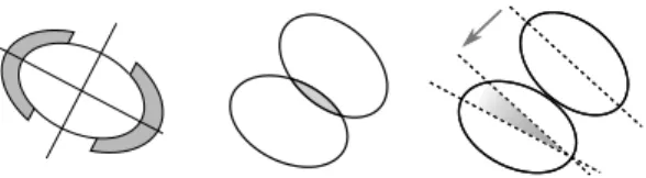
model the overlapping and alignment between objects, (see Figure 1). The aim is to estimate both the configuration❈ and the parameter✌ based on the image ❨. The procedure for building MPPs consists in first initializing and estimat-ing✌, which is currently performed from the null configura-tion and the Stochastic Expectaconfigura-tion-Maximizaconfigura-tion (SEM) al-gorithm [3], and then extracting the objects by simulated an-nealing [see 4, Chapter 7 and references therein]. However, the price to pay to get a fine extraction is a large computational time. Indeed, in practice, it already takes several minutes for an image of size✷✼✺ ✂ ✸✽✺ px [5]. It would thus take a very long time to run it on full Pleiades images.
The computational cost of MPPs could be greatly reduced if it started with a coarse initial configuration instead of the empty one. This is the reason why, in this work, we con-sider a different approach for the initialization of the config-uration. This approach consists in representing the image as a sum of convolutions between a small image with one single object and a highly sparse matrix with non-zero entries cor-responding to Dirac delta functions defining the positions of objects. Our approach thus relies on two main components: first, the construction of a dictionary containing representa-tive instances of a proxy of the object with different rotations and scales; then, the determination of the non-zero entries of the matrix associated with each dictionary element. This lat-ter component is based on sparse optimization problems, with e.g.an❵✶[6] or a log-sum penalty [7]. The complexity of the problem is linear with the number of pixels in the image mul-tiplied by the number of atoms in the dictionary, which can be very large even for medium-size images. Hence, we propose to use an active set algorithm in order to solve efficiently this
Fig. 1. Representations of the data (left), overlapping (mid-dle) and alignment (right) terms used in the MPP model (1).
problem, in a similar fashion as in [8]. The problem we ad-dress bears resemblance to the convolutive non-negative ma-trix factorization as described in [9, 10]. The main difference is that, in this work, we essentially focus on the sparse ap-proximation stage and on devising an algorithm able to re-cover very efficiently in a very high-dimensional setting the few active variables.
The remainder of the paper is organized as follows. Sec-tion 2 exposes the methods currently used for initializaSec-tion and estimation of the parameter of the MPP model. Sec-tion 3 presents our approach based on the resoluSec-tion of sparse optimization problems and the efficient active set algorithm proposed for solving it. In Section 4, we compare the per-formances of two penalties, namely the❵✶ and the log-sum penalties, on a toy image, and we show how the algorithm can be used as an initial configuration for a finer method, such as MPPs, on a real satellite image. Finally, we present some perspectives of future work in Section 5.
2. CONTEXT AND BACKGROUND
The difficulty of estimating the parameter✌ in (1) comes from two facts: first, the setting is unsupervised, so that the un-knowns are both the configuration❈ and the parameter ✌; second, the normalizing constant❝✌ itself depends on the pa-rameter✌, resulting in a difficult optimization problem. In this section, we briefly introduce the methods currently used for the initialization and the estimation of✌. We refer the reader to [2, 5] and references therein for more details.
2.1. Initialization of MPP
In [4, Chapter 7], the initialization is performed as follows. First, a manual over-estimate☞✵of the number of objects in the image is required. This over-estimate can be taken for in-stance as the maximum number of average-size objects that could fit in a rectangle of the size of the image. Then, the tradeoff parameter✌ is obtained by taking the root of the func-tion
☞✵✰
❩
❑☞ ❡①♣❢ ✌❯❞✭✉✮❣✄✭❞✉✮❀
where✄✭✁✮ is the intensity distribution of a Poisson process, ❑ is the compact space corresponding to the image, and the integral corresponds to the average number of objects with
re-spect to a Papangelou conditional intensity for an empty con-figuration❈ ❂ ❀.
2.2. Estimation of the tradeoff parameter
One way to overcome the complexity of the inference prob-lem in unsupervised setting is to use the Stochastic Expectation-Maximization (SEM) algorithm [3], and to replace the likeli-hood (1) by the pseudo-likelilikeli-hood [11] considering indepen-dance between the objects. Starting from an initial value❫✌✭✵✮, the algorithm alternates between approximating the expected likelihood based on a simulated configuration❈✭❦✮for fixed ❜✌✭❦✮, and updating the parameter❜✌✭❦✰✶✮ from Maximum of
Pseudo-Likelihood [2]. The main issue of the SEM algo-rithm is that it is quite long to converge. A slightly faster estimation can be obtained by Stochastic Approximation EM (SAEM) algorithm [12], which takes into account all the sim-ulated configurations in the approximation of the expected pseudo-likelihood. Even so, the estimation step is still long to compute in practice [5].
3. SPARSE OPTIMIZATION FOR OBJECT DETECTION
In this work, we consider a completely different approach for initializing the configuration. We believe it will considerably speed up the estimation step, since it can be started from a good coarse configuration instead of the empty one.
The general idea of our approach is to consider the image as the sum of convolutions of dictionary elements, represent-ing each instance of the object, with Dirac delta functions on the position of the objects in the image. This actually corre-sponds to a sparse linear optimization problem, since we are looking for the highly sparse matrix of positions. In the fol-lowing paragraphs, we first explain the main idea into more details, then we expose our algorithm and, finally, we discuss some techniques to use it in very high dimensions.
3.1. Optimization problem
We first assume that we have a dictionary with atoms❉❦, ❦ ❂ ✶❀ ✿ ✿ ✿ ❀ ❑, of size ❞ ✂ ❞ corresponding to a proxy of the object with different shapes. For an input image❨ of size ♥ ✂ ♠, the problem can be stated as
♠✐♥ ❳✷❘♥✂♠✂❑ ✰ ❦❨ ❳❑ ❦❂✶ ❳❦✄ ❉❦❦✷❋✰ ✕✡✭❳✮❀ (2)
where❳❦is the activation matrix of size♥✂♠ corresponding to element❉❦ of the dictionary,✄ is the convolution opera-tion with zero-padding and conservaopera-tion of the size of❳❦, ❦ ✁ ❦❋ is the Frobenius norm,✡✭✁✮ is a penalty function, and ✕ is the tradeoff between goodness of fit and penalization. This representation is illustrated in Figure 2. Note that the regu-larization term✡✭✁✮ should promote sparsity in the activation
Fig. 2. Representation of an image as a sum of convolutions of activation matrices with elements of the dictionary.
Fig. 3. The matrix ❋ is formed by concatenation of ❑ Toeplitz matrices where each column corresponds to the vec-torized atoms❉❦ at one possible location in the vectorized image. Here, we only show a simple example for an image of size✺ ✂ ✶ with one atom.
coefficients in❳, since these coefficients correspond to the position of the objects on the image. The construction of the dictionary will be discussed in Section 4.
Problem in (2) can be rewritten in the following way: ♠✐♥
①✕✵ ❦② ❋①❦ ✷
✷✰ ✕✡✭①✮❀ (3)
where② is the vectorized image of length ♥♠, ① contains all the vectorized activation matrices❳❦,❦ ❂ ✶❀ ✿ ✿ ✿ ❀ ❑, con-catenated in one single vector of size♥♠❑ and ❋ is a block Toeplitz matrix that corresponds to the convolution, as dis-played in Figure 3. In this work, we choose to regularize① with a component-wise sparsity promoting term such as an ❵✶-norm [6], corresponding to✡✭①✮ ❂ ❦①❦✶, or a more ag-gressive non-convex regularization term such as the log-sum penalty✡✭①✮ ❂P♥♠❑✐❂✶ ❧♦❣✭✶ ✰ ❥①✐❥❂✒✮ [7].
3.2. 2D active set algorithm
One particularity of problem in (2) is that it is both high di-mensional and extremely sparse. For instance, for an image of size✶✵✷✹ ✂ ✶✵✷✹ with ✶✺ dictionary elements, and contain-ing several hundreds of objects, say◆, we need to recover only◆ non-zero entries in ❳❦out of✶✺ million components. Therefore, it is crucial to use a very efficient algorithm that takes this extreme sparsity into account in order to obtain the solution in reasonable time.
In [8], the authors considered an active set algorithm for solving extremely sparse nonconvex optimization problems.
Algorithm 1 2D-sparse optimization (2D-SO) - Input:❨, ✭❉❦✮❑❦❂✶
- Init.: ⑦❨ ❂ ✵ (reconstructed image) ❋ ❂ ❬ ❪ (active elements)
1: repeat
2: ❘ ✥ ❨ ❨ % Compute residue⑦ 3: ❈❦✥ corr2✭❘❀ ❉❦✮ % Correlation ✽❦ 4: ✐❀ ❥❀ ❝ ✥ ❛r❣ ♠❛①✐❀❥❀❝❈✐❀❥❀❝
5: ❋ ✥ ❬❋ im dic✭✐❀ ❥❀ ❉❝✮❪ % add new active element 6: ① ✥ Solve Problem (3) with current active elements ❋ 7: ❨ ✥ reshape✭❋①✮ % Update reconstructed image⑦ 8: until stopping criterion is met
Their approach is of particular interest in our case as it allows the use of nonconvex regularization terms that improve spar-sity. The main idea behind an active set is to iteratively solve the problem on a small subset of active variables. The subset of variables is updated at each iteration by adding the variable that most violates the optimality conditions.
We propose to adapt this algorithm to the context of image processing as shown in Algorithm 1. First we want to empha-size that we can take advantage of the convolution in order to have efficient computations of correlations (Line 3 in the al-gorithm). The inner problem (Line 6) is solved on a restricted number of active positions and with a sparse matrix❋ con-taining in each column (im dic✭✐❀ ❥❀ ❉❝✮), a vectorized sparse
image with a unique dictionary element at position✭✐❀ ❥✮ in the image. As in [8], the inner problem is solved by using a proximal gradient descent method, such as FISTA [13] for the❵✶-penalty and GIST [14] for non-convex ones. Next, we discuss several strategies that have been performed in order to scale the proposed algorithm to extremely large scale opti-mization.
3.3. Strategies for large scale optimization
First, step 3 in Algorithm 1 consists in computing a 2D in-tercorrelation between the residue❘ and each of the dictio-nary elements❉❦. This step requires♠♥❞✷ operations for dictionary elements of size ❞ ✂ ❞ if performed directly or ✷♠ ❧♦❣✷✭♠✮♥ ❧♦❣✷✭♥✮ if performed in the Fourier domain. In our applications, objects are typically small with respect to the image and a direct computation leads to a computational com-plexity linear in the number of pixels in the image. Moreover, this step is a typical case of embarrassingly parallel computa-tion as the correlacomputa-tions can be computed in parallel for each dictionary element.
Second, we use in the algorithm what is known as a warm-starting trick: the solution at a given iteration is given as ini-tialization of the inner problem (line 6) for the following iter-ation. The inner solver being implemented by a gradient de-scent, the algorithm converges in a few iterations to the new solution. Another trick that allows faster convergence is to
Objects in active set New added objects
Connected component
graph Cluster 1
Cluster 2
Parameters to re-optimize Cluster for parallel optimization
Fig. 4. Illustration of the impact of new added objects in a current active set of objects (left). Only a subset of the active variables has to be updated (in green) and this update can be performed in parallel for several connected component clus-ters (right).
add multiple variables to the active set at each iteration. When the number of objects in the image is important, an active set algorithm requires a lot of iterations. When the variables are added by batch, lines 4-5 are executed several times before solving the problem line 6. Hence, the final number of active set iterations can be greatly decreased as discussed in [8].
Finally we propose to use the structure of the image model and the fact that the objects are of limited size to further im-prove speed through a parallel version of the optimization (line 6). First, one can see from the left part of Figure 4 that, when new active variables are added (in red) to the optimiza-tion problem, the corresponding objects have a limited impact on the objects located far outside a certain range. This sug-gests that the re-optimization at line 6 of the algorithm can be exactly solved only on a subset of the current active variables, leading to a significant decrease in computational cost. The subset of parameters to be re-optimized can be obtained sim-ply by using an efficient algorithm on the connected compo-nent graph of the objects as described in [15]. An additional benefit of this approach is that all the connected components in the graph (black clusters illustrated in the right part of Fig-ure 4), can be solved independently, allowing a parallel im-plementation of the re-optimization line 6 in the algorithm.
4. NUMERICAL EXPERIMENTS 4.1. Generated images
In this paragraph, we compare the performances of the❵✶and the log-sum penalties for a detection task in a toy image where we know exactly the position and shape of the objects. The aim is to investigate the benefit of non-convex penalties over convex ones.
The study was driven as follows. First, we built the dic-tionary from 15 rotations of a truncated 2D-Gaussian distribu-tion, as displayed in the top-right part of Figure 2. Then, we created a✶✵✷✹ ✂ ✶✵✷✹ image by placing randomly over the image 10 objects per atom of the dictionary, and we added
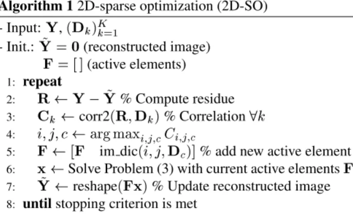
Fig. 5.✶✵✷✹ ✂ ✶✵✷✹ noisy toy image (left), and zoom (right).
a Gaussian noise with variance✛✷ ❂ ✿✵✺. One example of generated image is displayed in Figure 5 and contains 150 objects.
We run the algorithm 2D-SO (see Algorithm 1) with the ❵✶and the log-sum penalties and computed four measures of performance along the regularization path (for a varying✕). The first three measures are based on the F-score, defined by
F-score❂ ✷❚P ✷❚P ✰ ❋P ✰ ❋◆❀
where❚P (true positive) is the number of pixels correctly es-timated as part of an object,❋P (false positive) is the number of pixels that have been incorrectly estimated as part of an ob-ject, and❋◆ (false negative) is the number of pixels that have been incorrectly estimated as part of the background. The F-score thus gives an estimation of the detection rate: the closer to 1, the better the detection is. We computed the F-score on three different matrices: first, for the full image, measuring the overlap between the binary result image and the ground truth; then on the true and reconstructed❳ which measures how well are estimated both position and shape of the objects; and finally, for the position only, thus measuring how well the position of the objects can be recovered, regardless of which dictionary atom is activated. We also computed a fourth mea-sure of quality, namely the mean-squared error between the true matrix of activation and the estimated one.
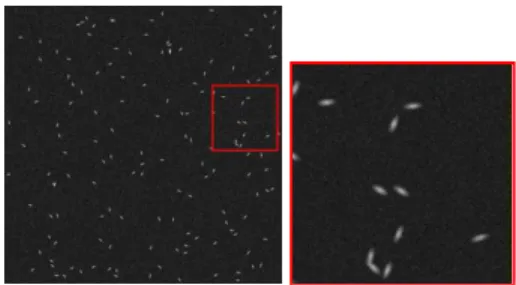
Figure 6 shows the evolution of these four measures as a function of the number of activated objects when varying the regularization parameter✕. The results are averaged over 20 draws. First, note that, between 90 and 170 objects activated, the performances of the log-sum penalty are better than that of the❵✶penalty, whatever the measure. Outside that range, it has equivalent or lower performances. Also, the best F-scores (closest to 1) and MSE (closest to 0) of the log-sum penalty are obtained for 150 activated objects in average, which is ex-actly the number of objects in the toy image. On the other hand, for the❵✶penalty, the best results are obtained between 200 and 270 objects. These results highlight, in the detection problem, the well known issue of the❵✶penalty’s bias, result-ing in poor performances for a small number of objects de-tected and in good performances when the bias is decreased, that is, when more objects are activated. Finally, the perfor-mances in F-score for the full image and for the positions are
0 200 400 600 0 0.5 1 nb activated F − s c o re ( im a g e ) 0 200 400 600 0 0.5 1 nb selected F−score (X) 0 200 400 600 0 0.5 1 nb activated F − s c o re ( p o s it io n ) 0 200 400 600 0 0.5 1x 10 −5 nb activated MSE
Fig. 6. Comparisons of performance of the❵✶ (dashed line) and the log-sum (solid line) penalties, in F-score for the full image (top left), for the positions and shapes (top right), for the positions only (bottom left), and in MSE (bottom right), averaged over 20 draws.
very good, close to one at the optimum, which means that both penalties are able to recover the right position of the ob-jects and a shape at least close to the true one. However, the results in terms of F-score for both the position and the shape are less satisfactory and seem to show a difficulty of the algo-rithm to detect the correct rotation for a given position.
In order to illustrate the temporal complexity of our ap-proach, we ran the algorithm on a✹✵✾✻ ✂ ✹✵✾✻ image con-taining✹✽✵ objects. The optimization with LSP regularization took✻✿✵ min on a computer with 30GB RAM for estimating a sparse vector of size 2.51✂✶✵✽.
4.2. Boat detection on real images
In this paragraph, we apply our algorithm to the problem of boat detection in satellite images of harbors. The original im-age is part of a satellite imim-age, of size✷✼✺ ✂ ✸✽✺. As the objects all have the same orientation, we fixed it to✵✿✻✙, both in the MPP model and in 2D-SO. Also, in the MPP model, boats are approximated by ellipses. Hence, we generated a dictionary of binary ellipses with different scaling so as to better fit the discrepancy in boat size.
In order to compare the performances between the❵✶and the log-sum penalties, we tuned the penalty tradeoff param-eter ✕ in (2) so as to activate a similar number of objects, as shown in Table 1. The table also shows the number of non-overlapping objects obtained after a post-processing step keeping the boats with highest activation coefficient, the F-score for the full image compared to a ground truth, the num-ber of steps for the algorithm to reach convergence, and the computation time. For a similar number of objects, it is clear
❵✶ LSP Activated objects 712 713 Non-overlap. objects 424 489 F-score (image) 0.71 0.77 Steps 77 78 Time (sec) 8.8 11.7
Table 1. Comparison between❵✶and log-sum penalties for a dictionary with 6 scales.
Method Final F-score Estimation time (min.) NC-SEM ✼✵✿✹✷ ✭✶✿✷✵✮ ✽✿✶✾ ✭✷✿✵✶✮ NC-SAEM ✼✵✿✶✹ ✭✵✿✾✾✮ ✼✿✸✶ ✭✷✿✺✷✮ 2D-SO-SAEM ✼✸✿✻✼ ✭✵✿✾✾✮ ✹✿✷✹ ✭✶✿✸✺✮ Table 2. Comparison of performances in F-score for the im-age and in computational time of the estimation step when MPPs are initialized with the null configuration (NC) and with our algorithm (2D-SO). The results are given in average over 50 examples with standard deviations given in parenthe-sis.
that LSP is more accurate as it has less overlapping objects and a better F-score than the❵✶penalty. It still misses some objects, the correct number being 615, but the computation time is very good and promising.
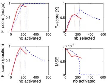
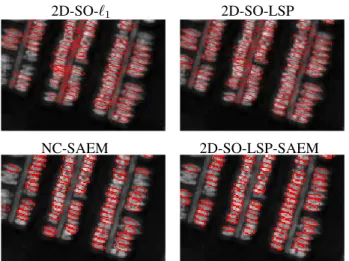
Figure 7 displays the configurations obtained from the es-timation step with SAEM (top right), and from the 2D-SO algorithm with the❵✶ and the log-sum penalties (top row). For 2D-SO, the images displayed result from after a post-processing step removing overlapping objects where we keep the objects having the biggest activation coefficient. From this figure, it appears that the detection with the❵✶ penalty is not as good as the one with LSP, since it has many spaces where no objects were detected or many objects still overlap. This suggests that running SAEM from an initial configura-tion obtained with 2D-SO instead of the null configuraconfigura-tion might speed up the estimation step and improve the quality of the estimation, which is confirmed by the results in Table 2. Indeed, the estimation step is performed almost twice faster, while the gain in detection rate is of more than✸✪. The big difference of computation time between MPP and 2D-SO is mainly due to the fact that MPP tests for many small random perturbations of the objects’ shape to find the one that best fits the image. Hence, it results in a fine estimation of the pa-rameters of each ellipse. Note that the detection rate is lower at the end of MPP than at the end of our algorithm. This is a side effect of the parametrization of MPPs fixing the maxi-mum size of the boats, which can still be optimized. Indeed, the MPP program removes the larger boats, while it greatly improves the shape of the smaller boats (see bottom images of Figure 7).
2D-SO-❵✶ 2D-SO-LSP
NC-SAEM 2D-SO-LSP-SAEM
Fig. 7. Detail of the configurations obtained from 2D-SO with❵✶penalty after post-processing (2D-SO-❵✶), and from 2D-SO with log-sum penalty after post-processing (2D-SO-LSP), from MPP with null configuration (NC-SAEM) and from MPP initialized with the results of 2D-SO-LSP (2D-SO-SAEM). Best seen in color.
5. CONCLUSION AND FUTURE WORKS In this work, we presented an original way of treating the problem of detecting objects in an image as a sparse opti-mization problem. We proposed an efficient algorithm based on an active set strategy that is able to solve the problem in millions of dimensions. The numerical study confirmed that nonconvex penalties result in a more aggressive sparsity and a more accurate detection, and should be preferred over the❵✶ penalty.
The next step of our work is to test the scalability of our method on larger images, and its performances on other types of images, such as astronomical or medical images.In the longer-term, we intend to work on the refinement of the dictionary. Several options seem interesting: an interpolation or a vote to select between different atoms for overlapping objects, which can also be done automatically with the Elitist Lasso [16]; and finally, dictionary learning, where both the dictionary and the activations are estimated simultaneously.
References
[1] M. N. M. van Lieshout, Markov Point Processes And Their Applications, Imperial College Press, 2000. [2] S. Ben Hadj, F. Chatelain, X. Descombes, and J.
Zeru-bia, “Parameter estimation for a marked point pro-cess within a framework of multidimensional shape ex-traction from remote sensing images,” in Symp. Pho-togramm. Comput. Vis. and Image Anal. (PCV), Paris, France, September 2010.
[3] G. Celeux and J. Diebolt, “The SEM algorithm: a prob-abilistic teacher algorithm derived from the EM algo-rithm for the mixture problem,” Comput. Stat. Q., vol. 2, no. 1, pp. 73–82, 1985.
[4] X. Descombes et al., Stochastic geometry for image analysis, Wiley/ISTE, 2013.
[5] A. Boisbunon and J. Zerubia, “Estimation of the weight parameter with SAEM for marked point processes ap-plied to object detection,” in Eur. Signal Process. Conf. (EUSIPCO), Lisbon, 2014, accepted.
[6] R.J. Tibshirani, “Regression shrinkage and selection via the Lasso,” J. Roy. Stat. Soc. B Met., vol. 58, no. 1, pp. 267–288, 1996.
[7] E. Candes, M. Wakin, and S. Boyd, “Enhancing sparsity by reweighted❵✶minimization,” J. Fourier Anal. Appl., vol. 14, no. 5-6, pp. 877–905, 2008.
[8] A. Boisbunon, R. Flamary, and A. Rakotomamonjy, “Active set strategy for high-dimensional non-convex sparse optimization problems,” in Int. Conf. Acoust. Spee. (ICASSP), 2014.
[9] P. Smaragdis, “Convolutive speech bases and their ap-plication to supervised speech separation,” IEEE Trans. Audio Speech, pp. 1–12, 2007.
[10] P. O’Grady and B. Pearlmutter, “Convolutive non-negative matrix factorisation with sparseness con-straint,” in IEEE Int. Workshop Mach. Learn. Signal Process. (MLSP), 2006.
[11] J. Besag, “Statistical analysis of non-lattice data,” The Statistician, vol. 24, no. 3, pp. 179–195, 1975.
[12] B. Delyon, M. Lavielle, and E. Moulines, “Convergence of a stochastic approximation version of the EM algo-rithm,” Ann. Stat., vol. 27, no. 1, pp. 94–128, 1999. [13] A. Beck and M. Teboulle, “A fast iterative
shrinkage-thresholding algorithm for linear inverse problems,” J. Imaging Sci., vol. 2, no. 1, pp. 183–202, 2009.
[14] P. Gong, C. Zhang, Z. Lu, J. Huang, and J. Ye, “A gen-eral iterative shrinkage and thresholding algorithm for non-convex regularized optimization problems,” in Int. Conf. Mach. Learn. (ICML), 2013, vol. 28, pp. 37–45. [15] J. Hopcroft and R. Tarjan, “Algorithm 447: efficient
al-gorithms for graph manipulation,” Commun. ACM, vol. 16, no. 6, pp. 372–378, 1973.
[16] M. Kowalski and B. Torr´esani, “Sparsity and persis-tence: mixed norms provide simple signal models with dependent coefficients,” Signal, Image and Video Pro-cess., vol. 3, no. 3, pp. 251–264, 2009.