HAL Id: hal-01282264
https://hal.inria.fr/hal-01282264
Submitted on 3 Mar 2016
HAL is a multi-disciplinary open access
archive for the deposit and dissemination of
sci-entific research documents, whether they are
pub-lished or not. The documents may come from
teaching and research institutions in France or
abroad, or from public or private research centers.
L’archive ouverte pluridisciplinaire HAL, est
destinée au dépôt et à la diffusion de documents
scientifiques de niveau recherche, publiés ou non,
émanant des établissements d’enseignement et de
recherche français ou étrangers, des laboratoires
publics ou privés.
Multicore SMT scheduling of periodic task systems with
energy minimization
Emilien Kofman, Robert de Simone, Amani Khecharem
To cite this version:
Emilien Kofman, Robert de Simone, Amani Khecharem. Multicore SMT scheduling of periodic task
systems with energy minimization. Workshop on Highly-Reliable Power-Efficient Embedded Designs,
Mar 2016, Barcelone, Spain. �hal-01282264�
Multicore SMT scheduling of periodic task systems
with energy minimization
Emilien Kofman
CNRS, UNS, INRIA Sophia-Antipolis, France Email: [email protected]
Robert de Simone
INRIA, Sophia-Antipolis, France Email: robert.de [email protected]
Amani Khecharem
INRIA Sophia-Antipolis, France Email: [email protected]
Abstract—Energy budget is an intrinsic limitation of mobile electronic appliances such as smartphones or other connected ob-jects. Energy saving is made to compete in modern design against performance optimization. Energy saving mechanisms are usually available (such as power or clock gating, frequency/voltage scaling), but methods to assess their efficiency operate at diverse levels. Either very high, with Excel-like formulas expressing cost functions in systems where applicative dynamic aspects are scarcely present, or already rather low with SystemC transaction-level simulation models in which dynamic abstractions of both actual applicative code and underlying Operating System and instruction-set architecture are needed. In the present paper we describe an intermediate level practical technique for exploiting power/performance ratio information with mathematical solving methods, such as Sat Modulo Theories (SMT) and Constraint Programming. The goal is to get estimation results and opti-mization proposals at the medium intermediate range, where application use cases have dynamic behaviors, but at a level much coarser than instruction-level code or even algorithmic function block. We present modeling and benchmark results illustrating our approach on a simple big.LITTLE-type architecture.
I. INTRODUCTION
In this work we consider an offline scheduling problem of periodic tasks on heterogeneous multicores resources. Energy minimization for this problem is NP-Hard in the strong sense [1]. There exist scheduling heuristics (sometimes energy-aware) that try to get around the complexity. They often stick to a very specific power, task or resources models. Instead, we try to tackle the complexity and find a description of the scheduling problem that is concise enough such that state of the art solvers are able to handle non trivial instances. We give some insights of the scalability of SMT solvers for this type of scheduling problems, and a more extensive study can be found in a previous work [2]. System-level designers usually describe a limited set of tasks such as basic linear algebra routines or spectral methods and try to fit them of the architecture. Our approach provides an automatic load-balancing and offline scheduling technique for those coarse blocks that can also be used as a back-end for code generation. However, automatic code parallelization with thousands of parallel sections is out of the scope of this paper.
In order to better understand the energy/performance bal-ance we get realistic values from an ARM big.LITTLE
This work was partly funded by the French Government (National Research Agency, ANR) through the Labex UCN@sophia (“Investments for the Future” Program #ANR-11-LABX-0031-01).
platform equipped with power sensors and we validate our modeling decisions by experimentation on this prototype. Then, with a model of the power consumption of the resources, we show the effects of two power saving techniques on the scheduling problems search space. The first technique is known as Dynamic Voltage and Frequency Scaling (DVFS). It consists in changing the speed of the resources dynamically, the higher the speed the higher the instant power. Power gating consists in shutting down some areas of a chip and thus some resources, which saves more energy than if it was idle. It is known that the recent OS schedulers do not make efficient use of those techniques, and sometimes even misuse them[3], causing spurious energy loss. We try to show on some example problems that in either case it should still be possible to find a schedule that meets all the deadlines.
Section II describes the modeling problem and the trans-formation to a constraint programming problem. We use a synthetic running example to demonstrate the methodology. Section III gives some evidence that the modeling is realistic, and section IV compares our work to other approaches.
II. MODELING
In this work we consider periodic task systems and we show how to transform them into finite state verification problems. The approach allows to study other types of task systems, such as Dynamic Acyclic Graphs or independent tasks. It also allows to mix both with very little effort. Finding heuristics for every specific problem would be a much larger time investment, hence why we study this methodology. Moreover, our approach allows to produce optimal schedules for small but realistic problems, which could then be used for meta-compiling. Of course the optimality holds assuming that the time and power models are exact, which is why we also discuss them.
A. Description of the scheduling problem
The studied system is made of a set of periodic tasks τ where deadlines equal periods. This means that a task is due within its period. We model the architecture as a set of exclusive heterogeneous resources R with variable speed.
The resources are exclusive, which means that at a given date in time, both resources are either idle or executing only one task. We call this problem the task allocation or task
mapping problem. Unless it is preempted, a task occurrence thus executes only on one resource.
The resources are allowed to change their speed when a task ends or starts. The higher the speed, the higher energy consumed. We call those variable speeds frequency states, or Operating Points (OPP). An OPP is a tuple of voltage and frequency that is withing a guarantee range for a given chip. Although there exist an infinite valid number of voltage and frequency tuples, the typical operating systems often allow only a finite subset of tuples. Sometimes, the user is asked to chose between those OPP which are often no more that a few, for instance: Maximum performance, Low energy, and Balanced.
1) Logical and physical time: Because the tasks can run at
different speeds, their associated cost is a number of cycles
tlt which we call a logical time duration. If task t runs at opp
O with the associated voltage and frequency: V and f , then
its duration will be tpt = tflt which we call a physical time
duration.
2) Resource heterogeneity: The “big.LITTLE” platform is
an example of heterogeneous architecture, with Cortex-A7, Cortex-A15 CPU cores and a GPU core. Even though both CPU cores implement the same instruction set (Armv7-A) and thus can run the same binary file (which allows task migration), the number of cycles per instructions is different for both cores, which is why we call them heterogeneous. The Dhrystone benchmark [4] illustrate this heterogeneity and reports 1,9 DMIPS/MHz for A7 and 3,5 DMIPS/MHz for A15. The heterogeneity is specific to each task, depending on what the task does, for instance integer arithmetic, or floating point operations, or if the task is memory bound.
B. Transformations
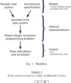
In order to submit to the solver something that it will be able to handle, we need to apply successive transformations to the problem. Figure 1 shows the workflow of our approach. Technically speaking we use a textual concrete syntax for the models, python scripts for the intermediate transformations, z3 (with the python API) for the search, and then gnuplot for visualizing the results.
1) Periodic to bounded time: In order to check the problem
for satisfiability, we need to find a finite interval of time in which the number of occurrences of the tasks will be repeated.
Let tpbe the period of task t, we call this interval a macrocycle
and we calculate it as the least common multiplier of the periods:
M = LCM (tp | t ∈ T asks) (1)
For each task we thus instantiate Mt
p number of instances, with
proper time appearance ta and deadlines td such that the task
occurrence has to occur within its period. We thus transform the periodic scheduling problem to a non periodic one that models the behavior of the latter over one macrocycle.
2) Bounded time to Mixed Integer Programming: In order
to better leverage the fact that in this problem the costs are often related to each other, we make extensive use of
bounded time task system
Mixed integer constraint programming problem Periodic task system Architecture specification Tasks allocations and schedules Models
- human readable syntaxes - quantities with units
Internal representations
Output
- json
- quantities with units
Fig. 1. Workflow TABLE I
TASK COSTS(LOGICAL TIME,INMEGACYCLES) A B
big 30 15 little 35 20
the “Rational” type of symbolic mathematical programming packages (such as “sympy”) in order to reduce the state space of the problem. This methodology allows to detect implicit equalities [5] when they occur and to let the solver know about them.
Given the example of Figure 2 with the costs of Table II, we calculate the associated rational time cost (we give the evaluated float such that we can relate them, but we use the
fraction within the tool), for instance 1003 s for task A running
at 1GHz, 1403 s if it runs at 1.4GHz and so on. Let the timestep
of the scheduling problem be the GCD of those costs:
dt = GCD(tpt| t ∈ T asks) (2)
dt is 84001 s in this example: we can then find the smallest
integer cost presented in Table II. This ensures the smallest but yet complete search space for the scheduling problem. We then submit the mixed integer programming problem to the SMT solver. For the sake of readability we do not introduce another notation for the integer physical time, but instead we
use the same tpt.
The following variables are the exhaustive set of variables for one task of the problem:
• tstart the physical time at which task t starts
• tmap the associated resource of task t
• topp the associated opp of task t
We also define the intermediate variables tptand tstop. tpt is
determined by a combination of tmap and topp (see Table II),
and tstop, is determined by tstart and tpt (see the constraints
thereafter). taand tdare the interpreted constants respectively
for the task appearance and the task deadline. All the
time-related variables are physical time integers. On contrary, tmap
TABLE II
RATIONAL AND INTEGER TIME COSTS
OPP A B Rational (s) Int Rational (s) Int big 1 GHz 1003 (0.030) 252 2003 (0.015) 126 1.4 GHz 1403 (0.021) 180 2803 (0.011) 90 2 GHz 2003 (0.015) 126 4003 (0.008) 63 little 0.6 GHz 1207 (0.058) 490 301 (0.033) 280 1 GHz 2007 (0.035) 294 501 (0.020) 168 1.4 GHz 401 (0.025) 210 701 (0.014) 120
The following equations are the (non exhaustive) set of constraints that we submit to the solver:
∀t ∈ T asks :
tstop = tstart+ tpt
tstart>= ta
td >= tstop
...
∀ distinct tuple (t, u) ∈ T asks2
tmap= umap =⇒ (tstop<= ustart)⊕(ustop<= tstart)
...
3) Non-preemptive to preemptive: The resources are
inter-connected with a Crossbar (that can be shared) of a given speed. In this model of tasks, communications occur only when a task is preempted and migrated. We also experiment with preemptive problems and thus we model the cost of preemption with a message over this Crossbar. The message corresponds to the cost of saving the previous state of the task and restoring it in the local memory of the resource that resumes the task.
[] lowest level of unshared mem, cache L1 in the case of the bigLittle.
We recall that in order to identify a valid steady state schedule we study the problem over one macrocycle, thus the tasks with small periods are duplicated over the time of the macrocycle. This means that two occurrences of this task could run on two different resources. In that case we consider that there is no communication cost because the state of the task when it ends or starts is known at compile time, thus the state of the memory when the task starts or stops can be anticipated. We distinguish this from preemption in that in the case of preemption, the receiving resource will need the state of the preempted task is order to resume it. For instance this state may contain data that has been submitted to the task when it started.
We implement the transformation to preemption by trans-forming the finite states scheduling problem into the same class of problems, with each task and associated cost divided a given number of times. The smallest and sufficient number of preemptions is a disputable topic known as “limited preemp-tion” [6] which we do not address here. However finding this smallest and sufficient number of preemptions is interesting
because the solver time grows fast with the number of tasks. In this work we experimented only with a small amount of preemption.
C. Power model
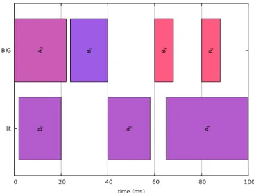
It is already possible to submit to the solver a set of con-straints that allow to solve the previously described scheduling problem. What we obtain is a schedule that satisfies all the deadlines of the tasks. Figure 2 gives an example of schedule for two tasks of arbitrary costs. Task A has a period of 50ms and task B has a period of 20ms which makes the macrocycle equal to 100ms. This means that in order to identify a steady state behavior we have to study the scheduling problem over 100ms, which means over 2 occurrences of A, and 5 occurrences of B. Each occurrence is able to run at a different speed (the color code is such that a red task is executed at a high-power OPP), and on a different resource, which the solver chooses such that each occurrence is able to run within its period. lit BIG 0 20 40 60 80 100 B4 A1 B0 A0 B2 B3 B1 time (ms)
Fig. 2. Example schedule with satisfied constraints
Because we asked only for satisfiability, we can see that the solver did poor choices when it comes to energy opti-mization. In order to get an energy optimized schedule, we need to model the fact that high speed OPPs are more energy consuming.
On contrary to task costs and frequencies, and because we measure the energy related data, the energy related character-istics of the problem may not be closely related to each other, which is why we model their quantities with a regular float type.
1) DVFS: Given the OPP o = (V, f ) of a resource r, we
can calculate its instant power with the following model:
P (r, o) = Cr· V2· f · A (3)
The variables and their dimensions are listed below:
• Cr Farads: the model capacitance of the CPU (roughly
• V Volts: the voltage of the current operating point
• f Hertz: its associated frequency
• A dimensionless: An activity factor that models the
average number of bit flips that the task will cause on the resource. Although it is specific to each pair of task and resource and often approximated to 1. We distinguish only the idle task, with an activity factor of 50 percent as the experiment presented in Figure 4 suggests.
Section III-A shows how we found realistic values for Crand
activity factor on the big.LITTLE platform.
2) Power gating: We consider the static power of the
resources but we do not consider that the resources are able to turn on and off during the macrocycle. If at least one task has to execute on one resource, then this resource is always on in the steady state system. Then it will be idle in its spare time, at its lowest power OPP but with non-zero power consumption. As the reader understands, the instant power of the system depends on time because the resources are allowed to change their operating point in time. The activity factor can change in time as well because the tasks do not employ the micro architecture in the same manner. Given the instant power P (R), the energy with a dimension of W atts·seconds namely J oules is thus calculated for each resource r:
Ea(r) = Z t=end t=0 P (r) dt (4) = Cr· Z t=end t=0 V2· f · A dt (5)
Because we distinguish only idle and active tasks, we can
consider only two activity factors: Aidleand Aactive. If we set
Aactiveto 1, then Figure 4 suggests that Aidle is about 50%.
Let to be the opp for task t, this means that each resources r
running at opp o consumes:
E(r, o) = X t∈T asks|to=o ·Cr f · V 2 o · f E(r, o) = X t∈T asks|to=o Cr· Vo2
Let Orbe the set of OPPs of resource r, the energy consumed
by the tasks running on r is:
Ea(r) =
X
o∈Or E(r, o)
We call that quantity “active” energy consumption.
Finally let Pidle be the idle instant power of the resource,
the idle energy can also be expressed as a discrete sum:
Ei(r) = Pidle· (M −
X
t∈T asks|tmap=r
tpt) (6)
Thus, the consumed energy of the system is:
E = sum(Ei(r) + Ea(r) | r ∈ R) (7)
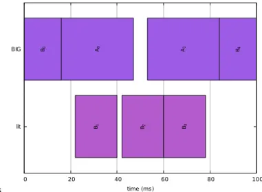
That E is what we try to minimize. Figure 3 shows the solution to the same problem presented in Figure 2, but with an optimized energy consumption.
s lit BIG 0 20 40 60 80 100 A0 A1 B4 B0 B1 B2 B3 time (ms)
Fig. 3. Example schedule for the same problem as figure 2 and with optimized energy consumption
3) Temperature modeling: In this study we do not consider
the effect of temperature. We believe that (depending on the length of the macrocycle) we can study this problem at another time scale and we are able to find a stationary behavior that also keeps the chip at a constant temperature. Moreover, the most well known technique that protects the chip from burning is thermal throttling, which consists in inserting cycles of “no operation” into the pipeline of the micro-architecture instead of running the actual software. Because it is very hard to control how much and when throttling is applied, we consider that in order to retain the predictability hypothesis, we should be able to avoid raising the temperature to that point. Moreover, because thanks to our power model we know how much power the computing will drain, and because we know that this power will mainly be dissipated as heat, the embedded system designer can then scale its cooling device accordingly.
III. RESULTS
A. Power model validation
Because the big.LITTLE prototype that we use is equipped with power sensors we performed small experiments in order to build our models out of realistic data. Figure 4 shows the measured energy for active and idle states of the big resource. We conducted those experiments using the tools “cpufreq-set”, “stress”, “taskset” and “lm-sensors”. We conducted the same for the little resource in order to obtain realistic instant power values.
Out of curiosity, what we also found is that the instant powers of the little core at high frequencies can reach the same magnitude (and even higher)+ than the instant powers of
the big core at low frequencies. For instance Plittle,800M Hz<
0 0.2 0.4 0.6 0.8 1 1.2 1.4 1.6 1.8 2 0.2 0.4 0.6 0.8 1 1.2 1.4 1.6 1.8 2 P o w e r (W ) Frequency (GHz) idle stressed ratio model
Fig. 4. power consumption under different OPPs
the resources are heterogeneous, the equality does not hold for energy consumption, thus it’s an inexact shortcut to decide the task assignments based on those relations only. And even though we calculate the energy cost of each task on each resource, it could happen that because of deadline constraints, it might be necessary to choose not the lowest energy con-sumption resource and OPP for that task occurrence.
B. Scalability of the approach
The main drawback of this approach is obviously its scala-bility. One can imagine that a naive exhaustive search would have an exponential complexity in number of tasks, resources, and OPP. The recent improvements in the domain of SMT solvers [7] allow to scale up to tens of tasks and resources. However we emphasize that the number of tasks is not the proper metric to qualify the scalability of such problems [2]. Moreover we consider that in the domain of embedded devices it is realistic to think that the problems will exhibit only a small number of task occurences. Hopefully it will be small enough such that an SMT solver can handle it.
We also find that the performance of the solver depends a lot on the load of the system: if the schedule is very tight, it is likely that the solver will need much more time in order to find it. However it may be very fast at detecting unsatisfiable problems or problems where there is a lot of spare time. This insight is consistent with the results obtained in previous work [2], in which the load is identified as one of the main noticable criteria for scalability. In this work we also experiment with different types of task models, such as directed acyclic graphs of tasks, and we show that depending on the shape of the graph (high depth or high breath) we can expect a different scalability in number of tasks.
C. Example sound solver decisions
In this section we show that our modeling is precise enough such that the solver investigates the sound decisions that an human would have been finding if he/she did the math
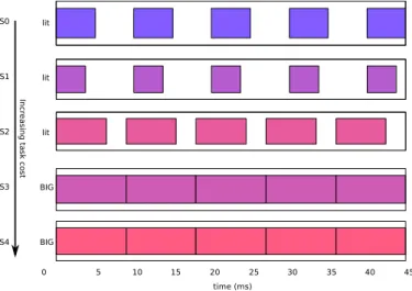
him/herself. For instance when all the problem can be solved on the low-power resource, at a low-power OPP, the solver obviously returns this solution. Figure 5 gives the example of the different schedules produced for only one periodic task (over a few macrocycles). Increasing the cost of this task successively changes the schedule to higher OPPs (e.g.
schedules S0 to S2), then to the big resource (S2 to S3) and
then again to the higher OPP of the big resource (S3 to S4).
lit 0 5 10 15 20 25 30 35 40 45 time (ms) lit lit BIG BIG S0 S1 S2 S3 S4 Incr
easing task cost
Fig. 5. Schedules found when increasing task cost
D. Effects of preemption
For very tight problems, we were able to show that non preemptive schedules are unsatisfiable while preemptive schedules are satisfiable. This happens when the tasks have to share a high performance resource that is not high enough such that it could compute both tasks entirely. Because the problems with very fine preemption will not scale very well, this exhibits one of the limitations of our approach. However, because the preempted chunks have to be ordered, preemptions scales better than a set of independent tasks.
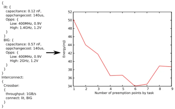
We experimented energy minimization of preemption prob-lems with two tasks of the same heterogeneous cost (15MCy and 30MCy resp. on little and big resources). We successively raise the number of preemption points for each task. Figure 6 shows the model with the OPP and the results of this exper-iment. We observe that as we expected, the finer preemption levels provide the better energy savings. However we also see that it is not a monotonically decreasing function, which means that we may find a small and sufficient preemption level that minimizes energy consumption.
IV. RELATED WORK
Some specific cases (uniprocessor, two homogeneous pro-cessors ideally connected, ...) admit pseudo polynomial time algorithms [8]. For the general cases instead, the encoding that we use is often considered intractable with no or little investigation. Thus, heuristics are developed for each specific problem which is why the literature is abundant on those topics. Often, known heuristics such as list scheduling [9],
34 36 38 40 42 44 46 48 50 52 1 2 3 4 5 6 7 8 9 Ener gy(mJ)
Number of preemption points by task
Fig. 6. Minimum reachable energy consumption with preemption refinements
Earliest Deadline First, or Rate Monotonic[1] are modified such that they become “energy-aware”. Many of those heuris-tics ignore the idle-state consumed energy, and are simulated in environments that also ignore it. Hence the gain that they report is not realistic [10].
Our methodology is versatile because it allows to change the model or the problem type. However, it could happen than some specific problems (homogeneous resources, uniproces-sor scheduling) also perform better with a slightly different encoding even though there exists an encoding that can handle a very wide range of problems. It is crucial to ensure that the successive transformations are correct. For instance, similar work distributes the rate of the tasks instead of actually doing the scheduling [11]. This has the benefit that the problem is less complex, however in the case of tasks with different periods this model is not exact. The same transformation to a bounded time scheduling problem is applied, but then the model is allowed to distribute the rate of every task all over the macrocycle, which is not the same specification than the original periodic system of tasks. It could be however interesting to split this rate distribution on the basis of the GCD of the periods. This would better model the initial problem (with an additional number of variables, thus an additional complexity) but would still lack the ability to refine the model. For instance adding a preemption cost would not be feasible since the model simply does not allow to know how many preemptions occur.
V. CONCLUSION
We show that the tool is versatile enough such that it can be used to experiment with scheduling problems on realistic architecture models. We were able to easily add refinements to the model such as the cost of an OPP change, or the cost of a task preemption in order to get an idea of their footprint on the scheduling search space. We were able to show that the modeling of the power gating and DVFS energy saving techniques actually translates to specific scheduling decisions. We also show how the models can be further refined such that the search space is reduced but still contains the interesting schedules. We plan to investigate different type
of task models, for instance embarrassingly parallel tasks, or preemption in blocks of variable size (where the size would be a variable for the solver). For instance the experiment presented in Figure 6 suggests that an interesting modeling would be fewer preemption points, but preempted blocks of variable size.
REFERENCES
[1] T. AlEnawy, H. Aydin, et al., “Energy-aware task allocation for rate monotonic scheduling,” in Real Time and Embedded Technology and Applications Symposium, 2005. RTAS 2005. 11th IEEE, pp. 213–223, IEEE, 2005.
[2] R. Gorcitz, E. Kofman, T. Carle, D. Potop-Butucaru, and D. S. Robert, “On the scalability of constraint solving for static/off-line real-time scheduling,” in Formal Modeling and Analysis of Timed Systems, pp. 108–123, Springer, 2015.
[3] E. Le Sueur and G. Heiser, “Dynamic voltage and frequency scaling: The laws of diminishing returns,” in Proceedings of the 2010 international conference on Power aware computing and systems, pp. 1–8, USENIX Association, 2010.
[4] R. P. Weicker, “Dhrystone: a synthetic systems programming bench-mark,” Communications of the ACM, vol. 27, no. 10, pp. 1013–1030, 1984.
[5] P. J. Stuckey, “Incremental linear constraint solving and detection of implicit equalities,” ORSA Journal on Computing, vol. 3, no. 4, pp. 269– 274, 1991.
[6] G. Yao, G. Buttazzo, and M. Bertogna, “Comparative evaluation of limited preemptive methods,” in Emerging Technologies and Factory Automation (ETFA), 2010 IEEE Conference on, pp. 1–8, IEEE, 2010. [7] L. De Moura and N. Bjørner, “Z3: An efficient smt solver,” in Tools and
Algorithms for the Construction and Analysis of Systems, pp. 337–340, Springer, 2008.
[8] H. Aydin, R. Melhem, D. Moss´e, and P. Mejia-Alvarez, “Dynamic and aggressive scheduling techniques for power-aware real-time systems,” in Real-Time Systems Symposium, 2001.(RTSS 2001). Proceedings. 22nd IEEE, pp. 95–105, IEEE, 2001.
[9] R. Mishra, N. Rastogi, D. Zhu, D. Moss´e, and R. Melhem, “Energy aware scheduling for distributed real-time systems,” in Parallel and Distributed Processing Symposium, 2003. Proceedings. International, pp. 9–pp, IEEE, 2003.
[10] S. Saha and B. Ravindran, “An experimental evaluation of real-time dvfs scheduling algorithms,” in Proceedings of the 5th Annual International Systems and Storage Conference, p. 7, ACM, 2012.
[11] H. S. Chwa, J. Seo, H. Yoo, J. Lee, and I. Shin, “Energy and feasibility optimal global scheduling framework on big. little platforms,”