Effets de Champ Ferroelectriques dans des dispositifs à base d'oxydes supraconducteurs HTC

U

P

M

C

–

P

VI

F

P

Ecole doctorale Physique et Chimie des Matériaux

T

HESIS

Ferroelectric Field-Effects in High-T

c

Superconducting Devices

presented by Laura B

-L

to obtain the degree of

Doctor of Philosophy

defended on January, 23

_{2017 in front of the committee:}

Kathrin D

Martin Luther Univesität - Halle-Wittenberg

Referee

Benjamin M

ICMAB-CSIC - Barcelona

Referee

Abhay S

UPMC-IMPMC - Paris

Examiner

Jacobo S

Universidad Complutense de Madrid - Madrid

Examiner

Hervé A

ESPCI-LPEM - Paris

Examiner

Manuel B

Unité Mixte de Physique CNRS-Thales - Palaiseau

Supervisor

I

Unité Mixte de Physique

CNRS-Thales

1 av. Augustin Fresnel

91767 Palaiseau

France

Ecole doctorale Physique et Chimie des

Matériaux

4 place Jussieu

75005 Paris

France

II

Remerciements

Ces années de thèse m’ont énormément apporté sur les plans scientifique et humain. J’ai eu la chance d’évoluer dans un laboratoire exceptionnel, où j’ai pu apprendre des techniques, un savoir-faire et des méthodologies en bénéficiant de l’expérience précieuse de chercheurs et d’ingénieurs brillants et généreux. Je remercie en premier lieu mon directeur de thèse, Javier, qui m’a fait confiance et m’a accompagné jusqu’à la dernière ligne de ce manuscrit en surpassant avec moi les états d’âmes et les découragements inhérents à la recherche expérimentale, et en m’encourageant à aller de l’avant avec détermination.

Je remercie très chaleureusement les personnes qui m’ont formé, Rozenn, Karim, Cécile, Stéphanie, Yves, Victor, Eric… vous m’avez tous transmis beaucoup plus que de simples recettes ou des protocoles. Un grand merci aussi à ceux qui se sont impliqué dans mes travaux, Sophie, Vincent, Steef, Anke, Juan, Lee ainsi que Stéphane Xavier, Christian Ulysse et Maria Varela. Merci pour toutes ces heures passées sur mes – souvent pénibles – petits échantillons !

Je remercie aussi sincèrement ceux qui m’ont accordé du temps pour échanger sur mes résultats, en particulier Jérôme Lesueur qui m’a mis au contact de photons intriqués dès la sortie du berceau et qui a toujours su faire de la place dans son emploi du temps pour de longues discussions sur la physique. Merci également à Nicolas, Denis et Agnès pour m’avoir éclairé dans la compréhension de mes travaux, et surtout à Manuel pour m’avoir accompagné dès mon arrivée.

Merci aussi à ceux qui ont partagé un happy office, une pause déj, un café, une conversation à propos d’un piston ou d’un chassis, un apéro, un karting ou une épopée nocturne avec moi pendant ces longues années, vous êtes trop nombreux pour tous vous citer mais une pensée particulière à Piotr, Sophie et Alice pour être venu me témoigner votre amitié quand mes fractures m’empêchaient de me lever, Flavio, Jason et Karim pour les mégawatts de bonheur partagé sous les ondes une fois que j’étais rétablie, Sophie pour les galops à la fraiche le jeudi matin. Un doux merci aussi à Christine pour ta gentillesse, je te souhaite une retraite heureuse et reposante. Je terminerai par remercier Anne, Frédéric N.V.D. et Frédéric P. pour la direction et la canalisation des forces humaines et administratives au laboratoire, c’est une grande chance de vous avoir à la barre.

J’ai également beaucoup de reconnaissance et d’affection pour ceux qui se sont intéressé à mes travaux en dehors du labo, ma famille pour les réguliers « alors ça avance ? », ou mon papa pour son regard moderne sur la supraconductivité. Claire pour toute les fois où on a emmené notre charrette en dehors des sentiers, Max pour toutes les fenêtres qu’il a ouvert en grand dans mon cœur, et surtout ma maman qui a courageusement lu et corrigé avec amour chacune des lignes de cette thèse. Merci

III

Ferroelectric Field-Effects in High-T

c

Superconducting Devices

Abstract

In this experimental thesis, we fabricated ferroelectric field-effect devices based on high-Tc

superconductors. We grew high-quality epitaxial heterostructures consisting of an ultra-thin (2 to 6 unit cells) film of YBCO and a thin ferroelectric film (BFO-Mn). We fabricated transport measurement microbridges and used a CT-AFM tip to polarise the BFO-Mn outwards or towards the BFO-Mn/YBCO interface. Due to the ferroelectric field-effect, the superconducting properties of the underlying YBCO film were consequently modified. We then used this effect locally in order to design weak links within the microbridges: two regions where the superconducting properties are enhanced are separated by a narrow region where they are depressed. We explored the conditions of existence of a Josephson coupling across this weak link.

In parallel, we fabricated ferroelectric junctions. The barrier is an ultra-thin BFO-Mn film sandwiched between a high-Tc superconducting YBCO bottom electrode and a low-Tc superconducting top

electrode. Both at room temperature and at low temperature, we characterised the transport properties across the barrier and the resistive switching resulting from the polarisation of the ferroelectric barrier.

Keywords

Epitaxy, Ferroelectricity, Field-effect, Hall effect, High-Tc superconductors, Interface, Josephson

effect, Lithography, Oxides, Pulsed Lased Deposition, Piezoresponse Force Microscopy, Superconductivity, Tunnel junctions, Ultra-thin films, Weak-links

IV

Effets de champ ferroélectriques dans des

dispositifs à base de supraconducteurs à

haute T

c

Résumé

Les matériaux ferroélectriques possèdent une polarisation spontanée et rémanente. Lorsqu’ils sont recouverts par une électrode, des charges s’accumulent dans cette dernière, à proximité de l’interface, afin d’écranter la polarisation : c’est l’effet de champ ferroélectrique. Alors que dans les métaux cet écrantage a lieu sur une distance très courte, il s’étend sur une distance nanométrique dans les matériaux moins denses en porteurs comme les oxydes. Or, les oxydes sont des systèmes fortement corrélés, dans lesquels une petite variation du nombre de porteurs (typiquement celle induite par la proximité avec un ferroélectrique) suffit à induire de fortes modifications des propriétés physiques du matériau.

Dans cette thèse expérimentale, nous exploitons cet effet dans un oxyde supraconducteur à haute température critique, l’YBCO. Pour cela, deux configurations sont étudiées :

 En géométrie planaire, un film d’YBCO est recouvert par un film ferroélectrique (BFO-Mn). L’épaisseur du film d’YBCO est du même ordre que sa longueur d’écrantage, de telle sorte que l’effet de champ se propage dans toute la profondeur du film.

 En géométrie verticale, deux électrodes supraconductrices possédant des longueurs d’écrantage différentes sont séparées par une fine barrière ferroélectrique. En fonction de la direction de la polarisation, le profil électrostatique de la barrière est modifié.

La première partie de cette thèse a été dédiée à la croissance par ablation laser pulsée d’hétérostructures possédant les propriétés nécessaires pour ces dispositifs : dans le cas des structures planaires, il a fallu conserver la supraconductivité dans des films de quelques mailles unités seulement ; dans le cas des structures verticales, conserver de bonnes propriétés ferroélectriques dans des films nanométriques. Au terme d’un travail d’optimisation, des hétérostructures BFO-Mn (30 nm)/YBCO (2 à 5 m.u.)/PBCO//STO ainsi que des bicouches BFO-Mn (2 à 5 nm)/YBCO (50 nm)//STO d’une grande qualité ont été fabriquées.

Les procédés de lithographie ont été développés afin de fabriquer des dispositifs permettant d’étudier, dans le premier cas, les propriétés de transport dans le film d’YBCO, et dans le second cas, à travers la barrière de BFO-Mn. Les propriétés ferroélectriques de BFO-Mn sur YBCO ont été caractérisées, mettant en évidence deux résultats majeurs : premièrement, un dipôle électrique permanent est présent à l’interface BFO-Mn/YBCO, favorisant une direction de polarisation par rapport à l’autre. Deuxièmement, la polarisation est stable dans les deux directions, et peut être

V

modifiée dans l’air ou dans le vide, à haute et basse température, au moyen d’un simple scan AFM à pointe conductrice (CT-AFM).

Dans un premier temps, les dispositifs planaires ont été entièrement polarisés dans une direction puis une autre, et les propriétés de transport du film d’YBCO ont été mesurées dans les deux états. L’effet de champ s’est manifesté par une modification de la température critique, de la conductivité et du nombre de porteurs libres dans le film d’YBCO. L’état de basse conductivité (déplétion de porteurs dans le film d’YBCO) est obtenu pour une polarisation du BFO-Mn pointant vers l’interface BFO-Mn/YBCO, en accord avec le fait que dans l’YBCO, les porteurs sont de charge positive.

Dans un second temps, des jonctions de type lien faible ont été définies au sein des dispositifs : le ferroélectrique est polarisé vers la surface sur la plupart du dispositif (accumulation de porteurs dans le film d’YBCO) et vers l’interface BFO-Mn/YBCO sur une fine bande (déplétion de porteurs dans l’YBCO). Les différents régimes de transport ont été étudiés pour différentes températures. Des oscillations ont été observées dans les mesures de magnétorésistance et de courant critique en fonction du champ magnétique, supposément dues à un couplage Josephson de part et d’autre du lien faible.

En parallèle, les dispositifs verticaux ont été mesurés. Dans un premier temps, les propriétés ferroélectriques des films ultra-minces de BFO-Mn sur YBCO ont été étudiées à température ambiante à partir de capacités de 300 nm à 1 µm de diamètre. Plusieurs électrodes supérieures – métalliques et supraconductrices – ont été utilisées, mettant en évidence leurs influences sur les propriétés ferroélectriques des films ultra-minces.

Dans un second temps, des dispositifs verticaux avec une électrode supérieure supraconductrice (MoSi) ont été fabriqués. Les propriétés de transport à travers le film ferroélectrique ont été caractérisées à différentes températures, et après l’application d’une tension DC de plusieurs volts dans le but de polariser le film ferroélectrique. La résistance de la barrière s’est révélée dépendante de la tension de polarisation : un comportement hystérétique à deux états a été obtenu, typique des jonctions tunnel ferroélectriques. Les mécanismes à l’origine de cette électro-résistance, observée uniquement sous la température critique de l’électrode inférieure, sont probablement liés à l’effet de champ ferroélectrique.

Les travaux menés au cours de cette thèse ouvrent la voie pour la réalisation de dispositifs à effet de champ ferroélectrique à base de supraconducteurs, comme la réalisation de jonctions Josephson à paramètres continûment variables (en modifiant l’épaisseur de la région déplétée dans le cas des dispositifs planaires) ou à deux états (en modifiant la direction de la polarisation dans les jonctions verticales).

VI

Contents

Introduction ... 1

I. Generalities ... 3

I.1 Superconductivity ... 5

I.1.1 Historical aspects ... 5

I.1.2 London equations ... 6

I.1.3 The BCS theory ... 8

I.1.4 Ginzburg-Landau theory ... 9

I.1.5 Vortices in High-Tc Superconductors ... 13

I.2 Josephson effect ... 14

I.2.1 Tunnel effect... 14

I.2.2 Josephson effect ... 17

I.2.3 Josephson junction in a magnetic field ... 19

I.2.4 Josephson junctions technology ... 22

I.3 Ferroelectricity ... 24

I.3.1 Symmetry ... 24

I.3.2 Mechanisms of ferroelectricity ... 25

I.3.3 Conduction through ferroelectric oxides ... 26

I.3.4 Ferroelectricity in thin films ... 27

I.4 Materials ... 31 I.4.1 SrTiO3 ... 31 I.4.2 PrBa2Cu3O7-δ ... 31 I.4.3 YBa2Cu3O7-δ ... 31 I.4.4 BiFeO3 ... 32 I.4.5 La1-xSrxMnO3 ... 35 I.4.6 Mo1-xSix ... 35

II. Field-effects in correlated oxides ... 37

II.1 Field-Effect Transistors ... 38

II.1.1 Principle of the Field-Effect Transistor ... 38

II.1.2 Electric penetration depth and carrier modulation ... 39

II.1.3 Oxides field-effect transistors technologies ... 40

II.2 Electrostatic tuning of correlated oxides ... 42

II.2.1 Field-Effect in Colossal-Magneto-Resistance Manganites ... 42

II.2.2 Ferroelectric field-effect transistor: a prototypical model ... 44

II.3 Electrostatic tuning of high-Tc superconductors ... 47

II.3.1 Field-effect and penetration length ... 47

II.3.2 Field-Effect Transistors ... 48

II.3.3 Electric Double Layer Transistors ... 49

II.3.4 Ferroelectric Field-Effect Transistors ... 49

II.4 Some functionalities of field-effect ... 51

VII

II.4.2 Tunable Josephson junctions ... 53

II.4.3 Ferroelectric tunnel junctions ... 54

III. Experimental techniques ... 58

III.1 Growth techniques ... 59

III.1.1 Pulsed Laser Deposition ... 59

III.1.2 Sputtering and thermal evaporation ... 61

III.2 Characterisation techniques... 62

III.2.1 Scanning Electron Microscopy ... 62

III.2.2 Scanning Transmission Electron Microscopy (STEM) ... 63

III.2.3 Scanning Probe Microscopy (SPM) techniques ... 63

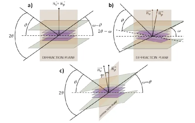
III.2.4 X-Ray diffraction ... 67

III.3 Nano and micro fabrication ... 72

III.3.1 Generalities on fabrication ... 72

III.3.2 Fabrication of planar devices ... 75

III.3.3 Fabrication of planar devices with a gate... 80

III.3.4 Fabrication of vertical devices: matrices of pads ... 82

III.3.5 Fabrication of micrometric vertical devices ... 83

III.3.6 Measurement set-up for electrical characterisation... 84

IV. Growth of epitaxial heterostructures ... 86

IV.1 Epitaxial heterostructures for planar field-effect devices ... 87

IV.1.1 Objectives ... 87

IV.1.2 Preparation of substrates ... 88

IV.1.3 Growth of YBa2Cu3O7-δ ... 88

IV.1.4 Growth of BiFeO3 ... 90

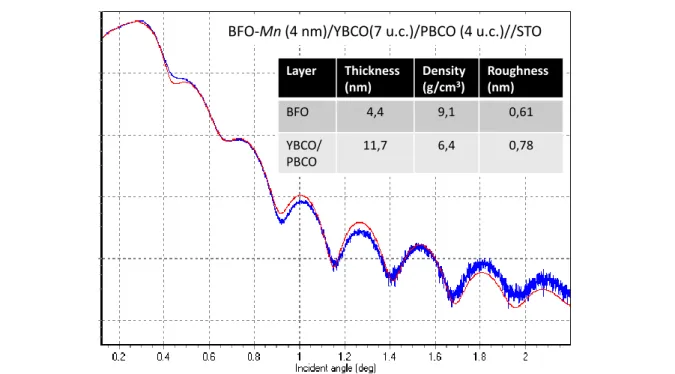
IV.1.5 Properties of optimised BFO/YBCO/PBCO/STO ... 94

IV.2 Epitaxial heterostructures for ferroelectric tunnel junctions ... 101

IV.2.1 Objectives ... 101

IV.2.2 BFO/YBCO in situ heterostructures ... 103

IV.2.3 BFO-Mn epitaxy on YBCO films grown by PLD ... 104

IV.2.4 BFO-Mn epitaxy on YBCO commercial films ... 106

V. BFO/YBCO ferroelectric properties... 110

V.1 Stability of the ferroelectric domains ... 111

V.1.1 Samples not exposed to an O2 plasma ... 111

V.1.2 Samples exposed to an O2 plasma... 114

V.1.3 Asymmetry of the ferroelectric characteristics of BFO films on YBCO ... 115

V.1.3. a) Electrostatic interactions ... 116

V.1.3. b) Pinned ferroelectric layer ... 117

V.1.3. c) Pinned ferroelectric domains ... 118

V.2 Structure of the BFO-Mn/YBCO interface ... 119

V.3 Ferroelectric switching inside a cryostat ... 121

V.3.1 Ferroelectric switching in Helium atmosphere ... 121

V.3.2 Ferroelectric switching at low temperature ... 123

VI. Planar field-effect devices ... 125

VI.1 Field-effect measurements ... 126

VIII

VI.1.2 Electrostatic modulation of the carrier density ... 130

VI.1.3 Experiments with a top-gate electrode ... 133

VI.2 Planar S/S’/S junctions ... 135

VI.2.1 Resistive transition of S/S’/S junctions ... 136

VI.2.2 Voltage-current characteristics of the junctions ... 138

VI.2.2. a) General shape of the voltage-current characteristics ... 139

VI.2.2. b) Cross-over regime from the dissipative to the non-dissipative state ... 140

VI.2.2. c) Voltage-current dependence on the magnetic field ... 141

VI.2.3 Magnetotransport ... 142

VI.2.4 Interpretation of the experimental observations ... 147

VI.3 Conclusion ... 151

VII. Out-of-plane field-effect devices ... 152

VII.1 Room-temperature measurements ... 154

VII.1.1 Description of the set-up ... 154

VII.1.2 Characterisation of Pt/Co/BFO-Mn/YBCO junctions ... 155

VII.1.3 Characterisation of Nb/BFO-Mn/YBCO junctions ... 158

VII.1.4 Characterisation of NbN/BFO-Mn/YBCO junctions ... 159

VII.1.5 Characterisation of MoSi/BFO-Mn/CMO junctions ... 160

VII.2 Low-temperature measurements ... 161

VII.2.1 Characterisation of the junctions ... 161

VII.2.2 Field-effect measurements ... 164

VII.2.3 Conclusions ... 166

VII.3 Conclusion ... 167

Appendix ... 170

1

Introduction

The richness of the phase diagram of many complex oxides is due to their strong electronic correlations. They derive, among other mechanisms, from the competition between localisation – due to Coulomb repulsions – and hopping – due to the kinetic energy – of the carriers. This competition can be tuned by changing electrostatically the carrier density: this is the keystone of Field-Effect Transistors (FETs), widely used in nowadays technology. In these devices, a voltage is applied across a dielectric gate, between a thin oxide channel and a metallic electrode. This tunes the carrier density in the channel, inducing a modification of the conductivity of the latter.

Among them, FETs with a ferroelectric gate raise a considerable interest: these materials possess a spontaneous polarisation. At their boundaries, charges accumulate close to the interface in order to screen the ferroelectric polarisation. The polarisation is remanent: the induced charge transfer remains once the electric field necessary to polarise the ferroelectric in one direction is removed. In this experimental thesis, we use the ferroelectric field-effect to tune the electrical properties of a superconductor. The chosen material is YBCO: because of its low carrier density, the field-effect occurs over long distances in this oxide (typically one nanometre). The superconducting properties, in particular the critical temperature, are consequently modified.

We did not only focus on modifying the electrical properties of a channel, but fabricated superconducting devices based on the ferroelectric field-effect. Superconductors have unique properties; among them, the Josephson effect: this phenomenon results from the coupling of two superconductors across a weak link. It has numerous applications, from magnetometers to RSFQ digital electronics. The aim of this thesis is to open the way to ferroelectric field-effect tunable Josephson junctions, based on high-Tc superconductors. To achieve this, two kinds of devices are

studied:

a) Planar devices in a transistor geometry: a ferroelectric film is grown on top of an ultra-thin superconducting channel. The polarisation is in such a way that the superconducting properties are enhanced on most of the channel, except in a thin band where it is depressed (the weak link).

b) Vertical devices in a tunnel junction geometry: an ultra-thin ferroelectric film is sandwiched between two different superconducting electrodes. The current tunnels through the ferroelectric barrier; depending on the direction of the polarisation, the electrostatic height of the latter is modified.

In the first chapter, one will find a description of the general concepts related to these devices: superconductivity and ferroelectricity, Josephson effect, tunnelling… The ferroelectric field-effect presented in the second chapter, in which a brief review of the different transistors and devices found in the literature is given. Then, the experimental techniques involved in the characterisation and fabrication of the devices are detailed in the third chapter.

2

The first step of the fabrication consists in the growth of high-quality heterostructures combining a ferroelectric film and a superconductor: this is the object of chapter IV. Further characterisation of the interface and ferroelectric properties of our structures can be found in chapter V.

Chapter VI presents the characterisation of the planar devices. In this configuration, the

superconducting film is extremely thin (a few unit cells). The ferroelectric field-effect enhances the superconductivity in most of the channel, except in a thin region where it is depressed. This constitutes a weak link. The boundaries between the three regions are very faded, and the proximity effect is very strong in these kinds of devices. We investigate the signature of a Josephson coupling between the two enhanced regions, in a range of temperature where they are in a superconducting state whereas the depressed region is in a normal state. These devices are conceptually fascinating, as the length of the weak link and the strength of the coupling can a priori be of any size, and reconfigurable ad infinitum.

In the second case, the barrier is the ferroelectric film itself; the preliminary results are presented in

chapter VII. High-Tc superconductor/Ferroelectric/Low-Tc superconductor junctions are studied in

both the normal and the superconducting states. The switching of the polarisation in the ultra-thin barrier and the resulting electroresistance are characterised at different temperatures.

3

I. Generalities

Index

I. Generalities ... 3

I.1 Superconductivity ... 5

I.1.1 Historical aspects ... 5

I.1.2 London equations ... 6

I.1.3 The BCS theory ... 8

I.1.4 Ginzburg-Landau theory ... 9

I.1.5 Vortices in High-Tc Superconductors ... 13

I.2 Josephson effect ... 14

I.2.1 Tunnel effect... 14

I.2.2 Josephson effect ... 17

I.2.3 Josephson junction in a magnetic field ... 19

I.2.4 Josephson junctions technology ... 22

I.3 Ferroelectricity ... 24

I.3.1 Symmetry ... 24

I.3.2 Mechanisms of ferroelectricity ... 25

I.3.3 Conduction through ferroelectric oxides ... 26

I.3.4 Ferroelectricity in thin films ... 27

I.4 Materials ... 31 I.4.1 SrTiO3 ... 31 I.4.2 PrBa2Cu3O7-δ ... 31 I.4.3 YBa2Cu3O7-δ ... 31 I.4.4 BiFeO3 ... 32 I.4.5 La1-xSrxMnO3 ... 35 I.4.6 Mo1-xSix ... 35

5

I.1 Superconductivity

I.1.1

Historical aspects

The study of metals at very low temperatures was for a long time limited by the ability to reach these temperatures. In 1908 in Leiden (Netherlands), Heike Kamerlingh Onnes was able to liquefy Helium gas, allowing his student Gilles Host, three years later, to observe a radical drop in the resistivity of a mercury sample at 4,2 K (Figure ‎I.1) [1]. Other metals such as Tin, Lead or Aluminium, behaved the same way, reaching resistivities so small that they would always be beyond the sensitivities of the measurement devices. After this first discovery of superconductivity, Meissner and Ochsenfeld showed in 1933 that when these metals were in the superconducting state, they became perfect diamagnetics, i.e. not only a magnetic field is excluded from entering the superconductor, but for a superconductor that is in a normal state, the field is expelled as the sample is cooled and undergoes the normal-superconductor transition [2].

These effects raised the interest of the Solid State Physics community, and in 1935, the London brothers proposed an electrodynamic theory to describe the Meissner effect [3]. In 1950, Ginzburg and Landau exposed a first phenomenological theory that would describe superconductivity, assuming series expansion of the free energy and expressing it in powers of an order parameter characterising the normal / superconducting transition. Minimising this free energy leads to the Ginzburg-Landau equations, that explained magnetic properties of the superconductors.

In 1957, John Barden, Leon Cooper and John Schrieffer established a microscopic theory of superconductivity. They explained superconductivity as the formation of «Cooper pairs», pairs of

6

correlated electrons, created thanks to an interaction between the electrons and the phonons. This theory explains very well superconductivity in conventional superconductors like metals. Later, in 1986, Bednorz and Müller discovered a Barium and Lanthanum Copper Oxide that was superconducting with a critical temperature of [4]. This was much higher than the critical temperatures measured up to then, but also very close to the upper limit predicted by the BCS theory ( ) [5].

Many other «high-Tc » superconductors were then discovered, such as [4],

that was the first superconductor whose Tc was higher than the boiling temperature of liquid

nitrogen; or copper oxides («cuprates») containing mercury like which has the

highest Tc ( and even under ) ever reached for these materials [6]. Today,

metallic hydrogen and compounds dominated by hydrogen are investigated, as hydrogen atoms provide strong phonon-electron coupling and high-frequency phonon modes: a Tc of was

obtained in a sulfur hydride system under [7]. Iron pnictides and chalcogenides have also raised a lot of interest for their high superconducting transition temperatures [8]. In parallel, superconductivity is investigated in low-dimensional systems like the SrTiO3/LaAlO3 interface.

I.1.2

London equations

As presented in the introduction, the London equations were the first theoretical descriptions of the Meissner effect in the superconductors. The following description of the London equations is taken from [9].

From the fundamental law of dynamics applied to an electron in an electric field generated by a voltage; and considering no other forces (perfect conductor):

〈 〉

(I.1)

And the density of current expressed in function of the mean speed of the electrons:

〈 〉 (I.2)

One can write the acceleration equation of the electrons: 〈 〉 (I.3)

If we combine the Maxwell equation:

, to the equation (I.3), we can obtain a relation

between the derivative of the field and the density : rot(

)

(I.4)

In this equation, where is the permittivity of free space, a typical length appears, defined by: (

7

In the stationary regime, the 4th Maxwell equation is . Combining it to expression (I.4), and knowing that , we obtain, inside a perfect conductor:

( ) (I.6) and: ( ) (I.7)

In the case of a metallic plate under a parallel magnetic field, the physical solution is a decreasing exponential. This means that close to the surface, if the magnetic field changes, the conductor will induce currents to counteract these changes (Lenz law). But deeper than a distance , the field inside the conductor does not change when the field outside the surface changes.

To be able to describe the Meissner effect in the superconductors, the London brothers postulated that in the case of superconductors, because of the perfect diamagnetism, the induction equation (I.4) could be directly applied to the magnetic field and the density of current, and not to their temporal derivatives. Expression (I.4) then becomes:

rot (I.8)

and expression (I.6) and (I.7) turn to:

(I.9)

(I.10)

For a superconducting plate of a finished thickness but infinite dimensions in the and directions and a magnetic field parallel to , equation (I.9) leads to:

(I.11)

and a physical solution to this equation is:

( ) (I.12)

The same calculations lead for the current to:

( ) (I.13)

The London equations show that the magnetic field is not completely excluded from the superconductor, but screening currents exist in a thin layer thick as , the London thickness, and decrease exponentially on this distance, as schematized on Figure ‎I.2.

8

I.1.3

The BCS theory

This microscopic description of superconductivity links the superconducting state to the formation of electron pairs, mediated by electron-phonons interactions. In 1956, Cooper showed that if an attractive force exists, may it be very small, between two electrons, then a state associated to a pair of electrons with an opposed momentum and an opposed spin exists and has a lower energy than two isolated electrons [10]. What could be this attraction? The interactions between electrons are always repulsive because of their negative charges. However, Frölich, in 1950, suggested that the phonons (the collective vibrations of the structure) play an important role in the apparition of superconductivity [11]: this was evidenced by experiments based on different isotopes of a superconducting metal [12]. Barden, Cooper and Schrieffer thus suggested that the attractive interaction responsible for the formation of the Cooper pairs might be mediated by electron-phonon interactions.

When an electron moves inside a structure with polarisable ions, the lattice becomes distorted to increase the density of positive charges close to the electron. Because of the inertia of the ions, this distortion persists after the electron went by, and tends to attract another electron: this is how an attractive interaction can occur between two electrons. However, these interactions imply a transfer of impulsion from one electron to a phonon, and can only occur if:

- the two initial electrons form a pair with opposed spin and momentum, as a state | ⟩

Figure I.3: Phonon mediated interaction between two electrons =

=

9

- the energy that it transmitted from the electron to the phonon is smaller than the maximum energy of a phonon , which is the Debye energy; thus, the electrons have to be close to the Fermi energy

- the transition respects the Pauli exclusion and the state | ⟩ is empty. To make it short, if two electrons of opposed momentum and spin, close to the Fermi level, get attracted via a phonon that would interact with both, they can lower the free energy of the system by forming a pair. Of course, when considering a macroscopic number of electrons, the pairs might interact between them and the problem becomes more complex. It can still be described by the BCS theory, and solving the Schrödinger equation associated with the fundamental state corresponding to the superconducting state predicts the existence of a gap in the spectra of the electronic excitations (one can refer to the work of Thinkham [13]):

(I.14)

Physically, this gap is the amount of energy gained by an electron when it gets paired. In the approximation of a weak interaction, and considering that under zero magnetic field the critical temperature is given by:

_(I.15)

We obtain a good approximation of the as a function of the gap at ,

(I.16)

This relation is accurate for conventional superconductors. Above , the gap can be approximated by:

√ (I.17)

From the principle of incertitude , we can figure out the coherence length of a Cooper pair:

(I.18)

I.1.4

Ginzburg-Landau theory

Prior to the microscopic description of the BCS theory, the Ginzburg-Landau theory is a phenomenological description of the superconductivity, that describes the superconducting transition with no regards to the microscopic mechanisms. Even though the Ginzburg-Landau theory is based on phenomenological results, Gor’kov showed [14] that the two theories are coherent: close to the and in a material with slow variation of the order parameter and of the potential vector , is proportional to the gap obtained by the BCS theory, and can be thought as the wave function of the centre-of-mass motion of the Cooper pairs. The following equations are taken from [13] where the interested reader can find further details.

10

I.1.4. a) Free energy of Ginzburg Landau

To describe superconductivity, Ginzburg and Landau define the superconducting transition as a 2nd order phase transition. The energy of the system is expressed by a pseudo wave function ⃗ introduced as a complex parameter order, which is zero in the disordered state and non-zero in the ordered phase. In the case of a superconductor, we assume that the order parameter is small near the transition. The basic postulate of the G-L theory is that if the spatial variations are slow enough, close to the the free energy can be expressed as a function of and of the potential vector ⃗:

| | | |

| ⃗ | (I.19)

The analysis of this expression leads to several results on the parameters and below , as a function of the critical field , the effective penetration depth in the material , the charge

of the Cooper pair, and its mass assumed to be twice the electronic mass:

and (I.20) (I.21) (I.22)

Minimising the expression of the free energy leads to the two Ginzburg-Landau equations:

| | ( ⃗) (I.23) ⃗ [ ] ⃗ (I.24)

with ⃗ the current density. The boundary conditions depend on the physical situation: for a superconductor/insulator interface, the electrons cannot leave the superconductor, i.e.:

⃗ | (I.25)

For a superconductor/metal interface, Pierre-Gilles de Gennes showed that the condition could be expressed as [15]:

⃗ | (I.26)

where , which depends on the normal material, is a real constant and characterises the extrapolation length at which the order parameter should go to zero if it kept the same slope at the interface. It is close to zero for a magnetic metal, and is infinite for an insulator.

11

I.1.4. b) Coherence length

In a superconductor that is not perfect, for example close to a defect, the order parameter is not constant anymore. Without any external field, the G-L equations can be expressed as:

| |

(I.27)

[ ] (I.28)

With the ratio between the wavefunction close to the defect and the wave function far from it √ ⁄ , and assuming that is real since the differential equation has only real coefficients, we obtain:

| | (I.29)

This expression lets a new length parameter appear:

√

| | √ | | (I.30)

It is called the coherence length of Ginzburg-Landau, and represents the distance over which the system feels the defect. constitutes, with the London thickness , one of the two characteristic lengths of superconductivity. From the expression of in (I.21), we find:

√ (I.31)

where is the fluxoid quantum.

I.1.4. c) Ginzburg-Landau parameter

The ratio , named Ginzburg-Landau parameter, is independent of the temperature as the two lengths present the same temperature dependence [16] provided by the relation:

_(I.32)

distinguishes two families of superconductors. On one hand, for √ , the type I superconductors: their surface energy is positive, and an interface with a normal material is always unfavourable. If a magnetic field is applied, it is completely expelled from the superconductor unless its value is higher than a critical field at which the superconductor will transit to a normal state, like schematized on Figure ‎I.4–left. Most of the pure metals belong to this type of superconductors, and are, as we already mentioned, very well described by the BCS theory.

12

On the other hand, for √ , normal/superconductor interfaces are favourable: for fields smaller than , the loss in the condensation energy is compensated by a gain in the magnetic energy. The superconductor can go through three phases (see Figure ‎I.4–right): for fields smaller than a first critical field , the Meissner effect is total. At , the field penetrates partially the

superconductor by forming cylindrical, quantised flux lines call vortices. The penetration profiles of the magnetic field into a superconductor at the interface with a normal metal as well as the density of Cooper pairs in type I and type II superconductors are schematized in Figure ‎I.5.

Vortices have a normal core of radius where the density of Cooper pairs is zero. It is surrounded by a region of larger radius, , where superconducting currents are flowing generating a flux quantum of _{. Figure ‎I.6 shows a schematic representation of a vortex, where the}

magnetic field profile, and are shown. The more increases, the more vortices appear; in the lack of defects, they can arrange in a regular array forming a triangular (or hexagonal) lattice, known as the Abrikosov lattice [17], in order to minimise the system total energy. When a critical value is reached, the superconductor becomes normal. The high-Tc superconductors like

cuprates and alloys, and some pure metals like Vanadium or Niobium are type II superconductors.

Figure I.5: Schematic representation of the coherence length and penetration depth in the boundary between a normal region and a (a) type I and (b) type II superconducting regions.

13

I.1.5

Vortices in High-T

Superconductors

The mixed state itself can show different phases, and show a behaviour that is not always reversible magnetically: the interactions between vortices, disorder, thermal fluctuations, anisotropic behaviours of some materials can lead to very rich phase diagrams [16]. However, they always present at least two states: a magnetically irreversible zero-resistance state, called “vortex solid phase”, and a reversible state with dissipative transport properties, called “vortex liquid state” [18]. In the absence of disorder, as in clean defect-free systems, the solid phase presents topological order (forming the Abrikosov lattice), and it is separated from the liquid phase, by a first order transition (melting line) [16]. In samples containing disorder (defects), a second order transition (irreversibility line) is found between the solid and liquid phases [19],[20]. Moreover, various glassy vortex states have been suggested for this solid state.

An isolated vortex carries an energy, for a unit length, of:

( ) ( ) with (I.33)

where , the energy of the core, is very little compared to the total energy in high-Tc

superconductors. This dependence of the energy on the square of the flux quantum implies that it is more favourable to have many vortices each carrying one quantum of flux, than one vortex carrying many flux quanta. The first critical field , at which the creation of a vortex is energetically

favourable, is given by:

(I.34)

The second critical field can be expressed as the field for which the distance between two

vortices becomes smaller than the coherence length:

(I.35)

Figure I.6: Schematic representation of a vortex (left) and STM image of an Abrikosov flux lattice produced by a 1 T magnetic field in NbSe2 at 1.8 K (right) taken from [17]

14

For a superconductor in which << , the resolution of the second G-L equation gives:

( ) and ( ) (I.36)

where and are the modified zero and first order Bessel functions. Far from the vortex, and behave asymptotically as , whereas for they vary as ( ).

Vortices in YBCO

In YBCO, different vortex solid phases are possible, depending on the type and the dimensionality of the defects. A Bose glass phase is expected when the defects are correlated [21],[22], for example if they are amorphous columns created by heavy ion irradiation, of 2D planar defects like twin boundaries. For anisotropic, random defects, a vortex glass phase is stabilised [19].

The magnetic-field vs temperature phase diagram of thin films of YBCO exhibits an « irreversibility line ». Below the irreversibility line, in the solid phase, vortices are pinned. The superconductor presents zero electrical resistance unless the electrical current exceeds the critical depinning current, beyond which a strongly non-linear, finite resistance is observed. Above the irreversibility line and below the critical temperature, the material is superconducting (its order parameter is finite) but the temperature is high enough so that the thermal energy exceeds the pinning energy of the vortices in the material. This leads to spontaneous vortex motion and zero critical current. Since vortices carry magnetic flux, moving vortices generate an electric field and therefore cause dissipation: the material thus presents a finite electrical resistance, even though it is in a superconducting state.

I.2 Josephson effect

I.2.1

Tunnel effect

The tunnel effect is a quantum phenomenon that occurs in many physical systems, and occurs when there is a probability bigger than zero that a particle can pass through a potential barrier even though its kinetic energy is smaller than the height of the barrier. This is possible because quantum particles are described by a wavefunction: when the particle meets a barrier, it penetrates into it as an evanescent wave. If the barrier is thin enough so that the probability that the particle is present on the other side is finite, if the transfer is constant in energy and if it respects the Pauli exclusion principle, the particle can go through the barrier. The following model describing this effect is taken from [23].

The probability that an electron with an energy comprised between and

transits from the state | ⟩ to the state | ⟩, is given for small perturbations of the system by the expression:

15 with

the Fermi-Dirac function, and ( ) the density of free states in the second material. The density of current from the state | ⟩ to the state | ⟩ is obtained by integrating relation (I.44) over the density of occupied states in the first material:

∫| | ( ) (I.45)

with ⟨ | | ⟩ the matrix element that expresses the coupling between states | ⟩ and | ⟩. A similar expression is obtained for the current density flowing in the other direction. The current

through a barrier of a surface is then given by the sum of currents from material 1 to 2 and material 2 to 1: | | ∫ [ ] (I.46) This relation highlights the fact that the tunnel current depends both on the density of states of the different materials in contact and , but also on the applied potential on which the difference depends.

I.2.1. a) Metal/Insulator/Metal junctions

In the case of two metals separated by an insulating barrier of thickness s, there is no current if the two metals have the same Fermi energy. But if a voltage is applied across the barrier, a tunnel current occurs. If the voltage is small (typically few ), we can assume the density of state to be constant and the current is then given by:

| | (I.47)

In these conditions, the junctions have an Ohmic behaviour, and are characterised by a conductance . At higher bias, the conductance is not Ohmic, but increases with increasing

voltage across the junction. Depending on the barrier height and profile (rectangular, trapezoidal…), and on the voltage range, voltage dependences that go from nearly quadratic to exponential can be observed [24]. As an example, in the case of a rectangular barrier of height , for very high voltages, ( ) the current is given by [25]:

_(I.48)

I.2.1. b) Superconductor/Insulator/Superconductor junctions

Superconductors are different from normal metals as they exhibit a gap , which corresponds to the energy necessary to break the Cooper pairs. The density of states of the quasiparticles diverges at and is given by:

16 In these junctions the tunnel current is given by:

∫ [ ] (I.50) At 0 K, there are no available states until reaches the value . At this point, the current increases suddenly: as schematically represented on Figure ‎I.7 a), when is just higher than the sum of the two gaps , the singularities in the density of state function of both superconductors face one each other. The corresponding characteristic is represented by the red curve in Figure ‎I.8.

Case of two identical superconductors:

At , if | | , no current can go through the barrier. At | | , a tunnel current occurs. At , because thermal excitation leads to electron and hole-like quasiparticles, a tunnel current can occur before this threshold.

Case of two different superconductors:

At , the tunnel current starts when | | gets higher than , the sum of the gaps of the two superconductors. At , a finite population of electronlike (and holelike) quasiparticles exist above (below) the gap [26]. If we suppose that superconductor 1 has a smaller gap than superconductor 2 ( ), we can consider that a relatively higher number of quasiparticles is present in the former. Then for | | , as schematically represented in Figure ‎I.7 b), quasiparticles in the superconductor 1 face unoccupied electron and hole states of superconductor 2, which yields a tunnel current. It increases until | | . For higher energies, the quasiparticles face unoccupied states that are far from the gap, in an area where the density of state gets narrower, which makes the tunnel current decrease. It increases again when | | approaches , and electrons below the gap in superconductor 1 can tunnel into empty states above that of superconductor 2. The above scenario results in the schematic I-V characteristic depicted in by the black dashed curve in Figure ‎I.8.

Figure I.7: Superconductor/Insulator/Superconductor junction a) at 0 K and b) at finite temperature: thermal excitation leads to electron and hole-like quasiparticles

17

I.2.2

Josephson effect

In the precedent section we considered the tunnelling of a superconducting quasiparticle through a barrier. In 1962, Josephson predicted that a condensed electron pair could also tunnel from a superconductor to another, realising a phase correlation between the two superconducting blocks [27], [28]. This effect was first observed in 1963 by Anderson and Rowell in a tin/tin oxide/lead tunnel junction [29]. It was generalised to “weak links” separating superconductors, in which the conduction mechanism is not necessarily the direct tunnelling of quasiparticles. The following description of the Josephson equations are taken from [30], where the reader can find a detailed derivation of the AC and DC Josephson effect, as well as in Appendix A. Only the final expressions will be given here.

I.2.2. a) Josephson equations

Considering a superconductor/insulator/superconductor junction as described on Figure ‎I.9, each superconducting block is described by a wave function:

√ and √ (I.51)

where | | and | | represent the density of Cooper pairs in each superconducting part, and their phases. When the barrier is thin enough, the two wavefunctions overlap, and the two blocks are coupled: the probability that a Cooper pair can go through the barrier thanks to tunnel effect becomes superior to zero.

Figure I.9: Superconductor/Insulator/Superconductor junction

18

The system is then described by a linear combination of the two states:

| ⟩ | ⟩ | ⟩ (I.52)

where represents the probability that a Cooper pair is present in the block . Solving the Schrodinger equation driving the temporal evolution of the system leads to the equations presented in the following paragraphs. From now, the phase difference between the two blocks will be expressed as .

I.2.2. b) Continuous Josephson effect

The first equation describes the conservation of the total number of Cooper pairs and express the density of current that goes through the barrier, as a function of the coupling constant K between the two ground states of the two superconductors:

√ (I.53)

The expression of the current can be obtained by integrating it along the surface of the junction, which gives the first Josephson equation:

with √ (I.54)

In this expression, is the maximum current that can go through the junction without dissipating energy: it is a characteristic that is intrinsic to the system. This expression traduces the fact that in a Josephson junction, the Cooper pairs can spontaneously go through the junction and a current is induced without the application of a voltage, but because of a difference of phase between the two superconductors: it is called the continuous or DC Josephson effect.

The previous equations describe superconductor/insulator/superconductor tunnel junctions, but the continuous Josephson effect, or similar effects [31], [32] can be observed in different weak-link junctions, such as superconductor/normal metal/superconductor junctions [32], Dayem bridges [33], irradiated junctions [34], [35]...

I.2.2. c) Alternative Josephson effect

The second equation derived from the temporal evolution of the system indicates that the difference of phase is driven by the potential across the junction:

(I.55) It implies that if we apply a voltage V on both sides of the junction, an AC current will be generated through the junction:

(I.56)

This second Josephson effect is called the alternative or AC Josephson effect. It was first observed by Shapiro in 1963 in junctions [36]. The frequency of the oscillations

19

proportional to the applied voltage, and the ratio is constant. It does not depend on the experiment nor the system. If, on the contrary an alternative voltage is applied across the junction with hyperfrequency irradiation, the supercurrent tends to synchronise with this frequency and its harmonics. This leads to the apparition of steps in the characteristic, for defined values of continuous voltage across the barrier:

(I.57)

with the irradiation frequency. These characteristic steps are called Shapiro steps. Therefore, one of the main applications of Josephson junctions are frequency/voltage (or voltage/frequency) convertors, with a fundamental precision [27].

I.2.3

Josephson junction in a magnetic field

Josephson junctions are very sensitive to magnetic fields, as their presence induces spatial modulation of the superconductors' phases, and therefore a periodic modulation of the Josephson current. They are widely used for fine magnetic field detectors like SQUIDs [37]. The following equations are taken from [30] in which the interested reader can find further details.

I.2.3. a) Magnetic field-effects

If we consider a junction plunged into a magnetic field along the direction, the presence of the field, described by the vector potential ⃗, will induce a difference in the gauge invariant phase between two points of the barrier (either both on the left or both on the right of the barrier) and separated by a distance dx: ⃗⃗⃗ ⃗ (I.58)

By integrating it along the contours defined on Figure ‎I.10 – the calculations are detailed in Appendix B – and according to expression (I.54), the tunnelling current is then:

(I.59)

Figure I.10: Contours of integration for the derivation of the field dependence of the phase difference. The dashed areas indicate the regions where the field penetrates the superconductor. Taken from [30]

20

where represents the magnetic static thickness of the junction ( is the distance between the electrodes and the London penetration depths). This equation implies that the

current is spatially modulated along the direction parallel to the magnetic field, and that for some values of , the net tunneling current in the channel is zero.

The total current in the junction is given by the integration of the density over the junction area: ∬

∬ (I.60)

with . The critical current density is given by the integration along the y direction:

∫ (I.61)

and the critical current is obtained by integrating along the largest junction dimension L along :

∫ ⁄

⁄ Im{

_∫ ⁄

⁄ } (I.62)

The maximum Josephson current is obtained by maximising equation (1.62) with respect to :

|∫

⁄ ⁄

| (I.63)

is thus the Fourier transform of the critical current density [38].

I.2.3. b) Uniform and rectangular junction in a magnetic field

In the case of a rectangular and uniform junction, of length along the direction, and width along the direction, is constant and the critical current density is given by:

∫ { | |

| | (I.64)

And the maximum Josephson current that can go through the junction is:

| ∫

⁄ ⁄

| | ( )| (I.65)

with . can be expressed as a function of the magnetic flux through the junction

: ( ) | ( ) | (I.66)

The profile of as a function of the field is thus a Fraunhofer pattern, with extinctions of the

Josephson current for with a natural number, as represented in Figure ‎I.11. This was observed by Rowell in 1963.

21

I.2.3. c) Electrodynamics of the junction

If we now apply a magnetic field both along the x and y direction, the same calculations that lead to equation (I.59) give:

and (I.67)

In our case the Maxwell equation ⃗⃗⃗ ⃗⃗⃗ ⃗ ⃗⃗⃗

reduces to: (I.68)

By combining this equation with equation (I.54) and equations (I.67), we obtain:

( )

(I.69)

where is the junction capacitance per unit area, the relative dielectric constant of the barrier and its thickness. Using equation (I.55), we obtain:

̅ (I.70) where ̅ ( ) ( ) (I.71) and ( ) (I.72) The electrodynamics of the junctions are ruled by equation (I.70). In the stationary limit and with small , this equation reduces to a London-type equation with an exponential solution: . The length , the “Josephson penetration depth” represents the distance over which

Figure I.11: Theoretical magnetic dependence of the maximum Josephson current for a rectangular junction. Taken from [30]

22

Josephson currents generated to screen the self-field generated by the supercurrents are confined at the edge of the junction.

I.2.3. d) “Small” and “large” junctions

The Josephson penetration depth depends on the current density , which varies with the temperature and the thickness of the barrier. It also depends on the London penetration depth , which also varies with the temperature. Depending on these parameters and on the geometry of the junction, two different behaviours can be observed regarding the shielding currents. In the case of “small” junctions (if the largest transverse dimension is smaller than ), the Josephson current does not circulate and no self-field is generated. In this case, the magnetic field through the junction is equal to the external magnetic field. In the case of large junctions ( ), the Josephson currents confined to the edge of the junction generate a self-field, which is added to the external magnetic field. The main consequence is a shift of the maxima in the magnetic field pattern [39].

I.2.4

Josephson junctions technology

Technologies to fabricate Josephson junctions out of low-Tc superconductors are well-known

and well controlled [40]. Their main disadvantage is that they require to be refrigerated at a very low temperature (below the temperature of liquid nitrogen). For this reason, efforts have been made to develop high-Tc Josephson junctions. The complex crystallographic structures and the small

coherence length of these materials make the fabrication of reproducible Josephson junctions much more challenging. Seven main kinds of technologies are reported in the literature, and are represented in Figure ‎I.12:

 Grain Boundary junctions: When the superconducting oxide grows, its crystalline orientation

might not be homogeneous on the full sample and some domains can appear: at the interface between two domains, the superconductivity is depressed and this interface acts like a natural Josephson barrier. By lithographying a microbridge above the interface, the junction can be measured. The behaviour of the junction depends a lot on the disorientation between the two domains, so these “natural” junctions were soon replaced by “artificial” controllable junctions.

o Bicrystal junctions [41], [42]: the disorientation can be controlled by mechanically sticking two substrates with a 20° – 40° disorientation in the plane. These junctions have achieved good critical currents and normal resistance, with an acceptable reproducibility.

o Step-Edge Grain Boundary junctions [43]: a sharp and straight edge is designed on the substrate (for example by ion beam milling). Superconducting stripes across the step edges give two Josephson junctions at the top and at the bottom of the step, with usually rather different characteristics [44].

o Bi-epitaxial junctions [45]–[47]: here, a buffer layer is partially deposited on the substrate; it is chosen so that above the buffer layer, the high-Tc superconductor

grows with a different orientation from that above the substrate. At the interface, a grain boundary barrier is formed. The interface usually exhibits a big disorder, which makes it difficult to fabricate reproducible devices. However, by reducing the width of the bridges below the micrometre, the quality of the junctions is enhanced [45].

23

These junctions have to be arranged along the grain boundary line, which limits the possible designs for the devices. They were widely studied: it was observed from experiments [48] that as the misorientation angle was increased, the grain boundary behaviour would change from a weak to a strong coupling; a theoretical model [49] explained this in term of oxygen (and thus holes) depletion in a region near the boundary.

 Interface modified junctions: a YBCO ramp (the base electrode) is treated with or ions and then annealed, prior to the deposition of the top electrode. This creates barriers thick as . Their behaviour is not well described by a S/N/S (Superconductor /

normal metal / superconductor) model, but corresponds better to a “‘insulator / normal conductor / superconductor with a reduced critical temperature” stack [50].

 Junctions with an extrinsic barrier: the barrier can also be fabricated out of another material

such as a normal metal. For low-Tc superconductors, the structures of the junctions made out

of an extrinsic barrier are usually “sandwich like”, where an insulating layer and then a superconducting layer are deposited on top of a first superconducting layer. However, in High-Tc superconductors, the supercurrent flows in the plane and the coherence length in

the c-axis is very small ( ) [51]. For this reason, technologies were developed to fabricate junctions in the -plane (in which direction the coherence length is ).

o Step-edge junctions are based on the etching of a ramp in the substrate, on which the superconductor cannot grow. A metallic barrier is then deposited above the ramp, to create a link between the two superconducting plateau on both sides of the ramp.

o Ramp-edge junctions are based on a first superconducting layer, which is covered by a thick insulator. A ramp is then etched in the structure with a small angle (10 to 20°), and a thin oxide insulator and the second superconducting electrode are grown on top of the ramp.

 Irradiated junctions: much more reproducible than the former technologies, the junctions

based on irradiation are also less complex and better understood. They are fabricated by

Figure I.12: Left: types of high-Tc Josephson junctions, taken from [44]; Right: SEM image of a 0.8 µm wide biepitaxial junction. The inset sketches the junction’s structure. Taken from [45]

24

irradiating small regions of a superconducting channel with ions, creating a weak link between the two sides of the channel. This technique allows to design smaller junctions, and the characteristic of the irradiation and thus of the junction can be well controlled [35], [52]– [55].

I.3 Ferroelectricity

Let us now present ferroelectric materials. They show the remarkable property of having a spontaneous electrical polarisation, which can be switched in two equivalent directions by the application of an electric field. These materials have been widely studied since the discovery of perovskite-like ferroelectric oxides ( structure), which can reach high values of polarisation. A typical example is , first studied in the 1950’s and which widely contributed to the understanding of ferroelectricity [56].

These oxides usually have high dielectric constants – in some cases dependent on the ferroelectric state – which lead to the development of voltage-controlled capacitors. Finally, the remanent and hysteretic properties of the polarisation lead to the development of Fe-RAM (Ferroelectric Random Access Memories), faster, more durable and energy efficient than current flash memories.

I.3.1

Symmetry

Crystalline structures are sorted into thirty-two symmetry classes; among those some are not compatible with the existence of a retentive electrical polarisation: it is for example the case of the centrosymmetric structures. There are twenty-one non-centrosymmetric classes, which are all (except the 432 class) compatible with a piezoelectric effect: i.e. these materials are able to polarise electrically when then are mechanically solicited (compression or dilatation). The inverse piezoelectric effect manifests itself as the mechanical deformation of the material when an electric field is applied. The piezoelectric effect is for instance behind the invention of the sonar during the first world war [57], and is widely used nowadays in MEMS (electromechanical microsystems) like microengines, microvalves, accelerometers, membranes… We will see later that the piezoelectric effect is also very useful to characterise ferroelectricity.

Ferroelectricity can only occur if only one high symmetry axis exists in the crystal (it is then polar): among the twenty classes allowing the piezoelectric effect, only ten of them have this property. These materials are pyroelectric: if the temperature changes, their electric polarisation changes, which can create a difference of potential from one terminal to another. This effect is for example widely used in infrared detectors [58]. It is among the pyroelectric materials that we meet ferroelectric materials, in which the electric polarisation is retentive and can be switched between two equivalent directions by the application of an external electric field. In the same way that the magnetisation of a ferromagnet is hysteretic with respect to the applied magnetic field, the polarisation of a ferroelectric material is hysteretic with respect to the applied electric field, as represented in Figure ‎I.13: it is because of this analogy that this property is called “ferro”electricity.

25

Nevertheless, ferroelectric materials undergo a transition from the ordered, ferroelectric phase to a paraelectric phase above a certain temperature (again, by analogy, called « Curie » temperature). In this phase, the material is still able to polarise when an electric field is applied, but it is not retentive: there is no hysteretic cycle like in the ferroelectric phase.

I.3.2

Mechanisms of ferroelectricity

There are two families of ferroelectric materials, which differ by the nature of their paraelectric/ferroelectric transition. In the first case, a polarisation at the cell-scale exists above Curie temperature, but its direction is random and the mean polarisation is zero when no electric field is applied. When the temperature gets lower, a disorder-order transition occurs and it gets more energetically favourable for the dipoles to get aligned in the same direction and the same orientation than their closest neighbours: the polarisation gets coherent at macroscopic scales [59],[60].

In the other case, the paraelectric phase is cubic and the barycentres of the negative and positive charges are merged. When the so-called “distortive” transition occurs, the cell gets distorted and the barycentre of the negative charges (i.e. in the perovskites, the centre of the octahedron formed by the oxygen atoms [61]) separates from the barycentre of the positive charges (in perovskites, carried by the metallic ion), giving rise to a dipolar momentum in the cell. Figure ‎I.14 c) schematizes this mechanism for a cell, which is a prototypical ferroelectric: the Ti atom and the oxygen octahedron displace along the c axis but not in the same direction. The two cases (Ti upwards and O downwards or the opposite) are energetically equivalent. The distortion is identical for a certain amount of close cells, i.e. the metallic ion displaces in the same direction with respect to the oxygen octahedron: a large-scale coherent polarisation is then created. More precisely, in the paraelectric phase, short range repulsive forces between the ions favour a cubic lattice. When the temperature decreases, the atomic vibrations are smaller and these short-scale repulsions are compensated by long-scale Coulomb interactions between the dipoles present in the lattice [62]. In this regime, the ions vibrate around positions different from their original position in the cubic lattice. Two equivalent potential wells exist for the energy of the ferroelectric domains, corresponding to two positions for the barycentre of the charges in the lattice, and at two opposite directions for the polarisation (see Figure ‎I.14 a) and b)).

-20

-10

0

10

20

-70

0

70

P

(µC/cm

2 )